www.geosci-model-dev.net/9/2209/2016/ doi:10.5194/gmd-9-2209-2016
© Author(s) 2016. CC Attribution 3.0 License.
A new radiation infrastructure for the Modular Earth Submodel
System (MESSy, based on version 2.51)
Simone Dietmüller1,3, Patrick Jöckel1, Holger Tost2, Markus Kunze3, Catrin Gellhorn3, Sabine Brinkop1, Christine Frömming1, Michael Ponater1, Benedikt Steil4, Axel Lauer1, and Johannes Hendricks1
1Deutsches Zentrum für Luft- und Raumfahrt (DLR), Institut für Physik der Atmosphäre, Oberpfaffenhofen, Germany 2Johannes-Gutenberg-University Mainz, Institut für Physik der Atmosphäre, Mainz, Germany
3Freie Universität Berlin, Institut für Meteorologie, Berlin, Germany
4Max-Planck-Institut für Chemie, Abteilung Atmosphärenchemie, Mainz, Germany Correspondence to:Simone Dietmüller ([email protected])
Received: 21 December 2015 – Published in Geosci. Model Dev. Discuss.: 17 February 2016 Revised: 10 May 2016 – Accepted: 24 May 2016 – Published: 20 June 2016
Abstract. The Modular Earth Submodel System (MESSy) provides an interface to couple submodels to a base model via a highly flexible data management facility (Jöckel et al., 2010). In the present paper we present the four new radiation related submodels RAD, AEROPT, CLOUDOPT, and OR-BIT. The submodel RAD (including the shortwave radiation scheme RAD_FUBRAD) simulates the radiative transfer, the submodel AEROPT calculates the aerosol optical properties, the submodel CLOUDOPT calculates the cloud optical prop-erties, and the submodel ORBIT is responsible for Earth orbit calculations. These submodels are coupled via the standard MESSy infrastructure and are largely based on the original radiation scheme of the general circulation model ECHAM5, however, expanded with additional features. These features comprise, among others, user-friendly and flexibly control-lable (by namelists) online radiative forcing calculations by multiple diagnostic calls of the radiation routines. With this, it is now possible to calculate radiative forcing (instantaneous as well as stratosphere adjusted) of various greenhouse gases simultaneously in only one simulation, as well as the radia-tive forcing of cloud perturbations. Examples of online ra-diative forcing calculations in the ECHAM/MESSy Atmo-spheric Chemistry (EMAC) model are presented.
1 Introduction
The EMAC radiation submodel RAD4ALL is a re-implementation of the ECHAM5 radiation code, calculating radiative temperature tendencies depending on radiatively active parameters (Jöckel et al., 2006). The input parame-ters needed for the calculation of the shortwave and long-wave radiation fluxes are radiatively active trace gases (O3,
CH4, CO2, N2O, CFC-11, and CFC-12), water vapour, cloud
cover, clear-sky index, cloud optical properties (shortwave and longwave optical depth, asymmetry factor and single scattering albedo of cloud particles), aerosol optical proper-ties (shortwave and longwave optical thickness, single scat-tering albedo, and asymmetry factor of aerosols), and orbital parameters (zenith angle of the sun, distance between the earth and sun, and relative day length). The parameterization of the radiative transfer in the ultraviolet and visible (UV–vis; 0.25–0.69 µm) and the near infrared (NIR; 0.69–4.00 µm) is based on the four band scheme of Fouquart and Bonnel (1980). For the terrestrial (i.e. longwave) part of the spec-trum the RRTM (Rapid Radiative Transfer Model; Mlawer et al., 1997) is used, subdividing the longwave spectrum into 16 bands ranging from 3.33 to 1000 µm. Optionally, the high-resolution shortwave radiation scheme FUBRAD is available within EMAC (Nissen et al., 2007; Kunze et al., 2014) to in-crease the spectral resolution of the single UV–vis band in the stratosphere and mesosphere. If activated, FUBRAD re-places the shortwave radiation scheme of Fouquart and Bon-nel (1980) in UV–vis for the layers between top of atmo-sphere (TOA) and 70 hPa. FUBRAD has an improved spec-tral resolution of either 55 or 106 bands and is therefore espe-cially suited for solar variability studies in the middle atmo-sphere, where a sufficiently high spectral resolution leads to an improved solar signal in shortwave heating rates and thus temperatures (Nissen et al., 2007; Forster et al., 2011). As it operates in the stratosphere and mesosphere, the relevant ra-diative processes at this altitude are considered, i.e. the heat-ing due to absorption of UV by oxygen and ozone, whereas Rayleigh scattering and scattering on aerosols and clouds are not considered explicitly (for details see Sect. 2.2).
The development of a new EMAC radiation infrastructure was required, as the infrastructure of the radiation submodel RAD4ALL has been associated with many disadvantages:
– in RAD4ALL a multitude of SMIL modules, one for each sub-process, exists;
– the calculation of orbital parameters, aerosol, and cloud optical properties are performed within the radiation submodel RAD4ALL, partly even within in the tech-nically independent SMCL, although these calculations are conceptually not subject of the radiation calculation itself;
– in RAD4ALL the import of prescribed gridded clima-tologies of radiatively active gases directly utilizes the data import interface NCREGRID (see Jöckel, 2006);
– a very cryptic, partly confusing code structure makes the implementation of new code, e.g. alternative radiation schemes, or the option of multiple diagnostic calls in one model time step difficult and error-prone;
Hence, the model advancement described in this paper has been guided by the intention to reorganize RAD4ALL towards a new, more flexible, easily extendable and base-model-independent concept to couple the radiation submodel to the base model: only structural changes have been applied, while changes with respect to the radiation calculation have not been addressed in this development. Hence, identical out-put to RAD4ALL is achieved with the revised radiation sub-model called RAD.
In the new radiation infrastructure, calculations of or-bital parameters, aerosol optical properties, and cloud opti-cal properties are separated from the radiation code, resulting in the new independent submodels RAD (including the sub-submodel FUBRAD), ORBIT (calculation of orbital param-eters), AEROPT (calculation of aerosol optical properties), and CLOUDOPT (calculation of cloud optical properties). The most important modifications of these new submodels are as follows:
– In RAD the optional import of external variables for the radiation calculation (e.g. prescribed climatologies of radiatively active gases) is now outsourced to the infras-tructure submodel IMPORT (unified data import from external files; Kerkweg and Jöckel, 2015).
– Within the submodel RAD a new important diagnos-tic feature is the option to calculate radiative forcing by diagnostically calling the radiation routines multiple times within one model time step.
– AEROPT can be called multiple times per model time step, with different settings for the required aerosol op-tical properties. At the moment three options for the aerosol optical properties are available.
– CLOUDOPT can be called multiple times per model time step, and the cloud optical properties of cloud cov-erages and cloud perturbations can be calculated indi-vidually.
– FUBRAD has been updated with an increased spectral resolution.
2 New infrastructure for the EMAC radiation code 2.1 Submodel RAD
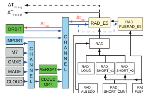
The new submodel RAD now provides a flexible base-model-independent infrastructure for radiation calculation according to the MESSy standard. Figure 1 shows the re-vised structure of RAD and its connection to other sub-models. The right side of the diagram displays the rela-tionship of the Fortran95 modules of the SMCL and the SMIL. In the base-model-independent SMCL the Fortran95 modules RAD_ALBEDO, RAD_LONG and RAD_SHORT (RAD_SHORT_v1 and RAD_SHORT_v2 respectively) are USEd1 by the radiation SMCL module RAD. Two alterna-tive shortwave radiation schemes are possible: the standard ECHAM5 radiation scheme (RAD_SHORT_v1) and the ECHAM5 radiation scheme modified according to Thomas (2008, RAD_SHORT_v2). In RAD_SHORT_v1, simplified assumptions for low aerosol loadings under clear-sky condi-tions are considered. For the sake of efficiency, the effects of multiple reflection and the interactions between aerosol scattering and gaseous absorption were neglected (Thomas, 2008). The assumptions made in RAD_SHORT_v1 are not valid for high aerosol loadings after volcanic eruptions. Thus, in RAD_SHORT_v2 modifications were made in the model to include these effects, showing that multiple re-flection is a dominant effect for particle scattering (for de-tails see Thomas, 2008). Thus, RAD_SHORT_v2 is more accurate. The RAD_SHORT_CMN module contains def-initions and an initialisation subroutine, which are com-monly used in RAD_SHORT_v1 and RAD_SHORT_v2 re-spectively (Fouquart and Bonnel, 1980). If the improved high-resolution shortwave radiation sub-submodel FUBRAD (Nissen et al., 2007; Kunze et al., 2014) is switched on, RAD_FUBRAD is called by RAD_SHORT_CMN from the shortwave calculation RAD_SHORT_v1 or RAD_SHORT_v2. Shortwave radiation fluxes due to ozone and oxygen are then calculated at pressures equal to or lower than 70 hPa in the UV–vis with FUBRAD (replacing the shortwave radiation scheme in RAD). At altitudes above 70 hPa the UV–vis shortwave radiation fluxes are either calcu-lated by RAD_SHORT_v1 in one spectral interval as in the original ECHAM5 code or modified as in RAD_SHORT_v2. A detailed description of the sub-submodel RAD_FUBRAD is presented in Sect. 2.2. In the SMIL the modules RAD_E5 and RAD_FUB_E5 are responsible for the data transfer from the ECHAM5 base model and other submodels to RAD and from RAD via RAD_E5 to the base model. The calculated radiative temperature tendency of the first radiation call pro-vides the temperature feedback (1Tfeed) to the base model
(see Fig. 1). The radiative temperature tendencies from mul-tiple diagnostic calls are also available as diagnostic variables (1Tdiag).
1Fortran95 syntax
Figure 1.Diagram of the revised radiation structure in EMAC. The relationship between the various Fortran95 modules of RAD is given on the right-hand side. The different MESSy layers SMCL and SMIL are indicated. The left-hand side shows the connection of RAD to other submodels. The grey boxes indicate existing submod-els delivering input for the radiation, whereas the green boxes show new submodels, which are now separated from the radiation code. The blue arrows indicate the input to RAD and RAD_FUBRAD (dashed) via the channel infrastructure and the red arrows indicate the trigger, passed from RAD to ORBIT. The black arrows indicate the dependencies of the Fortran95 modules through Fortran USE statements. The direction of the arrows indicates where the differ-ent modules are used. A detailed description is given in the text.
The left side of Fig. 1 shows the connections (mainly for RAD input) via the MESSy infrastructure submodel CHAN-NEL (Jöckel et al., 2010) to other submodels. The RAD input variables are provided by the submodels ORBIT, IMPORT (data import from external files, Kerkweg and Jöckel, 2015), AEROPT, and CLOUDOPT. The input for AEROPT is either provided from the dynamical aerosol models MADE (Lauer et al., 2007), MADE3 (Kaiser et al., 2014), M7 (Vignati et al., 2004), GMXE (Pringle et al., 2010), or from external data via IMPORT. The input for the submodel CLOUDOPT can be selected from the submodel CLOUD or from external data via IMPORT.
The RAD user interface (a specific Fortran95 namelist) allows for a trigger (1trad), which explicitly enables
radia-tion calcularadia-tion, as radiaradia-tion is not obligatorily called every model time step, as it is computationally intensive. The cor-responding time offset is calculated and provided as channel object to the submodel ORBIT. As ORBIT is called every time step, the orbital parameters are calculated with this time offset and are provided as channel objects back to RAD (see Fig. 1).
– A logical switch for the FUBRAD shortwave radiation scheme.
– The specification of the radiation time step. – The possibility to modify the solar constant.
– Logical switches for diagnostically calling the radia-tion scheme multiple times within one model time step. These switches are required for radiative forcing calcu-lations (see details in Sect. 3).
– The choice between the shortwave radiation scheme RAD_SHORT_v1 and RAD_SHORT_v2.
– The selection of 18 input variables (listed in the Sup-plement of this paper), required for the radiation calcu-lation. These input variables are given by channel and channel object selection, for instance, from the channels ORBIT, AEROPT, CLOUDOPT, and IMPORT respec-tively (see Fig. 1). The radiative relevant input variables can either be provided online (via the submodels OR-BIT, AEROPT, CLOUDOPT) or offline (e.g. via IM-PORT in case the variables are available on a geograph-ical grid). For greenhouse gases (GHGs), two other of-fline options are possible besides import of external data fields via IMPORT: the import of constant mixing ratios and of mixing ratios decaying with altitude.
– The FUBRAD namelists are included in the radiation namelist file. Here, the solar cycle conditions and the spectral resolution can be set.
2.2 Sub-submodel RAD_FUBRAD
To achieve a higher spectral resolution for the UV–vis band, the sub-submodel RAD_FUBRAD (Nissen et al., 2007; Kunze et al., 2014) is used. It operates at pressure lev-els above 70 hPa, i.e. in the stratosphere and mesosphere. RAD_FUBRAD substitutes the UV–vis band (250–690 nm) of the RAD shortwave radiation parameterization by either 49 (original version of FUBRAD, Nissen et al., 2007), 55, or alternatively, by 106 bands (Kunze et al., 2014). The scheme is based on the Beer–Lambert law and includes the calcula-tion of shortwave heating rates from the absorpcalcula-tion of UV by O2at the Lyman-αline (121.5 nm, Chabrillat and Kockarts,
1997), the Schumann–Runge continuum and bands (125.5– 205 nm, Strobel, 1978), the calculation of shortwave heat-ing rates from the absorption of UV by O2 and O3 in the
Herzberg continuum (206.2–243.9 nm), and by O3 in the
Hartley (243.9–277.8 nm), Huggins (277.8–362.5 nm), and Chappuis (407.5–690 nm) bands. Efficiency factors accord-ing to Mlynczak and Solomon (1993) are included to ac-count for energy loss due to airglow for the Lyman-αline, the Schumann–Runge continuum, and the Hartley bands. Instead of using Rayleigh scattering in a two stream approximation, backscattering of the atmosphere and surface is considered,
where the albedo atp=70 hPa in the UV–vis (albtsw),
calcu-lated as the ratio of upward↑and downward↓directed flux in the UV–vis (FUV–vis), is used to define the upward directed
flux in the Huggins and Chappuis bands within FUBRAD: albtsw=
FUV–vis↑(p=70 hPa) FUV–vis↓(p=70 hPa)
(1) The coupling to the single UV–vis band, operating at alti-tudes below 70 hPa, is done via a coefficient (FUV–vis_frac),
representing the fraction of downward directed UV–vis flux at 70 hPa to the respective flux at TOA:
FUV–vis_frac=
FUV–vis↓(p=70 hPa) FUV–vis↓(p=0 hPa)
. (2)
When calculating the transmission functions for clear-sky and all-sky conditions at altitudes below 70 hPa,FUV–vis_frac
is the only parameter determined by FUBRAD that is taken into account to attenuate the TOA UV–Vis fluxes. The up-dated version of RAD_FUBRAD has an increased spectral resolution of the Chappuis band (407.5–690 nm) from one band in the original version (Nissen et al., 2007) to either 6 or 57 in the new version (Kunze et al., 2014). The band widths and the corresponding O3absorption cross sections of
the additional Chappuis bands are taken from WMO (1986). With the finer spectral resolution it is now possible to use the observed solar fluxes within each Chappuis band, rather than the original single value, which was scaled to repro-duce the correct heating rate in the original version (Nis-sen et al., 2007). The application of non-scaled fluxes allows to create a consistent UV–vis flux profile of the two com-bined parameterizations over the complete vertical model do-main and consistent flux diagnostics at TOA and the surface. FUBRAD is fully included in RAD with corrected diagnos-tics as shown in Fig. 1. If the sub-submodel FUBRAD is switched on, RAD_FUBRAD is called from the shortwave calculation RAD_SHORT_v1 or RAD_SHORT_v2. In the SMIL the module RAD_FUBRAD_E5 is responsible for the data transfer from the ECHAM5 base model and other sub-models to RAD and from RAD via RAD_E5 to the base model.
The sub-submodel RAD_FUBRAD is controlled by its namelists, featuring the FUBRAD CTRL and CPL namelist, included in the radiation namelist file. Here the spectral res-olution and the solar cycle conditions can be set.
2.3 Submodel AEROPT
The submodel AEROPT carries out the calculation of aerosol optical properties, which are required as input values for the radiation scheme and are provided by coupling the two sub-models via the MESSy CHANNEL infrastructure.
vertically over each grid box), the single scattering albedo (i.e. the ratio of scattering to absorption by the aerosol), and the asymmetry factor (describing the angular distribution of scattering intensity).
Currently there are three options to provide the above men-tioned variables to the radiation scheme.
– The first option is using the aerosol climatology TANRE (Tanre et al., 1984) as in the original radiation code of the ECHAM5 and ECHAM6 models. The TANRE cli-matology provides aerosol concentrations and related aerosol optical properties per unit mass for five differ-ent aerosol types, which can be individually turned on or off. The climatology is implemented in the form of spectral coefficients, which are converted to grid point space during the model initialisation. During runtime, the model calculates relative humidity at each grid cell, which is used in conjunction with the climatological aerosol concentrations from the climatology to calculate the required parameters for the radiation scheme with the help of simplified functions.
– In the second option, the variables can directly be im-ported from a file via the MESSy submodel IMPORT. Therefore, the variables are required on a geographical grid as, for instance, provided by the Chemistry-Climate Model Initiative (CCMI) for stratospheric and volcanic aerosols (see ftp://iacftp.ethz.ch/pub_read/luo/ccmi). – In the third option the optical properties can be
cal-culated online with the help of aerosol tracer concen-trations (component mass and particle number) and their corresponding size distributions. These data can either be provided by external data sources and using passive tracers or calculated online by microphysical aerosol submodels including gas–aerosol partitioning. In the EMAC system there are several aerosol submod-els available such as the modal aerosol modsubmod-els MADE (Lauer et al., 2007), MADE3 (Kaiser et al., 2014), M7 (Vignati et al., 2004), or GMXE (Pringle et al., 2010). The online calculation of the aerosol optical proper-ties is then performed with the help of pre-calculated 3-D lookup tables. The lookup tables provide optical properties of aerosol modes as a function of the real and imaginary part of the refractive index and the Mie size parameter (i.e. aerosol size divided by wavelength, 2π r/λ). The lookup tables are calculated with the radia-tive transfer model code libradtran (Mayer and Kylling, 2005). Libradtran is used to perform the required Mie calculations for a given aerosol population. Here, it is assumed that the aerosol population is log-normally dis-tributed with a given modal width (σ). The radiation scheme then takes the particle number weighted average of the values for extinction cross section, single scatter-ing albedo and asymmetry factor from the lookup ta-ble as input for the radiative transfer calculations.
Dur-ing runtime, a set of lookup tables coverDur-ing all modal widths used within the aerosol submodel is required. For the longwave spectrum only the extinction value is calculated, as the current radiation scheme requires only this parameter.
Aerosol species explicitly considered are water soluble in-organic ions (WASO), black carbon (BC), in-organic carbon (OC), sea salt (SS), mineral dust (DU), and aerosol wa-ter (H2O). The refractive indices for those aerosol species
are extracted from various data sources (most of the data are compiled in the HITRAN2004 database) and include wavelength dependencies. The original references are WASO (mainly using ammonium sulphate values following Hess et al., 1998), BC (Hess et al., 1998), SS (Shettle and Fenn, 1979), H2O (Hale and Query, 1973), OC (Hess et al., 1998;
Sutherland and Khanna, 1991), and DU (Hess et al., 1998). The refractive indices for each aerosol mode required as input for the lookup tables are calculated assuming an inter-nal mixture of the aerosol components for the hydrophilic modes. A mean refractive index is calculated for each mode– wavelength combination by averaging the refractive indices of the individual components weighted with their volume contributions. The corresponding Mie size parameters are de-rived from the median radii of the log-normally distributed modes and the respective wavelengths. The wavelength-dependent particle extinction cross section, single scattering albedo, and asymmetry parameter for each mode are then ob-tained from the lookup table for the appropriate modal width (σ). For the hydrophobic modes the same approach can be selected as well as assuming an external mixture, which re-sults in an averaging of the optical properties of the indi-vidual components. Taking into account the particle number concentrations and the grid box’s vertical extension, the ex-tinction cross sections can be converted into aerosol optical thicknesses. The optical thickness of the whole aerosol pop-ulation in the grid cell is then calculated as the sum over all modes. The mean values of the single scattering albedo and the asymmetry parameter are obtained by averaging over the modes weighted with their optical thickness. To represent mean radiative properties of the aerosol particles for each radiation band, the extinction, single scattering albedo, and the asymmetry factor are determined for fixed representative wavelength values and then mapped onto the corresponding radiation bands using a weighting with the solar spectrum.
This technique of calculating the aerosol optical properties online from the simulated aerosol concentrations and lookup tables has been applied earlier by Lauer et al. (2007), Pozzer et al. (2012), Pozzer et al. (2015), de Meij et al. (2012), Tost and Pringle (2012), and Righi et al. (2013, 2015).
are required for the radiation calculation are provided via the MESSy CHANNEL interface. Consequently, the coupling structure of the respective radiation call can be provided with the information of aerosol optical properties, which are sup-posed to be used for the respective radiative transfer calcula-tions. Note that multiple diagnostic calls of the radiation with different aerosol settings are possible.
As mentioned before, AEROPT is equipped with the op-tion to collect data from external sources, e.g. imported from files via IMPORT, or from alternative aerosol schemes, which provide their own calculation of the respective val-ues required for aerosol–radiation interactions. In addition, AEROPT can provide the aerosol optical properties required for the calculation of photolysis rates, as e.g. used by the submodel JVAL (Sander et al., 2014). For this purpose scat-tering, absorption, and asymmetry factor can be calculated at additional wavelengths required by JVAL and provided as channel objects.
Besides the three options of providing optical properties to AEROPT, it is also possible to merge two different datasets for aerosol optical properties in the vertical, e.g. using prog-nostic tropospheric aerosol values combined with the values provided by CCMI for the stratospheric aerosol for the radia-tion calcularadia-tions. The merging of two datasets can be done at a given height or as a linear interpolation in pressure between two reference values. It is also possible to add two datasets, for instance in the case of missing volcanic aerosols, the cor-responding aerosol optical properties can be provided by an external data source and combined with the online calculated values for prognostic aerosols. The user settings are con-trolled via namelists (a detailed description of the namelist settings of AEROPT can be found in the Supplement of this paper):
– the information (a counting index and the corresponding filenames of the lookup tables) about the desired lookup tables used (shortwave and longwave spectrum are han-dled separately);
– the information about the sets of aerosol radiative prop-erties (e.g. GMXE, M7, MADE, MADE3, TANRE), which explain how the optical properties are going to be calculated (mixing rules, exclusion for certain species, coupling to required input parameters, etc.);
– the option to read a set of aerosol radiative properties from external sources;
– the feature to merge two different datasets of aerosol radiative properties, as required for the RAD submodel, which can either be read in via the external interface or be calculated by AEROPT (or an alternative submodel for calculating aerosol optical properties). Additionally, optional weighting factors can be included.
2.4 Submodel CLOUDOPT
The optical properties of clouds are now calculated in the EMAC submodel CLOUDOPT. The input variables needed for calculating cloud optical properties are cloud cover, cloud liquid and cloud ice water, and cloud nuclei concentration. These optical properties are diagnosed at each band to ac-count for their wavelength dependency. The specific relations for the solar spectral bands are based on Mie calculations as given by Rockel et al. (1991). A specific correction for the asymmetry factor is applied to account for the non-sphericity of ice crystals (Roeckner et al., 2003). Coefficients for the single scattering albedo, the asymmetry factor, and the mass extinction are given for cloud liquid droplets and ice crystals. These coefficients are provided for four bands of the short-wave spectrum and for 16 bands of the longshort-wave spectrum. Mass absorption coefficients for liquid and ice clouds are pa-rameterized as described by Roeckner et al. (2003) based on classical approaches from Stephens et al. (1990) and Ebert and Curry (1992). Calculated cloud optical properties then serve as input for the radiation calculation comprising the shortwave and longwave optical depth, the asymmetry fac-tor, and the single scattering albedo of cloud particles. For the 2-D or total cover in the radiation computation of EMAC the default cloud overlap assumption is maximum-random overlap; maximum overlap and random overlap are also pos-sible.
The CLOUDOPT namelists (see detailed description in the Supplement of this paper) comprise mainly four items.
– The model resolution-dependent parameters are set, such as a correction factor for the asymmetry factor of ice clouds, the cloud inhomogeneity factors of ice and liquid water, and a parameter to correct the asymmetry factor of ice clouds. The corresponding (hard-wired) de-fault values of these parameters can thus be overwritten without re-compilation of the code.
– The channel and channel object names of the required input fields are specified: cloud cover, cloud liquid wa-ter, cloud ice, and cloud nuclei concentration.
– The effective radii of liquid droplets and/or ice can be calculated internally or provided by an external channel object.
– The number of (diagnostic) calls of CLOUDOPT in each model time step is selected. The required input is set individually for each call.
for example the evaluation of the performance of the radia-tion code with respect to a benchmark test, similar to Myhre et al. (2009, see the example benchmark test in Sect. 3.4). 2.5 Submodel ORBIT
In the new infrastructure of the EMAC radiation calculation the orbital parameters are separated from the radiation cal-culation. They are now calculated in the submodel ORBIT. Orbital parameters are depending on the time of the day and the year. The basic equations used are the Kepler equation for the eccentric anomaly and Lacaille’s formula (see Roeckner et al., 2006).
The radiation submodel RAD now accesses the necessary channel objects of the orbital parameters, including the dis-tance of the sun to the earth, the cosines of the zenith angle, and the relative day length. As the radiation is not calculated every time step, ORBIT also receives information from RAD (see Fig. 1), namely the offset for the radiation calculation (1trad).
The ORBIT namelists (see detailed description of these namelists in the Supplement of the paper) comprise
– the selection/setting of the orbital parameters, such as the eccentric anomaly, the inclination, and the longitude of perihelion;
– the possibility to distinguish between two orbit calcula-tions, for either annual cycle or perpetual month exper-iments respectively;
– the channel object containing the radiation calculation offset1trad.
2.6 Example application: volcanic heating rates To demonstrate the functionality of the new radiation infras-tructure, we show a test case: the eruption of Mt. Pinatubo in June 1991, which injected SO2into the stratosphere and
thus modified the radiative balance by additional radiative heating. For our simulations with the revised EMAC radia-tion infrastructure, we chose a 90-layer model setup (up to 0.01 hPa, approx. 80 km) with a spectral truncation T42 of the dynamical ECHAM5 core. Interactive chemistry was not simulated, but AEROPT was used to provide two different sets of aerosol optical properties: (1) the standard TANRE climatology (i.e. without additional volcanic aerosol) and (2) the standard TANRE climatology combined (MERGED) with the offline stratospheric aerosol data as provided by CCMI. Note that the gas phase of SO2is not radiatively
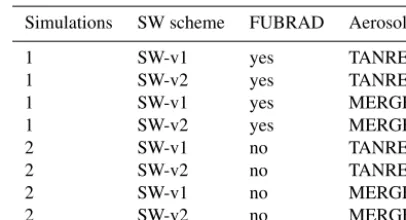
ac-tive in our model. In one model simulation, the RAD calcu-lation was performed four times every third model time step: each aerosol input (TANRE or MERGED) combined with each shortwave radiation scheme (SW-v1 or SW-v2). The simulation has been performed twice, without and with the FUBRAD scheme respectively. The resulting eight different radiation setups are summarized in Table 1.
Table 1.Radiation setups (modified heating rates due to the erup-tion of Mt. Pinatubo) used for testing the new radiaerup-tion infrastruc-ture. Both simulations cover the years 1991–1993. Varied parame-ters are the shortwave scheme (SW-v1 or SW-v2), the selection of the FUBRAD radiation scheme, and the selected aerosol input to AEROPT (TANRE or MERGED).
Simulations SW scheme FUBRAD Aerosol
1 SW-v1 yes TANRE
1 SW-v2 yes TANRE
1 SW-v1 yes MERGED
1 SW-v2 yes MERGED
2 SW-v1 no TANRE
2 SW-v2 no TANRE
2 SW-v1 no MERGED
2 SW-v2 no MERGED
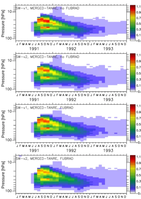
Figure 2 shows the resulting simulated volcanic heating rates (in K day−1) for the years 1991 to 1993 from the erup-tion of Mt. Pinatubo. The volcanic heating rates are given as difference between the heating rates simulated with volcanic aerosol (MERGED) and the heating rate simulated without volcanic aerosol (TANRE). The values are averaged for the tropics, i.e. over 5◦N–5◦S. The comparison of our model re-sults with the study of Stenchikov et al. (1998) shows that in August 1991 and January 1992 the zonally averaged heat-ing rates (pictures are not shown) are structurally in good agreement: in August 1991 the maximum is between 0 and 10◦S at 20 hPa but up to 0.9 K day−1 larger in our model setup. Also, January 1992 shows structurally good agreement with the study of Stenchikov et al. (1998). As expected, the patterns in Fig. 2 are similar for the different setups, since the aerosol optical properties are prescribed. Nevertheless, in the pattern for the different setups differences with respect to the absolute values occur. The maximum heating rates are larger for the SW-v1 scheme compared to the SW-v2 scheme. Shortwave heating rates are overestimated by SW-v1 as a result of the simplified assumptions for low aerosol load-ings under clear-sky conditions; these assumptions are not valid for high aerosol loadings after volcanic eruptions. The heating rates from SW-v2 are more accurate, as the effects of multiple reflection and the interactions between aerosol scattering and gaseous absorption (which are important for high aerosol loadings after volcanic eruptions) are consid-ered here, in contrast to SW-v1 (Thomas, 2008).
Pressure [hPa]
Pressure [hPa]
Pressure [hPa]
Pressure [hPa]
Figure 2.Simulated temporal evolution versus pressure altitude of
the volcanic heating rates (in K day−1) in the tropics (5◦S–5◦N)
due to the eruption of Mt. Pinatubo in June 1991. The different pan-els show the results for SW-v1 and SW-v2 of the shortwave scheme, both with and without FUBRAD (as indicated).
3 Calculation of radiative forcing
3.1 Technical implementation of radiative forcing calculation in RAD
A new feature in the radiation submodel RAD is the user-friendly and flexible implementation of the online radiative forcing calculation. It is now possible to determine instanta-neous as well as stratosphere-adjusted radiative forcing on-line, i.e. during the model simulation, by multiple calls of the radiation scheme. Instantaneous radiative forcing is de-fined as the change in the net radiative flux with atmospheric temperatures held fixed to unperturbed values. In contrast, the concept of stratosphere-adjusted radiative forcing, also known as the fixed dynamic heating concept (Ramanathan and Dickinson, 1979; Fels et al., 1980), allows stratospheric temperatures to adjust to a new radiative equilibrium, with-out changes in tropospheric variables and stratospheric dy-namics. Since the first IPCC report (Houghton et al., 1990), stratosphere-adjusted radiative forcing has been the preferred
metric used to quantify and rank the numerous components impacting the global climate.
The technical procedure to determine the stratosphere-adjusted radiative forcing within a climate model simula-tion was introduced by Stuber et al. (2001) to the climate model ECHAM4. A second diagnostic temperature field is implemented to calculate the stratosphere-adjusted radiative forcing. The reference atmosphere controlled by the first ra-diation call is not subject to the perturbations; however, the temperature field of the extra diagnostic radiation call experi-ences additional radiative heating above the tropopause, with dynamical heating remaining identical to the unperturbed reference atmosphere. In the troposphere, the reference tem-perature and the perturbated diagnostic temtem-perature are iden-tical. To enable the stratospheric temperature to readjust to the new equilibrium, a spin-up period of at least 3 months must be considered (Manabe and Strickler, 1964).
After improving the radiation code structure (see Sect. 2.1), multiple diagnostic calls of the radiation routine can easily be made in order to determine radiative forcing. Via namelist selection (for detailed description of the ra-diation namelist see Supplement) rara-diation routines can be called several times within one simulation. The first call is always the reference call and provides the temperature feed-back 1Tfeed (see Fig. 1), the other calls are of diagnostic
nature. Either instantaneous or stratosphere-adjusted radia-tive forcing can be selected by a namelist switch. With this setup the radiative forcing of various GHG, aerosol, or cloud perturbations can be calculated simultaneously in one model simulation. GHG perturbations can be given as constant mix-ing ratios with or without vertical gradient, as externally pre-scribed 3-D distributions, or as online calculated, 3-D fields. All perturbed values are specified via channel object selec-tion in the radiaselec-tion namelist (see detailed descripselec-tion in the Supplement). Hence, radiative forcing can be calculated without extra simulation.
Table 2.Annually and globally averaged shortwave (SW), longwave (LW), and net instantaneous and stratosphere-adjusted radiative forcing
at the tropopause due to changes in CO2and stratospheric O3between 1980 and 2000 and due to additional homogeneous 1 % contrail cover.
The respective values of the radiative forcing at TOA are given in parentheses.
Instantaneous RF Adjusted RF
CO2 Strat. O3 Contrail CO2 Strat. O3 Contrail
SW 0.002 (0.05) 0.08 (−0.13) −0.088 (−0.086) 0.002 (0.05) 0.08 (−0.14) −0.088 (−0.086)
LW 0.48 (0.23) −0.02 (−0.03) 0.203 (0.195) 0.45 (0.40) −0.09 (0.13) 0.201 (0.199)
Net 0.48 (0.27) 0.06 (−0.16) 0.115 (0.109) 0.45 (0.45) −0.01 (−0.01) 0.113 (0.113)
3.2 Example 1: radiative forcing of CO2increase
The concept of stratosphere-adjusted radiative forcing is well known and well established for the case of CO2change. Its
features and merits are repeated here mainly to set the scene for the more interesting non-CO2cases. The first example,
thus, forms a radiative forcing calculation with EMAC us-ing a CO2increase of 28.8 ppmv, representing the change of
CO2in 2000 relative to 1980. This CO2change was
calcu-lated by the EMAC hind-cast simulation RC1-base-08. The model setup of this simulation is described in detail by Jöckel et al. (2016). Table 2 lists global mean values for the instan-taneous and stratosphere-adjusted radiative forcing, both at TOA (given in brackets) and at the annual mean tropopause, while Fig. 3 illustrates the vertical structure of the longwave, shortwave, and net radiative flux changes induced by the CO2
increase.
The main radiative impact of CO2occurs in the longwave
part of the spectrum, whereas the shortwave forcing com-ponent is almost zero at the tropopause (but about 18 % of the net at TOA because of NIR absorption in the middle at-mosphere). The stratosphere-adjusted net radiative forcing (0.45 W m−2) is about 7 % smaller than the instantaneous net radiative forcing at the tropopause, qualitatively confirm-ing previous findconfirm-ings. The reason for the dampenconfirm-ing, when stratospheric adjustment is included, is the cooling effect of additional CO2 in the stratosphere, reducing the downward
longwave flux into the troposphere. The instantaneous net radiative forcing is considerably smaller at TOA compared to the tropopause for the CO2 case (0.27 and 0.48 W m−2
respectively). The effect of stratospheric temperature adjust-ment is to create a new balance of shortwave and long-wave fluxes, leading to vertically constant net radiative flux changes above the tropopause (Fig. 3, bottom). Hence, the stratosphere-adjusted net radiative forcing has the same value at TOA and at the tropopause. Note, however, that this does not hold for the shortwave and longwave components.
Model dependencies in radiative forcing may arise not only from the specific radiative transfer scheme used in a given model (here: EMAC) but also from methodical aspects as discussed by e.g. Forster et al. (1997). In particular, as mentioned above, in our showcases a fixed tropopause from an EMAC reference simulation is used to define the domain
−0.1 0 0.1 0.2 0.3 0.4 0.5 0.6
Top
0.03
0.1
0.3
1
3
10
30
100
300
1000
Instant. Radiative Forcing (EMAC, global 2000−1980 CO2)
Radiative flux [W/m**2]
Altitude [hPa]
SW forcing LW forcing Net forcing
−0.1 0 0.1 0.2 0.3 0.4 0.5 0.6
Top
0.03
0.1
0.3
1
3
10
30
100
300
1000
Adjusted Radiative Forcing (EMAC, global 2000−1980 CO2)
Radiative flux [W m ]
Altitude [hPa]
-2
Figure 3.Vertical profile of the global and annual mean net, short-wave, and longwave instantaneous radiative flux change (top) and of
the stratosphere-adjusted radiative flux change (bottom) in W m−2,
resulting from CO2change between 1980 and 2000.
Pressure/hP
a
º S º S º N º N
Figure 4.Zonal geographical distribution of the annual mean
strato-spheric O3change between 1980 and 2000.
calculations. A consequence is that the stratosphere-adjusted radiative forcing profile above the tropopause is constant only in the annual mean. However, as already discussed by Forster et al. (1997), this must not be viewed as a concep-tual disadvantage, and the online radiative forcing calcula-tions in a chemistry–climate model (CCM)like EMAC may have dedicated advantages for many non-CO2forcings (see
Sect. 3.3).
3.3 Example 2: radiative forcing of an ozone-hole like perturbation
The challenge to provide a meaningful indicator of the ex-pected climate effect of ozone concentration perturbations led to establishing stratosphere-adjusted radiative forcing as a standard procedure for a long time. This example uses a stratospheric ozone change due to stratospheric ozone destruction evolving between 1980 and 2000, again from the EMAC hind-cast simulation RC1-base-08 (see above). The respective stratospheric ozone change pattern, shown in Fig. 4 as an annual mean, is in good agreement with obser-vations (see Hassler et al., 2013, their Fig. 8). However, the seasonal cycle is included in the radiative forcing calcula-tions.
In agreement with previous experience (Ramanathan and Dickinson, 1979; Hansen et al., 1997; Forster and Shine, 1997; Christiansen, 1999) the instantaneous net radiative forcing turns out to be extremely ambiguous for this kind of stratospheric ozone perturbation. It changes sign (see Table 2) from TOA (−0.16 W m−2) to the tropopause (+0.06 W m−2), a feature controlled by the shortwave com-ponent: less ozone absorption above the tropopause means an energy gain for the troposphere/surface system but an en-ergy loss for the whole atmosphere. Less shortwave
absorp-tion above the troposphere, as occurring in this case, means a cooling and changes the downward longwave radiative flux at the tropopause to an extent that the net radiative forcing at the tropopause changes sign (Fig. 5), giving a small negative value of−0.01 W m−2for the stratosphere-adjusted radiative forcing. As pointed out by Hansen et al. (1997) the negative net forcing has the correct sign to predict a cooling effect in the troposphere/surface system as a result of ozone deple-tion. Quantitatively our value is smaller than the respective estimate given in the last two IPCC reports (−0.05 W m−2), which are based on ozone loss over the period where ozone depleting substances have increased. However, our value is close to the estimate of−0.02 W m−2 provided within the ACCMIP project (Myhre et al., 2013, their Table 8.3), where simulated ozone changes induced by various effects were used for the calculation. In the present paper our key point is to underpin the usefulness of having a method at hand, which allows to calculate the stratosphere-adjusted forcing at the tropopause online in a CCM.
3.4 Example 3: cloud perturbations
The necessity to calculate radiative forcings for cloud changes may arise in context of direct anthropogenic cloud cover change as induced by contrails or ship tracks. It is more realistic to perform such calculations on a time step ba-sis within a CCM rather than using monthly mean input for an offline radiative transfer model. For example, Frömming et al. (2011) found a reduction of contrail radiative forcing of about 20 % when time-varying (instead of time-averaged) contrail optical depth is used. Rap et al. (2010) even report a reduction of all-sky contrail radiative forcing of more than 35 % when daily correlation of contrails and natural clouds is accounted for rather than using time mean cloud and contrail properties.
−0.2 −0.15 −0.1 −0.05 0 0.05 0.1 0.15 Top
0.03
0.1
0.3
1
3
10
30
100
300
1000
Radiative flux [W/m**2]
Altitude [hPa]
SW forcing LW forcing Net forcing
−0.2 −0.15 −0.1 −0.05 0 0.05 0.1 0.15 Top
0.03
0.1
0.3
1
3
10
30
100
300
1000
Adjusted Radiative Forcing (EMAC, global 2000−1980 strat−O3)
Radiative flux [W m ]
Altitude [hPa]
-2
Figure 5.Vertical profile of the global and annual mean net, short-wave, and longwave instantaneous radiative flux change (top) and of
the stratosphere-adjusted radiative flux change (bottom) in W m−2,
resulting from stratospheric O3change between 1980 and 2000.
at TOA, we determine the net radiative forcing at the mean tropopause, which is 0.115 W m−2. Furthermore, we calcu-lated the stratosphere-adjusted radiative forcing, which was found to be 0.113 W m−2(net), deviating only by 4 % from the instantaneous radiative forcing at TOA.
Figure 6 shows the geographical distribution of the annual mean net radiative forcing at TOA for 1 % homogeneous con-trail cover. The spatial pattern is dominated by the distribu-tion of natural clouds. The net radiative forcing of the added contrails is high where natural cloud cover is low, e.g. over deserts, and is comparatively low in regions with high natu-ral cloud cover, e.g. over the tropics and mid-latitudes. The magnitude of the minima and maxima, as well as the spatial pattern of the net radiative forcing, looks similar to the re-sults presented in the intercomparison study of Myhre et al. (2009). Despite its conceptual advantages over offline radia-tive transfer models, this benchmark test confirms the
suit-90 N0
60 N0
30 N0
00
30 S0
60 S0
90 S0
[W m ]-2
180 150 W 120 W 90 W 60 W 30 W 0 30 E 60 E 90 E 120 E 150 E 1800 0 0 0 0 0 0 0 0 0 0 0 0
Figure 6.Geographical distribution of the annual mean net instan-taneous radiative forcing at TOA for a homogeneous 1 % contrail cover.
ability of the submodel RAD with respect to calculating the radiative effects of thin ice clouds and contrails.
4 Summary
The submodel RAD (including the shortwave radiation scheme RAD_FUBRAD) provides a flexible and base-model-independent infrastructure of the radiation transfer calculation according to the MESSy standard. With the new submodels AEROPT, CLOUDOPT, and ORBIT the calcula-tions of aerosol and cloud optical properties, as well as the calculation of orbital parameters, are now performed within these independent submodels, after having them outsourced from the previous radiation code RAD4ALL. All these new submodels are coupled via the standard MESSy infrastruc-ture to RAD (see Fig. 1).
In the new radiation infrastructure online or offline vari-ables, which are needed for the radiation calculation, are se-lected via namelists. Offline input as e.g. climatologies of radiatively active gases, are now read via the submodel IM-PORT, instead of importing them within the radiation code. Thus, the submodel RAD can be applied to easily define dif-ferent radiation setups with almost arbitrary inputs. Multiple diagnostic calls of the radiation routine are possible in RAD and, as by-product, radiative forcing can be calculated during the model simulation.
In the present paper example applications of the now im-plemented radiative forcing calculations show the wide spec-trum of possible radiative forcing calculations within EMAC.
5 Code and data availability
In-stitutions can be a member of the MESSy Consortium by signing the MESSy Memorandum of Understanding. More information can be found on the MESSy Consortium web-site (http://www.messy-interface.org). All modifications and new diagnostics presented in this paper are implemented in the MESSy versions 2.51 and 2.52.
The Supplement related to this article is available online at doi:10.5194/gmd-9-2209-2016-supplement.
Acknowledgements. We thank Tobias Zinner for providing the radiative transfer model libradtran, which was used to prepare the lookup tables of the Mie size parameters. This work was partly supported by the German Research Foundation (DFG) Research Unit 1095 “Stratospheric Change and its Role for Climate Prediction” (SHARP) and the DLR-project “Verkehrsentwicklung und Umwelt” (VEU). The model simulation RC1-base-08 used for radiative forcing calculations has been performed at the German Climate Computing Centre DKRZ through support from the Bundesministerium für Bildung und Forschung (BMBF).
The article processing charges for this open-access publication were covered by a Research
Centre of the Helmholtz Association.
Edited by: O. Morgenstern
References
Chabrillat, S. and Kockarts, G.: Simple parameterization of the
ab-sorption of the solar Lyman-α line, Geophys. Res. Lett., 24,
2659–2662, 1997.
Christiansen, B.: Radiative forcing and climate sensitivity: The ozone experience, Q. J. Roy. Meteor. Soc., 125, 3011–3035, 1999.
Chung, E.-S. and Soden, B.: An Assessment of Direct Radiative Forcing, Radiative Adjustments, and Radiative Feedbacks in Coupled Ocean Atmosphere Models, J. Climate, 28, 4152–4170, doi:10.1175/JCLI-D-14-00436.1, 2015.
de Meij, A., Pozzer, A., Pringle, K. J., Tost, H., and Lelieveld, J.: EMAC model evaluation and analysis of at-mospheric aerosol properties and distribution with a focus on the Mediterranean region, Atmos. Res., 114-115, 38–69, doi:10.1016/j.atmosres.2012.05.014, 2012.
Ebert, E. and Curry, J.: A parameterization of cirrus cloud optical properties for climate models, J. Geophys. Res., 97, 3831–3836, 1992.
Fels, S., Mahlman, J., Schwarzkopf, M., and Sinclair, R.: Strato-spheric sensitivity to perturbations in ozone and carbon diox-ide: radiative dynamical response, J. Atmos. Sci., 37, 2265–2297, 1980.
Forster, P., Freckleton, R., and Shine, K.: On aspects of the concept of radiative forcing, Clim. Dynam., 13, 547–560, 1997.
Forster, P. d. F. and Shine, K.: Radiative forcing and temperature trends from stratospheric ozone changes, J. Geophys. Res., 102, 10841–10855, 1997.
Forster, P. M., Fomichev, V. I., Rozanov, E., Cagnazzo, C., Jon-sson, A. I., Langematz, U., Fomin, B., Iacono, M. J., Mayer, B., Mlawer, E., Myhre, G., Portmann, R. W., Akiyoshi, H., Falaleeva, V., Gillett, N., Karpechko, A., Li, J., Lemennais, P., Morgenstern, O., Oberländer, S., Sigmond, M., and Shibata, K.: Evaluation of radiation scheme performance within chem-istry climate models, J. Geophys. Res.-Atmos., 116, D10302, doi:10.1029/2010JD015361, 2011.
Fouquart, Y. and Bonnel, B.: Computations of solar heating of the Earth’s atmosphere: A new parameterization, Beitr. Phys. At-mos., 53, 35–62, 1980.
Frömming, C., Ponater, M., Burkhardt, U., Stenke, A., Pechtl, S., and Sausen, R.: Sensitivity of contrail coverage and contrail ra-diative forcing to selected key parameters, Atmos. Environ., 45, 1483–1490, doi:10.1016/j.atmosenv.2010.11.033, 2011. Hale, G. and Query, M.: Optical constants of water in the 200 nm to
200 µ wavelength region, Appl. Optics, 12, 555–563, 1973. Hansen, J., Sato, M., and Ruedy, R.: Radiative forcing and climate
response, J. Geophys. Res., 102, 6831–6864, 1997.
Hassler, B., Young, P. J., Portmann, R. W., Bodeker, G. E., Daniel, J. S., Rosenlof, K. H., and Solomon, S.: Comparison of three ver-tically resolved ozone data sets: climatology, trends and radiative forcings, Atmos. Chem. Phys., 13, 5533–5550, doi:10.5194/acp-13-5533-2013, 2013.
Hess, M., Koepke, P., and Schult, I.: Optical Properties of Aerosols and Clouds: The software package OPAC, B. Am. Meteorol. Soc., 79, 831–844, 1998.
Houghton, J., Jenkins, G., and Ephraums, J.: Climate Change: The IPPC Scientific Assessment, Cambridge University Press, Cam-bridge, UK, 1990.
Jöckel, P.: Technical note: Recursive rediscretisation of geo-scientific data in the Modular Earth Submodel System (MESSy), Atmos. Chem. Phys., 6, 3557–3562, doi:10.5194/acp-6-3557-2006, 2006.
Jöckel, P., Sander, R., Kerkweg, A., Tost, H., and Lelieveld, J.: Tech-nical Note: The Modular Earth Submodel System (MESSy) – a new approach towards Earth System Modeling, Atmos. Chem. Phys., 5, 433–444, doi:10.5194/acp-5-433-2005, 2005.
Jöckel, P., Tost, H., Pozzer, A., Brühl, C., Buchholz, J., Ganzeveld, L., Hoor, P., Kerkweg, A., Lawrence, M. G., Sander, R., Steil, B., Stiller, G., Tanarhte, M., Taraborrelli, D., van Aardenne, J., and Lelieveld, J.: The atmospheric chemistry general circulation model ECHAM5/MESSy1: consistent simulation of ozone from the surface to the mesosphere, Atmos. Chem. Phys., 6, 5067– 5104, doi:10.5194/acp-6-5067-2006, 2006.
Jöckel, P., Kerkweg, A., Pozzer, A., Sander, R., Tost, H., Riede, H., Baumgaertner, A., Gromov, S., and Kern, B.: Development cycle 2 of the Modular Earth Submodel System (MESSy2), Geosci. Model Dev., 3, 717–752, doi:10.5194/gmd-3-717-2010, 2010. Jöckel, P., Tost, H., Pozzer, A., Kunze, M., Kirner, O.,
Submodel System (MESSy) version 2.51, Geosci. Model Dev., 9, 1153–1200, doi:10.5194/gmd-9-1153-2016, 2016.
Kaiser, J. C., Hendricks, J., Righi, M., Riemer, N., Zaveri, R. A., Metzger, S., and Aquila, V.: The MESSy aerosol sub-model MADE3 (v2.0b): description and a box sub-model test, Geosci. Model Dev., 7, 1137–1157, doi:10.5194/gmd-7-1137-2014, 2014.
Kerkweg, A. and Jöckel, P.: The infrastructure MESSy submodels GRID (v1.0) and IMPORT (v1.0), Geosci. Model Dev. Discuss., 8, 8607–8633, doi:10.5194/gmdd-8-8607-2015, 2015.
Kunze, M., Godolt, M., Langematz, U., Grenfell, J., Hamann-Reinus, A., and Rauer, H.: Investigating the early Earth faint young Sun problem with a general circulation model, Planet. Space Sci., 98, 77–92, doi:10.1016/j.pss.2013.09.011, 2014. Lauer, A., Eyring, V., Hendricks, J., Jöckel, P., and Lohmann, U.:
Global model simulations of the impact of ocean-going ships on aerosols, clouds, and the radiation budget, Atmos. Chem. Phys., 7, 5061–5079, doi:10.5194/acp-7-5061-2007, 2007.
Manabe, S. and Strickler, R.: Thermal equilibrium of the atmo-sphere with convective adjustment, J. Atmos. Sci., 21, 361–385, 1964.
Mayer, B. and Kylling, A.: Technical note: The libRadtran soft-ware package for radiative transfer calculations – description and examples of use, Atmos. Chem. Phys., 5, 1855–1877, doi:10.5194/acp-5-1855-2005, 2005.
Mlawer, E. J., Taubman, S. J., Brown, P. D., Iacono, M. J., and Clough, S. A.: Radiative transfer for inhomogeneous atmo-spheres: RRTM, a validated correlated-k model for the longwave, J. Geophys. Res., 102, 16663–16682, 1997.
Mlynczak, M. G. and Solomon, S.: A detailed evaluation of the heating efficiency in the middle atmosphere, J. Geophys. Res.-Atmos., 98, 10517–10541, doi:10.1029/93JD00315, 1993. Myhre, G., Kvalevag, M., Raedel, G., Cook, J., Shine, K., Clark, H.,
Karcher, F., Markowicz, K., Kardas, A., Wolkenberg, P., Balkan-ski, Y., Ponater, M., Forster, P., Rap, A., and Rodriguez de Leon, R.: Intercomparison of radiative forcing calculations of strato-spheric water vapour and contrails, Meteorol. Z., 18, 585–596, doi:10.1127/0941-2948/2009/0411, 2009.
Myhre, G., Shindell, D., Breon, F.-M., Collins, W., Fuglestvedt, J., Huang, J., Koch, D., Lamarque, J.-F., Lee, D., Mendoza, B., Nakajima, T., Robock, A., Stephens, G., Takemura, T., and Zhang, H.: Anthropogenic and Natural Radiative Forcing, edited by: Stocker, T. F., Qin, D., Plattner, G.-K., Tignor, M. M. B., Allen, S. K., Boschung, J., Nauels, A., Xia, Y., Bex, V., and Midgley, B.M., Climate Change 2013: The Physical Science Ba-sis, Tech. rep., 2013.
Nissen, K. M., Matthes, K., Langematz, U., and Mayer, B.: Towards a better representation of the solar cycle in general circulation models, Atmos. Chem. Phys., 7, 5391–5400, doi:10.5194/acp-7-5391-2007, 2007.
Pozzer, A., de Meij, A., Pringle, K. J., Tost, H., Doering, U. M., van Aardenne, J., and Lelieveld, J.: Distributions and regional bud-gets of aerosols and their precursors simulated with the EMAC chemistry-climate model, Atmos. Chem. Phys., 12, 961–987, doi:10.5194/acp-12-961-2012, 2012.
Pozzer, A., de Meij, A., Yoon, J., Tost, H., Georgoulias, A. K., and Astitha, M.: AOD trends during 2001–2010 from observations and model simulations, Atmos. Chem. Phys., 15, 5521–5535, doi:10.5194/acp-15-5521-2015, 2015.
Pringle, K. J., Tost, H., Message, S., Steil, B., Giannadaki, D., Nenes, A., Fountoukis, C., Stier, P., Vignati, E., and Lelieveld, J.: Description and evaluation of GMXe: a new aerosol submodel for global simulations (v1), Geosci. Model Dev., 3, 391–412, doi:10.5194/gmd-3-391-2010, 2010.
Ramanathan, V. and Dickinson, R.: The role of stratospheric ozone in the zonal and seasonal radiative energy balance of the Earth-troposphere system, J. Atmos. Sci., 36, 1084–1104, 1979. Rap, A., Forster, P., Jones, A., Boucher, O., Haywood, J.,
Bel-louin, N., and De Leon, R.: Parameterisation of contrails in the UK Met Office Climate Model, J. Geophys. Res, 115, D10205, doi:10.1029/2009JD012443, 2010.
Righi, M., Hendricks, J., and Sausen, R.: The global impact of the transport sectors on atmospheric aerosol: simulations for year 2000 emissions, Atmos. Chem. Phys., 13, 9939–9970, doi:10.5194/acp-13-9939-2013, 2013.
Righi, M., Eyring, V., Gottschaldt, K.-D., Klinger, C., Frank, F., Jöckel, P., and Cionni, I.: Quantitative evaluation of ozone and selected climate parameters in a set of EMAC simulations, Geosci. Model Dev., 8, 733–768, doi:10.5194/gmd-8-733-2015, 2015.
Rockel, B., Raschke, E., and Weyres, B.: A parameterization of broad band radiative transfer properties of water, ice and mixed clouds, Beitr. Phys. Atmosph., 64, 1–12, 1991.
Roeckner, E., Bäml, G., Bonaventura, L., Brokopf, R., Esch, M., Giorgetta, M., Hagemann, S., Kirchner, I., Kornblueh, L., Manzini, E., Rhodin, A., Schlese, U., Schulzweida, U., and Tompkins, A.: The atmospheric general circulation model ECHAM5. Part I: Model description., Max Planck Institute for Meteorology Rep. 249, 127 pp., 2003.
Roeckner, E., Brokopf, R., Esch, M., Giorgetta, M., Hagemann, S., Kornblueh, L., Manzini, E., Schlese, U., and Schulzweida, U.: Sensitivity of simulated climate to horizontal and vertical reso-lution in the ECHAM5 atmosphere model, J. Climate, 19, 3771– 3791, 2006.
Sander, R., Jöckel, P., Kirner, O., Kunert, A. T., Landgraf, J., and Pozzer, A.: The photolysis module JVAL-14, compatible with the MESSy standard, and the JVal PreProcessor (JVPP), Geosci. Model Dev., 7, 2653–2662, doi:10.5194/gmd-7-2653-2014, 2014.
Shettle, E. and Fenn, R.: Models for the aerosols of the lower at-mosphere and the effects of humidity variations on their optical properties, Rep. AFGL-TR-79-0214, Air Force Geophysics Lab., 1979.
Stenchikov, G. L., Kirchner, I., Robock, A., Graf, H.-F., Antuña, J. C., Grainger, R. G., Lambert, A., and Thomason, L.: Radiative forcing from the 1991 Mount Pinatubo volcanic eruption, J. Geo-phys. Res.-Atmos., 103, 13837–13857, doi:10.1029/98JD00693, 1998.
Stephens, G., Tsay, S.-C., Stackhouse, P., and Flateau, P.: The rel-evance of the microphysical and radiative properties of cirrus clouds to climate and climate feedback, J. Atmos. Sci., 47, 1742– 1753, 1990.
Strobel, D. F.: Parameterization of the atmospheric heating rate
from 15 to 120 km due to O2and O3absorption of solar
radi-ation, J. Geophys. Res., 83, 6225–6230, 1978.
Sutherland, R. and Khanna, R.: Optical Properties of Organic-based Aerosols Produced by Burning Vegetation, Aerosol Sci. Tech., 14, 3, 331–342, doi:10.1080/02786829108959495, 1991. Tanre, D., Geleyn, J.-F., and Slingo, J.: First results of the
introduc-tion of an advanced aerosol-radiaintroduc-tion interacintroduc-tion in the ecmwf low resolution global model, in: Aerosols and their Climatic Ef-fects, edited by: Gerber, H. and Deepak, A., 133–177, 1984. Thomas, M.: Simulation of the climate impact of Mt. Pinatubo
erup-tion using ECHAM5, Reports on Earth System Science 52, Max Planck Institute for Meteorology, Hamburg, 2008.
Tost, H. and Pringle, K. J.: Improvements of organic aerosol rep-resentations and their effects in large-scale atmospheric models, Atmos. Chem. Phys., 12, 8687–8709, doi:10.5194/acp-12-8687-2012, 2012.
Vignati, E., Wilson, J., and Stier, P.: M7: An efficient size-resolved aerosol microphysics module for large-scale aerosol transport models, J. Geophys. Res., 109, D22202, doi:10.1029/2003JD004485, 2004.