www.geosci-model-dev.net/3/753/2010/ doi:10.5194/gmd-3-753-2010
© Author(s) 2010. CC Attribution 3.0 License.
Geoscientific
Model Development
Development and validation of a size-resolved particle dry
deposition scheme for application in aerosol transport models
A. Petroff1,*and L. Zhang1
1Air Quality Research Division, Science and Technology Branch, Environment Canada, 4905 Dufferin Street, Toronto, Ontario M3H 5T4, Canada
*now at: University of Toronto, Department of Chemistry, 80 St George Street, Toronto, Ontario M5S 3H6, Canada Received: 1 August 2010 – Published in Geosci. Model Dev. Discuss.: 19 August 2010
Revised: 1 December 2010 – Accepted: 3 December 2010 – Published: 23 December 2010
Abstract. A size-resolved particle dry deposition scheme is developed for inclusion in large-scale air quality and climate models where the size distribution and fate of atmospheric aerosols is of concern. The “resistance” structure is similar to what is proposed by Zhang et al. (2001), while a new “sur-face” deposition velocity (or surface resistance) is derived by simplification of a one-dimensional aerosol transport model (Petroff et al., 2008b, 2009). Compared to Zhang et al.’s model, the present model accounts for the leaf size, shape and area index as well as the height of the vegetation canopy. Consequently, it is more sensitive to the change of land cov-ers, particularly in the accumulation mode (0.1–1 micron). A drift velocity is included to account for the phoretic effects related to temperature and humidity gradients close to liquid and solid water surfaces. An extended comparison of this model with experimental evidence is performed over typi-cal land covers such as bare ground, grass, coniferous for-est, liquid and solid water surfaces and highlights its ade-quate prediction. The predictions of the present model differ from Zhang et al.’s model in the fine mode, where the latter tends to over-estimate in a significant way the particle depo-sition, as measured by various investigators or predicted by the present model. The present development is thought to be useful to modellers of the atmospheric aerosol who need an adequate parameterization of aerosol dry removal to the earth surface, described here by 26 land covers. An open source code is available in Fortran90.
Correspondence to: A. Petroff
(alexandre [email protected])
1 Introduction
Atmospheric aerosols are responsible for increased human mortality and morbidity (Lippmann et al., 2003; Kappos et al., 2004; Englert, 2004), ecosystem acidification and eu-trophication (Fowler et al., 2009, and references therein), crop contamination by genetically modified spores (e.g. Jarosz et al., 2004), and for the forcing of the radiative bal-ance of the atmosphere (IPCC, 2007). Their fate in the lower atmosphere is determined by their emission, transfor-mation, transport and removal processes and can be predicted by chemical transport models of pollution or climate mod-els (Gong et al., 2003; Bessagnet et al., 2004; Textor et al., 2006). Depending on the atmospheric and aerosol condi-tions, removal processes are more or less efficient and aerosol residence time can vary from hours to days (Raes et al., 2000; Williams et al., 2002). Aerosol removal occurs continuously by dry deposition and by wet deposition when it’s raining. The relative importance of these two processes depends not only on the local meteorology but also on the aerosol proper-ties (density, size distribution), for example, following yearly based estimates in Nederlands by Erisman et al. (2001), the ratio of dry to total deposition on vegetation can vary be-tween a few percent and somewhere around 40% for acidi-fying particles, the latter being obtained over rougher forest. Another study by Zhao et al. (2003) suggested that dry depo-sition dominates the removal for coarse particles.
1995; Petroff et al., 2008a) revealed that they differ from each other greatly and the largest uncertainty is for the ac-cumulation mode particles (around 0.1–1.0 micron diameter range). In this size range, the predicted deposition velocity Vd, defined as the ratio of the particle flux to the concentra-tion at a reference height above the canopy, can vary over two orders of magnitude on vegetation. In fact, most models developed before the 1990s are based on wind-tunnel mea-surements on low roughness canopies (in particular Cham-berlain, 1967) and suggest that particles in the accumulation mode should have deposition velocity (Vd) values around 0.01 cm s−1, which are much smaller values than more recent measurements obtained on rougher canopies such as forests (e.g. Buzorius et al., 2000; Pryor et al., 2007; Gr¨onholm et al., 2009). There, deposition velocity for this size range is about a few tenths of cm s−1.
Modelling the deposition of aerosol requires to describe the vertical transport of particles by the turbulent flow from the overlaying atmosphere into the canopy, usually through a aerodynamic resistance, and the collection of the particles on the vegetation obstacles (leaves, twigs, trunks, flowers and fruits). Particle collection on obstacles is driven by phys-ical processes of Brownian diffusion, interception, inertial and turbulent impaction, gravitational settling and on water surfaces by phoretic processes as well. These processes are accounted for in the models through efficiencies, that depend on the properties of the vegetation obstacles, the turbulent flow and the depositing aerosol particles (see Petroff et al., 2008a; Pryor et al., 2008, for a model review).
Zhang et al. (2001) developed a size-resolved deposition model based on earlier models (Slinn, 1982; Giorgi, 1986). It describes the main processes of deposition (Brownian dif-fusion, interception, impaction and sedimentation). The pa-rameterizations of the corresponding efficiencies are opti-mized by comparison with measurements so the model pro-duces higherVdvalues for submicron particles than most ear-lier models. In general, values between 0.1 and 1 cm s−1are obtained over vegetated surfaces, with higherVdvalues over rougher and taller surfaces than over smoother surfaces and higherVd(especially for large particles) over needleleaf trees than over broadleaf trees.
This model has been adopted by a large number of large-scale models around the world (Andersson et al., 2007; Ghan and Easter, 2006; Gong et al., 2006; Heald et al., 2006; Wang et al., 2006; Zakey et al., 2006). Although the model of Zhang et al. (2001) seems to be able to produce more reasonable Vd values for submicron particles compared to many other existing models, the minimumVdproduced by this model is shifted toward larger particle sizes (e.g., 1– 2 µm) over several earth surfaces, while earlier models pre-dict this minimum in the accumulation mode (e.g. Slinn, 1982; Davidson et al., 1982). The position of this minimum and whether it is marked or not is open for discussion (Zhang and Vet, 2006; Petroff et al., 2008a; Pryor et al., 2008). One can reasonably assume that it is not constant and should
de-pend on the turbulent flow conditions, the particle properties and the dimensions of the surface roughnesses. If experimen-tal evidences are lacking for vegetation canopies, results for water surface (M¨oller and Schumann, 1970, see Fig. 6 of the present paper) and single fiber deposition (of different diam-eter and for different wind, see Lee and Liu, 1982) exhibit a minimum deposition velocity varying between 0.1 and 1 mi-cron, smaller than predicted by Zhang et al.’s model.
A new and more sophisticated approach has been de-veloped to model the transport and deposition of aerosol within vegetation composed either of cylindrical obstacles like needles (Petroff et al., 2008b) or of planes obstacles like broadleaves (Petroff et al., 2009). In particular, more infor-mation about the canopy morphology are included, such as the leaf area index, the orientation and size distribution of in-dividual leaves, as well as the vertical extension and profile of the canopy crown. This one-dimensional model, hereafter referred to as “1-D-Model”, is able to predict the proper par-ticle size for minimumVd while giving reasonableVd val-ues over grass and forest. However, this model only applies to vegetation canopies and is numerically too complex and requires too many factors to be implemented in large-scale models.
The present paper deals with the description of an analyti-cal and size-segregated aerosol dry deposition model, which resistive structure is the same as in the model of Zhang et al. (2001), while the improved parameterizations of the surface resistance and the different collection efficiencies are based on previous work (Petroff et al., 2008b, 2009). This model is initially designed for vegetative canopies, but its application is extended in the present paper to 26 land covers (also called Land Use Categories or LUC) used to characterize the earth surface, such as forest, grass, crop, desert, water surface, ur-ban centers. These categories, also used in the gaseous depo-sition module (Zhang et al., 2003) and the Canadian Global Environmental Multiscale model (GEM, Cˆot´e et al., 1998), are based on the land-surface model BATS (Biosphere At-mosphere Transfer Scheme) developed at NCAR by Dickin-son et al. (1986) after the archive of WilDickin-son and HenderDickin-son- Henderson-Sellers (1985). Alternative land cover classifications can be found in Loveland and Belward (1997); Hansen et al. (2000).
2 Theoretical considerations 2.1 Aerodynamic model
is classically estimated with the logarithmic law corrected for the stability:
U (z)=u∗ κ
ln
z−d z0
−9m z−d
LO
+9m z
0 LO
, (1) whereκ is the von Karman constant, hereafter taken equal to 0.4,z0andd are the roughness length and the displace-ment height of the canopy,u∗is the friction velocity above
the canopy,LOis the Obhukov length and9mthe integrated form of the stability function for momentum. In this study, we are using the profiles of Paulson (1970) and Dyer (1974) to describe the stability functions for momentum, heat, as well as their integrated form. Though classical, these for-mulations are recalled here in order to avoid confusion and inconsistency with the value ofκ. The stability function is given by:
9m(x)= 2ln
1+(1−16x)14 2
+ln
1+(1−16x)12 2
−2Arctanh(1−16x)14 i
+π/2 whenx∈ [−2;0] −5xwhenx∈ [0;1]
(2)
The aerosol eddy diffusivity is approached by the eddy dif-fusivity for heat:
Kp=lmpu∗ with lmp=
κ (z−d)
φh
z−d L0
, (3)
wherelmp is the mixing length for particles and φh is the stability function for heat. Its expression is φh(x)=(1− 16x)−1/2 when x∈ [−2;0] and φh(x)=1+5x when x∈
[0;1]. The turbulent Schmidt number is thus taken in Eq. (3) equal to the turbulent Prandtl number. The aerodynamic re-sistance to the transport of particles between two heightsz1 andz2above the canopy, is written as:
Ra(z1,z2)= 1 κu∗
ln
z2−d z1−d
−9h
z2−d LO
+9h
z1−d LO
,
(4) where9his the integrated form of the stability function for heat. Its expression is 9h(x)=2ln0.5(1+(1−16x)1/2) whenx∈ [−2;0]and9h(x)= −5xwhenx∈ [0;1]. For non-vegetated surfaces, whose roughnesses are not explicitly re-solved, the aerodynamic resistance is written as:
Ra(z0+d,zR)=
1
κu∗
"
ln
z
R−d
z0
−9h
z
R−d
LO
+9h
z
0
LO
#
. (5)
Inside the canopy, we use a model based on a diffusive clo-sure of the momentum flux and described by Inoue (1963). It is based on the assumption of constant drag coefficient, mix-ing length and leaf area density. This model is open to crit-icism because it assumes a local equilibrium between turbu-lence production and dissipation within the canopy (Kaimal and Finnigan, 1994). In practice though, such an equilib-rium is not reached within the canopy because of the eddy
transport term (see for example Brunet et al., 1994). Fur-thermore, this closure is invalidated by experimental results, that show the existence of secondary maxima of the mean velocity occurring under the foliage crown and correspond-ing to negative values of the eddy diffusivity (Denmead and Bradley, 1985). In the present study, this rudimentary model is used despite its limitations, because it leads to satisfactory predictions of the aerodynamic properties in the upper part of the canopy. This portion of canopy is of particular inter-est for aerosol deposition as it corresponds to strong mean flow velocity and local friction velocity and, subsequently, to large deposition fluxes. Using this model to describe the flow and the aerosol transport closer to the ground might be more uncertain (see Gr¨onholm et al., 2009, for particle flux mea-surements below the crown base of the canopy). This model predicts an exponential decrease of the mean wind velocity U= hui, particle eddy diffusivityKpand local friction veloc-ityuf(u2f = −
u00w00). The notationhiand00 refer, respec-tively, to the average over time and space and its fluctuations (see Petroff et al., 2008b, for details). As an example, the mean wind velocity is written as:
U (z)=Uhexp[α (z/ h−1)], (6)
whereUhis the horizontal mean flow velocity at the top of the canopy, measured on-site or estimated by Eq. (1), and α, the aerodynamic extinction coefficient, is identical for the three properties.
The impact of the atmospheric stability on the aerodynam-ics within the canopy is not fully understood and an adequate aerodynamic model within the vegetation roughnesses has still to be formulated (see Leclerc et al., 1990; Kaimal and Finnigan, 1994; Lee and Mahrt, 2005, for a study of stabil-ity influence on turbulence properties). The recent model of Harman and Finnigan (2007) should be mentioned as an al-ternative to describe the flow close to and within the rough-nesses. Its main advantage is that it explicitly accounts for the extension of the roughness sub-layer above the canopy, but it cannot be used for now in an operational perspective because it strongly depends on the ratio u∗/Uh, which is highly variable with atmospheric stability.
In the present study, the influence of the stability is taken into account through the modification of aerodynamic prop-erties above the canopy, that is the mixing lengthlm. Follow-ing Inoue (1963), the extinction coefficient is written as:
α= cdkxLAIh
2 2l2
m
!1/3
, (7)
wherekxis the inclination coefficient of the canopy elements
of Petroff et al., 2008a, for details) and replacing the mixing length by its value on top of the canopy leads to:
α=
kxLAI
12κ2(1−d/ h)2 1/3
φ2m/3
h−d LO
, (8)
whereφmis the non-dimensional stability function for mo-mentum, which expression isφm(x)=(1−16x)−1/4 when x∈ [−2;0]andφm(x)=1+5xwhenx∈ [0;1]. One should notice that the drag coefficientcdand the displacement height dare assumed not to depend on the stability.
2.2 Aerosol transport model
The following assumptions are formulated to describe the canopy-aerosol system. The quasi-stationary state of the flow and the aerosol is reached. Canopy and aerodynamic mean properties are horizontally homogeneous. The canopy is treated solely in terms of the foliage, because its cumula-tive surface is greater than the surface of other components of the vegetation. Particle deposition in the absence of foliage can easily be studied if the description of the twig system is added to the model.
The aerosol is considered as an homogeneous phase, in which particle-particle interactions, such as agglomeration or fragmentation, as well as particle-gas interactions, such as condensation, evaporation or gas-particle conversion, are not considered. This assumption is open to criticism, as some of these processes are suspected to act at timescales that are comparable to the deposition. In a “hazy case” characterized by a strong condensation growth and moderate agglomera-tion, Pryor and Binkowski (2004) have showed by numer-ical means that the time scales associated with condensa-tion of semi-volatile species and inter-modal agglomeracondensa-tion (Aitken- to accumulation modes) can be of the same order of magnitude than the deposition of these modes over a forest. Similarly, studies of the condensation of NH3and HNO3gas onto existing aerosol and of the corresponding evaporation of NH4NO3droplets have highlighted that these processes can cause the divergence of small particles fluxes above the veg-etation (Nemitz and Sutton, 2004; Nemitz et al., 2009). Nev-ertheless, these processes and the factors affecting their bal-ance are not fully understood and the inclusion of gas/aerosol chemistry and agglomeration in the model is out of reach in the operational context.
The hygroscopicity of particles is accounted for in the sim-ilar manner to Zhang et al. (2001). Depending on the aerosol size and chemical composition, as well as the ambient condi-tions, a wet particle diameter is calculated. Different formu-las exist for this purpose in the litterature (Fitzgerald, 1975; Gerber, 1985; Zhang et al., 2005).
Rebound and resuspension of particles are not included in the present model, as it would require an adequate and simple parameterization of these processes and informations that are not available in transport models, such as a descrip-tion of leaf surface (micro-roughnesses, stickiness, wetness),
the relative angle between the particle trajectory and the sur-face and the wind statistics. Interested readers are referred to Paw U (1983); Paw U and Braaten (1992); Wu et al. (1992a,b); Gillette et al. (2004).
The effects of the gravity and other drift forces such as phoretic effects are taken into account in a similar way as Slinn (1982); Zhang et al. (2001). Following the principle of superposition, their influence is estimated separately through a drift velocityVdrift. The deposition resulting from the tur-bulent transfer and the collection on leaves is estimated in a separate way as well. Both contributions are added and the deposition velocity at the reference heightzR is expressed by:
Vd(zR)=Vdrift+
1
Ra(h,zR)+V1ds
, (9)
whereVdsis the “surface” deposition velocity calculated on top of the surface roughnesses (its inverse is referred to as the surface resistance). The principle of surperposition is here abused, as gravity (and other drift effects) intervenes both in the transport and the deposition of particles on the vegeta-tion obstacles. Some studies reported that such approach is acceptable for one single obstacle exposed to the deposition of super-micronic particles (Yoshioka et al., 1972, cited by Bache, 1979).
The reference height, where the deposition is calculated, can be chosen as a few times the canopy height for vege-tative canopies in order to ensure its position in the inertial sub-layer (for example McMahon and Denison, 1979). How-ever, in chemical transport model, the reference height is of-ten chosen as the lowest resolved altitude, if the model layer is higher than the canopy height. As a rule of thumb, one can choose twice the canopy height for forests or 10 m for other land covers. The influence of this parameter is only signif-icant for the coarsest particles within the first few canopy heights. Above that, it becomes neglectible (see Petroff, 2005, p. 167).
An approximated relation exists if one needs to recalculate the deposition at a different height.
1 Vd(z2)−Vdrift
= 1
Vd(z1)−Vdrift
+Ra(z1,z2). (10)
This relation, consistent with (Eq. 9), is an approximation of the exact solution:
Vdrift Vd(z2)
−1=
V
drift Vd(z1)
−1
e−VdriftRa(z1,z2). (11)
2.2.1 Form of the drift velocity
The drift velocityVdriftis equal to the sedimentation velocity WSfor all surfaces except water, ice and snow surfaces, on which phoretic effects are also included throughVphor. These effects are related to important differences of temperature (thermophoresis, see for example Batchelor and Shen, 1985), water vapor (diffusiophoresis per se and Stefan flow effect, Waldman and Schmitt, 1966; Goldsmith and May, 1966) or electricity (Tammet et al., 2001) between the collecting sur-faces and the air. These effects can potentially affect the movement of particles. Thermophoresis and diffusiophore-sis are expected to have an effect on fine particle deposition on water surfaces (LUC 1, 2, 3 and 23, Table 2). Phoretic effects induce a flux of particles toward cold and evaporating surfaces while the Stefan flow effect induces a flux of parti-cles toward condensating surfaces. The full description of the corresponding balance requires the intensity of these gradi-ents in the immediate vicinity of the surface, which is out of reach in the scope of this simple model. Therefore, we prefer to assign toVphora constant small value of 5×10⁻⁵m s−1to water and of 2×10⁻⁴m s−1to ice and snow surfaces. These values are adjusted on measurements that will be presented later (see Figs. 6 and 7).
The importance of electrophoresis remains uncertain. Tammet et al. (2001) have compared the importance of elec-trical forces with other mechanical forces for a coniferous forest. They conclude that in typical atmospheric conditions, it might have an impact on the deposition of 0.01–0.2 µm par-ticles on the tip of the top needles of trees and under very low-wind conditions, while effects might be sheltered within the canopy. It is presently unclear how this process might af-fect the deposition on the canopy as a whole. Thus, we prefer not to account for it in the parameterization of the drift ve-locity. In the present study, the latter is expressed by:
Vdrift=WS+Vphor, (12)
withVphor=5×10⁻⁵m s−1for LUC 1, 3, 23,Vphor=2× 10⁻⁴m s−1for LUC 2 andV
phor=0 elsewhere.
2.2.2 Derivation of the surface deposition velocity for vegetated surfaces
Letγ be the aerosol mass concentration density averaged on time and space. Within the canopy, its balance equation is written as:
d dz
Kp
dhγi
dz
=ahγiVT, (13)
whereais the two-sided leaf area density andVTis the total collection velocity on vegetation. Based on previous work, VTcan be written as:
VT(z)=ET(z)uf(z) with ET=
Uh u∗
(EB+EIN+EIM)+EIT, (14)
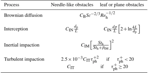
Table 1. Parameterization of the deposition efficiencies over
vege-tation.
Process Needle-like obstacles leaf or plane obstacles
Brownian diffusion CBSc−2/3Re−h1/2
Interception CIN
dp
L CINdpL
h
2+ln4dL p
i
Inertial impaction CIM
h St
h
Sth+βIM
i2
Turbulent impaction 2.5×10⁻³CITτph+2 if τ + ph<20 CIT if τph+≥20
Where ET is the total collection efficiency, and EB, EIN, EIM andEIT are the collection efficiencies corresponding to Brownian diffusion, interception, inertial impaction and turbulent impaction. In theory, these efficiencies depend on the altitude (1-D-model) but, in the present study, they are considered to have a constant value, estimated on top of the canopy (see Table 1). In order to minimize the errors induced by this simplification, the numerical coefficients appearing in the efficiency formulation are adjusted with help of the 1-D-model. This fitting procedure is detailed in Sect. 2.2.5.
Considering constant efficiencies throughout the canopy allows us to derive an analytical solution to the mass balance (Eq. 13). Introducing the non-dimensional heightz+=z/ h and concentrationγ+=γ (z)/γ (h)and accounting for the exponential profile ofKp(similar to Eq. 6), the mass balance (Eq. 13) can be rewritten as:
d2γ+ dz+2 +α
dγ+ dz+−Qγ
+=
0 with Q=h.LAI.VT Kp
. (15)
The non-dimensional number Q(as notated by Fernandez de la Mora and Friedlander, 1982) corresponds to the ratio of the turbulent transport time scale to the vegetation collection time scale. Typically,Q1 corresponds to a situation of a very efficient turbulent mixing while the transfer of particle is limited by the collection efficiency on leaves. This means an homogeneous concentration throughout the canopy, as it can be observed for Aitken and accumulation mode particles. Meanwhile,Q1 corresponds to a situation where particles are so efficiently collected by leaves that their transfer to the surfaces is rather limited by the turbulent transport. It means an inhomogeneous particle concentration within the canopy, as it can be observed for coarse mode particles. It can be rewritten as:
Q=LAIETh/ lmp(h). (16)
the flux is related to the concentration near the surfaceγ+(0) by a ground deposition velocityVg:
dγ+
dz+(0)=Qgγ +
(0) with Qg= hVg Kp0
, (17)
whereQgis the analog ofQfor the transfer to the ground, andKp0 is the value of the particle eddy diffusivity at its vicinity. The ground deposition velocity is related to the ground deposition efficiency byVg=Eguf(0). The formu-lation ofEg is based on the assumption of smooth ground and is given in Sect. 2.2.4. The non-dimensional numberQg can be rewritten as:
Qg=Egh/ lmp(h). (18)
One should note the strong similarities between the non-dimensional numbers Q and Qg, and that the amount of leaves available for deposition, i.e. LAI, is explicitly appear-ing in the formulation ofQ(Eq. 16). Assuming that the col-lection efficiencies, and thusQandQg, are constant allows us to derive an analytical solution for the particle concentra-tion:
γ+=eα/2(1−z+) "
ηcosh ηz++ Qg+α/2sinh ηz+ ηcosh(η)+ Qg+α/2sinh(η)
#
with η=
q
α2/4+Q. (19)
The deposition velocity on top of the canopy, i.e. the surface deposition velocity, corresponds to the ratio of the depositing flux on the canopy to the concentration on top of the canopy. It can be expressed as:
Vds/u∗=Vg/u∗γ0++LAIET 1 Z
0
γ+eα(z+−1)dz+. (20)
After some algebra, its formulation becomes: Vds
u∗
=Eg 1+
h
Q Qg−
α
2 i
tanh(η) η
1+Qg+α2tanhη(η)
(21)
The Eq. (21) expresses the dependency of the surface deposi-tion velocity on characteristics of the vegetadeposi-tion, the aerody-namics and the aerosol. One can thus wonder what would be the limit of the expression when the vegetation vanishes, i.e. when LAI→0 whiled/ h→0 (as prescribed by Raupach, 1994, 1995). In this case,α→0,η→0 and tanh(η)/η→1. As a consequence,Vds/u∗→Eg/(1+Qg)and the deposi-tion velocity above the canopy is such that:
1/(Vd−Vdrift)→1/(Egu∗)+h/(u∗lmp(h))+Ra(h,zR).(22) The second term on the right-hand side corresponds to the integration of 1/Kpover[0,h]whenα=0, and is equal to
Ra(0,h)(or Ra(z0,h)if we account for the roughness of the ground).
As a consequence, 1/(Vd −Vdrift) → 1/(u∗Eg)+
Ra(z0,zR), which is conform to the expectation that the surface deposition velocity for bare ground is driven by the deposition efficiency on the ground and the aerodynamic resistance.
2.2.3 Surface deposition velocity for non-vegetated surfaces
By extension of the asymptotic limit of Eq. (21) without veg-etation, the deposition velocity for non-vegetated surfaces (liquid or solid water surfaces and desert) is simply:
Vd(zR)=Vdrift+
1
Ra(z0,zR)+1/(Egu∗)
(23)
where the expression ofEgis detailed hereafter. 2.2.4 Parameterization of the ground deposition The aerosol deposition on the ground below the vegetation canopy takes into account the Brownian diffusion and the tur-bulent impaction. Their deposition efficiencies, respectively Egb andEgt, are based on theoretical and empirical results obtained for turbulent flow in pipes (see for example Davies, 1966; Papavergos and Hedley, 1984). The Brownian diffu-sion efficiency is expressed as:
Egb=
Sc−2/3
14.5 "
1 6ln
(1+F )2 1−F+F2+
1
√
3Arctan 2F−1
√
3
+ π
6
√
3 #−1
,
(24) whereF is a function of the Schmidt number expressed as F=Sc1/3/2.9. An approximation of Eq. (24) given by Wood (1981) has been used by Petroff et al. (2009). However in the present study we prefer to use the original formulation rather than the simplification proposed by Wood, because the latter leads to significant errors for nano-particles: At 20◦C, the relative error is about 60% for 1 nm particles while it falls to about 5% for 14 nm particles.
The turbulent impaction efficiency term is similar to the one used to model deposition on vegetation (see Table 1) but is expressed on the ground, i.e. for a local friction velocity of uf=u∗e−α. The constantCITis taken as 0.14. The latter is slightly different than previous work (0.18) but ensures the continuity ofEITwhenτp+=20. This change does not affect the results of the 1-D-model in a significant way.
2.2.5 Parameterization of the collection efficiencies on leaves
operational perspective, where such morphological and sta-tistical details are out of reach, these dependencies are sim-plified in the following ways. The characteristic lengthLof the canopy obstacles is taken as the diameter for needles and as the mean width for leaves. It follows a Dirac distribution i.e. each obstacle has the same size. A uniform distribution is assumed for the azimut angle. The inclination distribu-tion is chosen as vertical for short grass, as erectophile for long grass and all crop species, while forests and shrubs are described by the plagiophile distribution. Boundary-layers around obstacles are assumed to be laminar. The correspond-ing formulations of the efficiencies are based on the 1-D-model. They are briefly restated in Table 1, where Sc is the Schmidt number (Sc=νa/DB,DBbeing the coefficient of Brownian diffusion and νa air kinematic viscosity), Reh is the Reynolds number of the flow estimated on top of the canopy (Reh=UhL/νa, Sth is the Stokes number on top of
the canopy (Sth=τpUh/L, withτpthe relaxation time of the particle),τph+ is the non-dimensional relaxation time of the particle on top of the canopy (τph+=τpu2∗/νa).
In theory, the constantsCB,CIN,CIM andCITappearing in Table 1 account for the chosen distributions of charac-teristic length and orientation of the obstacles. But in the present model, the efficiencies are taken constant throughout the canopy and the different constants have to be adjusted for each vegetated surfaces.
To do so, in a first step, probable variation ranges are de-fined for the main parameters of the two models, namely the friction velocity (3 values), the obstacle dimension (2 values), the ratios z0/ h (0.05–0.1) and d/ h (0.65–0.85), LAI (2 values), particle density (1000–3000 kg m−3) and the ratio of the foliage base height to the canopy heights (2 values, only for forest and shrubs). The combinations of these parameters gives us between 96 and 192 configu-rations. In a second step, the present model and the 1-D-model are run side by side under each of these configura-tions for particle size between 1 nm and 1 mm. The relative error between them, Err, is used to estimate their agreement: Err=(Vd(1-Dmodel)−Vd(present))/Vd(1-D-model). Mul-tiple values of the coefficientsCB,CIN,CIMandCITare used to run the present model until the relative error with the 1-D-model is minimized over the entire size range.
Such a fitting exercise is required for two reasons. The first is that the derivation of the present model assumes constant particle deposition efficiencies. The second reason is that the present model treats the vegetation surface as vertically uni-form. This assumption induces biases with the 1-D-model in canopies such as forest, in which vegetation is concentrated in the upper-part of the canopy where the wind is strong. The values ofCB, CIN, CIM andCIT resulting from this fitting procedure are given in Table 2.
In order to control the quality of the fit of the different con-stants, we consider the land cover 14, i.e. long grass, and we study the contributions of the different processes to the total
deposition predicted by the present model (see Fig. 1). The relative error between the present model and the 1-D-model is also given, when processes are considered separately or together (see Fig. 1, right hand side).
Under low wind, the deposition of particle is driven by Brownian diffusion, interception and sedimentation (see Fig. 1a). There, one can notice an under-estimation of the present model for coarse particles that is due to the treatment of the gravity. In the present model, sedimentation is con-sidered independently of the amount of vegetation surfaces and their orientation, while in the 1-D-model, the sedimen-tation is considered as a collection mechanism both on the leaves and the canopy ground. As a result, the sedimenta-tion is under-estimated in the present model. As the wind increases, this effect vanishes because sedimentation is not the sole dominant process anymore in this size range and that other effects related to particle inertia (inertial and turbulent impactions) become important too (see Fig. 1d). The relative error between the two models, when only one process is ac-tivated, can be significant, in particular for inertial effects on fine particles. However, this gap does not have an impact on the overall prediction, because these processes are not domi-nant in this particular size range. In general, the relative error remains smaller than 30%, which confirms the quality of the fit.
0.001 0.01 0.1 1 10 100
0.01 0.1 1 10 100
Deposition velocity (cm.s
-1)
diameter (micron) (a) Vd at u* = 10 cm.s
-1
Brownian diffusion Interception Inertial impaction Turbulent impaction Sedimentation All processes
-40 -20 0 20 40 60 80 100
0.01 0.1 1 10 100
Relative error (%)
diameter (micron) (b) Err at u*=10 cm.s
-1
0.001 0.01 0.1 1 10 100
0.01 0.1 1 10 100
Deposition velocity (cm.s
-1)
diameter (micron) (c) Vd at u* = 90 cm.s-1
-40 -20 0 20 40 60 80 100
0.01 0.1 1 10 100
Relative error (%)
Diameter (micron) (d) Err at u* = 90 cm.s-1
Fig. 1. Deposition on long grass (LUC 14) and influence of the different processes under low and wind high conditions (u∗=10 and
90 cm s−1). The canopy is characterized byh=0.77 m, LAI=4,z0=0.1 m andd=0.49 m, whileρp=1500 kg m−3. The deposition
velocity atzR=5 m, predicted by the present model, is given on the left hand side. The relative error Err between the present model and the
1-D-model is given on the right hand side, when the different processes are considered separately or together.
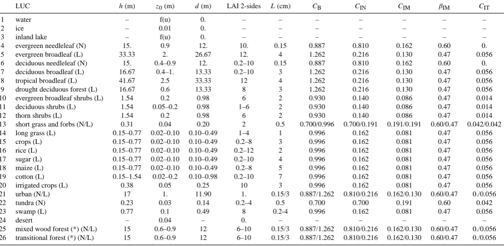
Table 2. Coefficients for different Land Use Categories (LUC). The obstacle shape chosen to represent the LUC is given in brackets as N
for needle and L for leaf or plane obstacles. (*) For the mixed wood forest and transitional forest, the deposition velocity for the evergreen needleleaf forest (LUC 4) and for the deciduous broadleaf forest (LUC 7) are calculated and the resulting deposition velocity for the mixed wood forest and the transitional forest is estimated as the average weighted by the proportion of tree types.
LUC h(m) z0(m) d(m) LAI 2-sides L(cm) CB CIN CIM βIM CIT
1 water – f(u) 0. – – – – – – –
2 ice – 0.01 0. – – – – – – –
3 inland lake – f(u) 0. – – – – – – –
4 evergreen needleleaf (N) 15. 0.9 12. 10. 0.15 0.887 0.810 0.162 0.60 0. 5 evergreen broadleaf (L) 33.33 2. 26.67 12. 4 1.262 0.216 0.130 0.47 0.056 6 deciduous needleleaf (N) 15. 0.4–0.9 12. 0.2–10 0.15 0.887 0.810 0.162 0.60 0. 7 deciduous broadleaf (L) 16.67 0.4–1. 13.33 0.2–10 3 1.262 0.216 0.130 0.47 0.056 8 tropical broadleaf (L) 41.67 2.5 33.33 12 4 1.262 0.216 0.130 0.47 0.056 9 drought deciduous forest (L) 16.67 0.6 13.33 8 3 1.262 0.216 0.130 0.47 0.056 10 evergreen broadleaf shrubs (L) 1.54 0.2 0.98 6 2 0.930 0.140 0.086 0.47 0.014 11 deciduous shrubs (L) 1.54 0.05–0.2 0.98 1–6 2 0.930 0.140 0.086 0.47 0.014
12 thorn shrubs (L) 1.54 0.2 0.98 6 2 0.930 0.140 0.086 0.47 0.014
13 short grass and forbs (N/L) 0.31 0.04 0.20 2 0.5 0.700/0.996 0.700/0.191 0.191/0.191 0.60/0.47 0.042/0.042 14 long grass (L) 0.15–0.77 0.02–0.10 0.10–0.49 1–4 1 0.996 0.162 0.081 0.47 0.056 15 crops (L) 0.15–0.77 0.02–0.10 0.10–0.49 0.2–8 3 0.996 0.162 0.081 0.47 0.056 16 rice (L) 0.15–0.77 0.02–0.10 0.10–0.49 0.2–12 2 0.996 0.162 0.081 0.47 0.056 17 sugar (L) 0.15–0.77 0.02–0.10 0.10–0.49 0.2–10 4 0.996 0.162 0.081 0.47 0.056 18 maize (L) 0.15–0.77 0.02–0.10 0.10–0.49 0.2–8 5 0.996 0.162 0.081 0.47 0.056 19 cotton (L) 0.15–1.54 0.02–0.2 0.10–0.98 0.2–10 7 0.996 0.162 0.081 0.47 0.056
20 irrigated crops (L) 0.38 0.05 0.25 10 3 0.996 0.162 0.081 0.47 0.056
21 urban (N/L) 17 1. 11.90 1. 0.15/3 0.887/1.262 0.810/0.216 0.162/0.130 0.60/0.47 0./0.056
22 tundra (N) 0.23 0.03 0.14 0.2–4 0.5 0.700 0.700 0.191 0.60 0.042
23 swamp (L) 0.77 0.1 0.49 8 0.2-4 0.996 0.162 0.081 0.47 0.056
24 desert – 0.04 – 0. – – – – – –
the buildings. The assumption here is that particle deposi-tion is only significant over extended vegetadeposi-tion areas such as parks and that at the city scale, particle emission, accounted for in another module of the chemical transport model, is significantly dominating the aerosol balance (see the mea-surements by Dorsey et al., 2002; M˚artensson et al., 2006; Schmidt and Klemm, 2008).
3 Results
Results of the present model are evaluated in the following manner. First, its results are compared with the results of the 1-D-model on two typical vegetated canopies, in order to ensure the quality of the fit. Secondly, its results are com-pared to measurements obtained for different earth surfaces, such as desert, short grass, coniferous forest and water, both in liquid and solid phases as well as results produced by the model of Zhang et al. (2001). Unless otherwise stated, the aerosol density is chosen asρp=1500 kg m−3.
It is worth mentioning at this point the main differences between the present model and Zhang et al.’s model: First, the formulation of the surface deposition velocity is differ-ent and the presdiffer-ent model accounts for more morphological characteristics of the canopy such as the leaf area index LAI and the canopy height. The sensitivity to surface change is thus expected to be larger in the present model. Secondly, the same processes are considered here and in Zhang et al.’s model, except the rebound, not accounted for in the present model and the turbulent impaction, accounted here but not in Zhang et al.’s model. For processes described in both models, the parameterization is significantly different (see for exam-ple the Brownian diffusion). Thirdly, in the present model, the ground is explicitly accounted for as a deposition surface of the land cover. As a result, bare ground appears as an asymptotic case when the canopy vegetation vanishes. 3.1 Evaluation of the fit on two vegetation covers Two typical vegetation covers of short grass (LUC 13) and coniferous forest (LUC 4) are chosen to compare in Fig. 2 the present model and the 1-D-model. The relative error is used as an indicator of agreement and different wind conditions are explored.
On these vegetation covers, the relative error stays con-fined between−30 and 25%. One should notice that it re-turns to 0 when the particle diameter increases and that the sedimentation dominates the deposition.
The difference of treatement of the gravity appears for the coniferous forest under very light wind conditions (see Fig. 2d). There, the visible under-estimation of the aggre-tated model for particle between 1 and 10 µm is related to the fact that the inclinated leaves (plagiophile distribution) col-lect particles by gravity in the 1-D-Model. Meanwhile, the present model does not account for sedimentation as a
col-lection mechanism on the vegetation per se, but rather con-siders it as a process of deposition on the overall surface. For stronger wind, this bias disappears quickly.
3.2 Deposition on bare soil
We rely on experimental measurements of deposition on a smooth horizontal surface (Sehmel, 1973) to assess the va-lidity of the parameterization of the ground deposition and evaluate the present model on bare soil/desert (Eq. 23). The Fig. 3 presents the evolution of the deposition velocity at zR=1 m with particle diameter for three different flow con-ditions. Results of Zhang et al.’s model are also included on Fig. 3.
Under conditions of low wind (u∗=11 cm s−1), the
de-position of coarse particles is strictly driven by the effect of gravity and both models reproduce this effect properly and stick to the curve of sedimentation. As the friction veloc-ity increases, inertial effects are taking place for particles larger than 2 microns, which are correctly accounted for in both models (by a maximum factor of 2). Larger differences between models arise in the accumulation mode, where the present model reproduces adequately these measurements while Zhang et al’s model over-estimates them by one to two orders of magnitude. The reason of this broad difference be-tween models lies in the parameterization of the Brownian diffusion, in particular a difference of one order magnitude in the numerical constant and of one tenth in the Schmidt number exponent.
One can also notice on Fig. 3 the impact of the surface stickiness on the deposition of the coarsest particles by strong wind (last point of the data set corresponding todp=30 µm). The rebound, not accounted for in the present model, induces an over-estimation of a factor 4.
It is important to mention that real bare ground differs from this ideal smooth situation in which the measurements have been performed. The increase of roughness related to the topography and the presence of bulk obstacles like rocks or isolated plants most likely will perturbate the flow and the deposition pattern. More measurements are needed to esti-mate the expected increase in the deposition velocity of fine particles and improve the parameterization of the ground de-position.
3.3 Deposition on short grass
Experiments performed on short grass (Chamberlain, 1967; Clough, 1975; Garland, 1983) and moorland (Gallagher et al., 1988; Nemitz et al., 2002) are used to evaluate the per-formance of the present model fed with the parameters of LUC 13 (Tables 1 and 2). The two possible shapes of obsta-cle (plane or cylindrical) are investigated. The present model, the 1-D-model and the model of Zhang et al. (2001) are run for a friction velocity ofu∗=40 cm s−1, which corresponds
0.01 0.1 1 10 100
0.01 0.1 1 10 100 -50 -25 0 25 50
Deposition velocity (cm.s
-1)
relative error (%)
diameter (micron)
Short leaf grass a) u* = 10 cm.s -1
WS
1D-model Present model Relative error
0.01 0.1 1 10 100
0.01 0.1 1 10 100 -50 -25 0 25 50
b) u* = 50 cm.s -1
0.01 0.1 1 10 100
0.01 0.1 1 10 100 -50 -25 0 25 50
c) u* = 90 cm.s -1
0.01 0.1 1 10 100
0.01 0.1 1 10 100 -50 -25 0 25 50
Deposition velocity (cm.s
-1)
relative error (%)
diameter (micron)
Needle forest d) u* = 10 cm.s -1
0.01 0.1 1 10 100
0.01 0.1 1 10 100 -50 -25 0 25 50
e) u* = 50 cm.s -1
0.01 0.1 1 10 100
0.01 0.1 1 10 100 -50 -25 0 25 50
f) u* = 90 cm.s -1
Fig. 2. Comparison of the present model and the 1D-model under configurations of evergreen needleleaf
forest (LUC 4) and short grass (LUC 13, with leaves) for different friction velocity conditions. For the 1D-model, the crown base height of the forest is taken as h/2and the vertical profile of the leaf surface density as gaussian. Other parameters are given in Table 2. Blue and red plain lines correspond respectively to the present model and the one-dimensional model, while the green plain line corresponds to the relative error between them. The black line corresponds to the sedimentation velocity.
3.2
Deposition on bare soil
We rely on experimental measurements of deposition on a smooth horizontal surface (Sehmel,
1973) to assess the validity of the parameterization of the ground deposition and evaluate the
22
Fig. 2. Comparison of the present model and the 1-D-model under configurations of evergreen needleleaf forest (LUC 4) and short grass
(LUC 13, with leaves) for different friction velocity conditions. For the 1-D-model, the crown base height of the forest is taken ash/2 and the vertical profile of the leaf surface density as gaussian. Other parameters are given in Table 2. Blue and red plain lines correspond respectively to the present model and the the 1-D-model, while the green plain line corresponds to the relative error between them. The black line corresponds to the sedimentation velocity.
0.001 0.01 0.1 1 10 100
0.01 0.1 1 10 100
Vd
(cm.s
-1) at 1m
dp (micron)
WS
u*=11 cm.s-1
u*=34 cm.s-1
u*=73 cm.s -1
sticky u*=73 cm.s -1
Fig. 3. Deposition on smooth soil, as measured through its mean
and standard deviation by Sehmel (1973) and predicted by the present model and the model of Zhang et al. (2001), respectively in plain and dashed lines, for friction velocities of 11 cm s−1(blue), 34 cm s−1(red), 74 cm s−1(green).
(u∗∈ [25;55 cm s−1]). The atmosphere is assumed to be in
near-neutral condition. A common height of 3.8 m is used to recalculate the deposition velocity (Eq. 10). Results are presented on Fig. 4.
0.001 0.01 0.1 1 10 100
0.01 0.1 1 10 100
Vd
(cm.s
−1
) at 3.8m
dp (micron) WS
Moorland: Nemitz 2002 Moorland: Gallagher 1988 Grass: Clough 1975 Sticky grass: Chamberlain 1967 Grass: Chamberlain 1967 Zhang 2001 1D−model leaf needle Present model leaf needle
Fig. 4. Deposition on grass, as measured by Chamberlain (1967);
Clough (1975); Garland (1983); Gallagher et al. (1988); Nemitz et al. (2002) for friction velocity between 25 and 55 cm s−1. A fric-tion velocity of 40 cm s−1is used to run the model of Zhang et al. (2001, in brown), the 1-D-model on leaf and needle obstacles (red plain and dash) and the present model on leaf and needle obstacles (blue plain and dash). All deposition velocities are re-calculated at
zR=3.8 m. The particle density is taken asρp=1500 kg m−3.
shape and obstacle size,z0/ h,d/ h) as well as wind condi-tions have been proven to have a strong impact on the deposi-tion (Davidson et al., 1982; Petroff et al., 2009, in particular Fig. 14 of the latter). The shape of the obstacle is showed here to have a significant impact on the deposition too. Let every other parameter be the same, the deposition on grass composed of plane obstacles is larger than on grass com-posed of cylindrical obstacles. The difference can reach a factor 3 for accumulation mode particles. The reason for such a difference is to find in the different aerodynamics around a plane obstacle and around a cylinder (within the boundary-layer and above). As a result, the deposition ef-ficiencies associated with Brownian diffusion, interception and impaction depend strongly on the obstacle shape.
This comparison with measurements indicates rea-sonnable behaviours of both the leaf and the needle versions of the present model for any particle size. The model of Zhang et al. (2001) agrees with data for particle larger than some tenths of microns, but over-estimates the deposition of the smaller ones, due to its parameterization of the Brownian diffusion.
3.4 Deposition on coniferous forests
A similar comparison is performed on forests of differ-ent coniferous species: spruce (Beswick et al., 1991), pine (Lorenz and Murphy, 1989; Lamaud et al., 1994; Buzorius et al., 2000; Gaman et al., 2004; Gr¨onholm et al., 2009) and fir (Gallagher et al., 1997). In these experiments, the friction velocity varies between 35 and 60 cm s−1and the atmosphere is in a near-neutral condition. Models were fed with param-eters of LUC 4 with a friction velocity ofu∗=47.5 cm s−1.
All deposition velocities are recalculated at twice the canopy height, i.e.zR=30 m (see Fig. 5).
Generally speaking, a good agreement is found between these measurements and the present model, though some dis-crepancies arise in the case of coarse fog droplets depositing on low spruce (measured by Beswick et al., 1991). The rea-son is that the conditions of this particular experiment are slightly different from the ones used to run the model, in particular the friction velocity is smaller (u∗=37 cm s−1
in-stead ofu∗=47.5 cm s−1) and the aerosol is less dense (ρp= 1000 kg m−3instead of 1500 kg m−3). These changes cause a lower deposition than predicted by the model in the typi-cal coniferous situation. One can verify that by running the model with the exact parameters of Beswick et al.’s experi-ment (represented as a dashed blue line on Fig. 5), in which case the agreement between the model and the measure-ments is improved. Interestingly, the model of Zhang et al. (2001) agrees relatively well with most of these measure-ments, Aitken mode excepted, where it likely over-estimates the measurements by a factor 4 or more.
0.001 0.01 0.1 1 10 100
0.01 0.1 1 10 100
Vd
(cm.s
−1
) at 30m
dp (micron)
WS (ρp=1500 kg.m −3)
WS (ρp=1000 kg.m−3)
Low Spruce: Beswick 1991 Pine: Lorenz 1989 Pine: Lamaud 1994 Pine: Buzorius 2000 Pine: Gaman 2004 Pine: Grönholm 2009
Fir: Gallagher 1997 Zhang 2001
1D−model Present model
Fig. 5. Deposition on coniferous forest, as measured by Beswick
et al. (1991); Lorenz and Murphy (1989); Lamaud et al. (1994); Bu-zorius et al. (2000); Gaman et al. (2004); Gr¨onholm et al. (2009); Gallagher et al. (1997). A friction velocity of 47.5 cm s−1, a particle density of 1500 kg m−3and the parameters of the LUC 4 are used to run the model of Zhang et al. (2001, in plain brown), the 1-D-model (in plain red) and the present model (in plain blue). Are added in blue dots the predictions of the present model obtained under the configuration of Beswick et al.’s experiment: u∗=37 cm s−1, h=4.2 m, hc=1 m, LAI=10,z0=0.3 m andd=2.8 m,ρp=
1000 kg m−3. All deposition velocities are re-calculated at zR=
30 m.
3.5 Deposition over liquid water surfaces
We want to estimate the ability of this simple model (Eq. 23) to reproduce measurements on liquid water surfaces. Differ-ent campaigns in wind-tunnel (M¨oller and Schumann, 1970; Sehmel and Sutter, 1974) and on lake (Zufall et al., 1998; Caffrey et al., 1998) are used for this purpose. The relation-ship between the wind and the modification of the surface morphology (waves) is accounted for according to Charnock (1955) and Smith (1988). Under neutral conditions, mean wind, friction velocity and roughness length are related by:
z0=0.11νa/u∗+0.011u2∗/g and
u∗=κU (zR)/ln(zR/z0). (25)
This equation is used to calculate by iteration the friction velocity and the roughness length from the wind velocity. On the Fig. 6, we present together the results of the present model and the model of Zhang et al. (2001). All deposition velocity are recalculated atzR=5.2 m using the Eq. (10). Three wind regimes are represented on Fig. 6 with different colors: blue for low wind (u∗=11 cm s−1), red for
inter-mediate wind (u∗=44 cm s−1), and green for strong wind
(u∗=117 cm s−1).
0.001 0.01 0.1 1 10 100
0.01 0.1 1 10 100
Vd
(cm.s
−1
) at 5.2m
dp (micron)
Vphor=0.005 cm.s−1
WS
Möller 1970: u*=40 cm.s−1
Sehmel 1974: u*=11 cm.s−1
u*=44 cm.s−1
u*=117 cm.s−1
Zufall 1998: u*=11−18 cm.s−1
Caffrey 1998: u*=11−16 cm.s−1
Fig. 6. Deposition on water surfaces, as measured by M¨oller and
Schumann (1970); Sehmel and Sutter (1974); Zufall et al. (1998); Caffrey et al. (1998). The present model (plain) and the model of Zhang et al. (2001, dash) are run foru∗=11 cm s−1 (blue), u∗=44 cm s−1(red) andu∗=117 cm s−1(green). All deposition
velocities are re-calculated atzR=5.2 m. The particle density is
taken asρp=1500 kg m−3.
allows us to reproduce well these data. For stronger wind, the Brownian diffusion becomes efficient as the particle size de-creases, which the present model is able to reproduce with a slight under-estimation (see the data of M¨oller and Schu-mann, 1970). The model of Zhang et al. (2001) significantly over-estimates the measurements for this size range, which is due to the parameterization of the Brownian diffusion effi-ciency (see the discussion on bare ground).
The deposition of coarser particles is driven by gravity when the wind is low and by gravity and turbulent impaction as the friction velocity increases. In most situations, a rea-sonable agreement is reached between the measurements and both the displayed models in low or strong winds. Some dif-ferences arise though for stronger winds and particles around 5–10 µm, for which an under-estimation of the present model is noticed (in most cases of a factor 2).
We emphasize that none of the measurements used in the present comparison reflects the situation of an ocean or a sea, where previous works expect an impact of spray formation on particles deposition under strong wind condi-tions (Williams, 1982; Hummelshøj et al., 1992; Pryor and Barthelmie, 2000). More experiments are needed to assess this effect, using preferably direct eddy-correlation measure-ments (see for example Norris et al., 2008).
3.6 Deposition over snow and ice surfaces
Snow and ice represent a significant portion of the earth sur-face and require to be adequately taken into account in trans-port models. Despite the imtrans-portance of these surfaces, the di-rect measurements of aerosol fluxes providing as well some information about the aerosol size are sparse, relatively to
0.001 0.01 0.1 1 10 100
0.01 0.1 1 10 100
Vd
(cm.s
−1) at 10m
dp (micron) WS
Vphor=0.02 cm.s−1
Ibrahim 1983 u*=16 cm.s−1
Duan 1988 u*=12 cm.s−1
Nilsson 2001 u*=18 cm.s−1
Contini 2010 u*=11 cm.s−1 Present Model u*=17 cm.s−1
u*=36 cm.s−1
Zhang 2001 u*=17 cm.s−1
u*=36 cm.s−1
Fig. 7. Deposition on snow and ice surfaces, as measured by
Ibrahim et al. (1983); Duan et al. (1988); Nilsson and Rannik (2001); Contini et al. (2010). The present model (plain) and the model of Zhang et al. (2001, dash) are run foru∗=17 cm s−1
(blue) andu∗=36 cm s−1(red) for an air temperature of 273◦K
(0◦C) andz0=10−3m. All deposition velocities are re-calculated
atzR=10 m. The particle density is taken asρp=1500 kg m−3.
liquid water surfaces. They are obtained on snow (Ibrahim et al., 1983; Duan et al., 1988) and ice (Nilsson and Ran-nik, 2001; Contini et al., 2010) and the roughness length varies between 10−4and 2×10⁻²m (Nilsson et al. measured roughness length up to 0.3 m – 90 percentile – over rough ice floes). The data presented here as (Contini et al., 2010) cor-respond to 20 near-neutral periods over which the size distri-bution and flux is measured simultaneously. The predictions of the present model and of the model of Zhang et al. (2001) are compared with these experiments on Fig. 7.
One should mention that the symbols and “error” bars do not represent on the Fig. 7 the same quantities. Deposition velocity is given as a mean and a standard deviation, excepted for Nilsson and Rannik (2001), for which the bar corresponds to the minimum and maximum values obtained over two un-known numbers of periods where size distributions are “typ-ical” of ultra-fine or Aitken particles. Neither has the “error” bar on the particle diameter the same meaning in these differ-ent campaigns: Ibrahim et al. (1983) and Nilsson and Rannik (2001) do not report the meaning of these bars in their graphs. In the study of Duan et al. (1988), the bar correspond to the size bins detected by the optical counters. Finally, for the Antartica campaign of Contini et al. (2010), the bar corre-sponds in the present paper to the size range where 85% of the number concentration is located.
Based on these few and quite uncertain measures, the drift velocity corresponding to phoretic effects on ice and snow is chosen as 2×10⁻⁴cm s−1.
One interesting feature here is that deposition of fine par-ticles appears to be larger over snow and ice than on wa-ter (compare with Fig. 6). In an effort to inwa-terpret their re-sults, Ibrahim et al. (1983) invoke strong humidity gradients close to the snow ground that would affect ammonium sulfate particles and allow them to grow by hygroscopicity. The rea-son to explain that such behaviour would not be experienced on liquid water is unclear. Experiments over longer periods of time and with simultaneous measures of the humidity and temperature gradients close to the ground would be useful to firmly evaluate the validity of the present model on ice and snow surfaces.
4 Conclusions and perspectives
In the present paper, we proposed an analytical model to pre-dict the deposition of aerosols of different sizes on the earth surface. It updates the model of Zhang et al. (2001) and de-pends on the morphology of the surface cover, the aerody-namics and the aerosol properties. On top of classical sur-face parameters like the leaf size, other factors such as the leaf shape, leaf area index and canopy height are now ex-plicitly accounted for. This induces a larger sensitivity of the present model to changes of the land cover, compared to the earlier model (see Figs. 2 and 4). This model has been compared with measurements and gives reasonable re-sults for bare ground (taken as a smooth surface, see Fig. 3), for different vegetation covers (short grass, see Fig. 4, and coniferous forest, see Fig. 5) and for liquid water surface (see Fig. 6). Comparatively, Zhang et al.’s model, developed at a time when measurements were sparse and incomplete, tends to adequately predict the deposition of coarse mode parti-cles on the land covers examined in the present paper. The situation for other particle modes is more contrasted. The deposition on coniferous forest of the accumulation mode is adequately predicted while the Aitken mode measurements are over-estimated by their model. Over less rough surfaces, the deposition of fine particles is over-estimated by Zhang et al.’s model by one or two orders of magnitude. This is due to the combined limited sensitivity of their model to surface change and the parameterization of the Brownian diffusion.
Consistently with recent reviews (Pryor et al., 2008; Petroff et al., 2008a), the deposition over coniferous forest is predicted by the present model to be larger than over grass (see Fig. 2). This increase, depending on the flow and canopy properties, can reach one order of magnitude in the accumu-lation and coarse modes. Comparatively, the increase pre-dicted by Zhang et al.’s model between grass and forest con-figuration is lower and mainly regards the coarse mode (fac-tor of 4–5).
Based on the reviewed measurements, the minimum of de-position velocity is thought to be in the accumulation mode, which the present model is able to predict, while Zhang et al.’s model predicts it for particles around 1 or 2 microns.
In order to complete the validation of the present model, future work should focus on the influence of the stability. A simple way to account for it within the canopy has been proposed in the present study but still needs to be confronted to experimental results.
Different perspectives of improvement of this model are considered. The first regards the parameterization of the ground deposition, which in the present study is assumed to be a smooth surface. The roughness increase due to the topography and the presence of bulk obstacles like rocks or isolated plants will perturbate the flow and increase the de-position. This boundary condition needs to be improved in the future, as detailed measurements on real and rough bare ground become available.
Secondly, the phoretic effects induced by humidity and temperature gradients above solid and liquid water surfaces are described here by a simple constant drift velocity. The value of this drift velocity has been adjusted in the present study on existing measurements. As more data will be-come available, it should be modified or replaced by a proper paramerization. Ideally, experiments would cover particle flux and growth as well as temperature and humidity profiles close to the surface.
Thirdly, the rebound and the resuspension could be in-cluded in the future when one would be able to inform the characteristics of the deposition surface (micro-roughnesses, humidity) and the state of the aerosol and to derive simple enough formulations of these complex processes.
A fourth perspective regards processes, such as gas-particle and gas-particle-gas-particle interactions or gas-particle emis-sion, that can modify the flux balance above the canopy. Even if these processes likely are accounted for in other mod-ules of the chemical transport model, model prediction might gain from the inclusion in the same module of all the interac-tions occurring between the surface and the aerosol and gas phases.
The present model is available as a open source Fortran90 routine and can be obtained from the authors.
Appendix A Notations
CC Cunningham correction fac-tor CC=1+2λ/dp(1.257+ 0.400e−1.1dp/(2λ))
[–]
DB Brownian diffusivity DB= CCkBT /(3π µadp)
[m2s−1] ET,EB,
EIN,EIM
Deposition efficiencies on the foliage
[–] Eg Deposition efficiency to the
ground
Kp Particle eddy diffusivity [m2s−1]
L Obstacle characteristic
dimension
[m]
LO Obhukov length [m]
LAI Two-side leaf area index [–] Q,Qg non-dimensional
num-bers
[–]
Ra Aerodynamic resistance [s m−1]
Reh Reynolds number on top of the canopy
[–]
Sc Schmidt number [–]
Sth Stokes number on top of the canopy
[–]
T Temperature, taken as
293, if not otherwise stated
[K]
U Horizontal mean flow
velocity
[m s−1] Vd Deposition velocity [m s−1] Vdrift Drift velocity [m s−1] Vg ground deposition
veloc-ity
[m s−1] Vphor phoretic drift velocity [m s−1] VT total collection velocity
on vegetation
[m s−1] WS sedimentation velocity
WS=gτp
[m s−1]
a Two-side leaf area
den-sity
[m−1]
d displacement height [m]
dp particle diameter [m]
g gravity acceleration [m s−2]
h mean canopy height [m]
hc mean height of the crown base
[m] kB Boltzman constant kB=
1.38×10⁻²³
[J K−1] kx inclination coefficient of
the canopy elements
[–] lmp mixing length for
parti-cles
[m] uf local friction velocity [m s−1]
u∗ friction velocity [m s−1]
z0 roughness length [m]
κ Von K¨arman constant [–]
9m,9h integrated forms of the stability function for mo-mentum and heat
[–]
φh stability function for heat [–]
α aerodynamic extinction
coefficient
[–]
γ aerosol mass
concentra-tion density
[kg m−4]
η non-dimensional number [–]
λ mean free path of airλ= [m]
µa air dynamic viscosity
µa=1.89×10⁻⁵
[kg m−1s−1] νa air kinematic viscosity
νa=1.57×10⁻⁵
[m2s−1] τp+ non-dimensional particle
relaxation time
[–] τp particle relaxation time
τp=CCρpdp2/(18µa)
[s]
ρp particle density [kg m−3]
Acknowledgements. Daniele Contini is acknowledged for sharing
with us the aerosol data obtained in Antartica. Edited by: R. Sander
References
Andersson, C., Langner, J., and Bergstr¨om, R.: Interannual varia-tion and trends in air polluvaria-tion over Europe due to climate vari-ability during 1958–2001 simulated with a regional CTM cou-pled to the ERA40 reanalysis, Tellus, 59B, 77–98, 2007. Bache, D.: Particle transport within plant canopies. I. A framework
for analysis, Atmos. Environ., 13, 1257–1262, 1979.
Batchelor, G. and Shen, C.: Thermophoretic deposition in gas flow over cold surfaces, Journal of Colloid Interface Science, 107, 21– 37, 1985.
Bessagnet, B., Hodzic, A., Vautard, R., Beekmann, M., Cheinet, S., Honor´e, C., Liousse, C., and Rouil, L.: Aerosol modelling with CHIMERE-preliminary evaluation at the continental scale, Atmos. Environ., 38, 2803–2817, 2004.
Beswick, K., Hargreaves, K., Gallagher, M., Choularton, T., and Fowler, D.: Size-resolved measurements of cloud droplet depo-sition velocity to a canopy using an eddy correlation technique, Q. J. Roy. Meteorol. Soc., 117, 623–645, 1991.
Brunet, Y., Finnigan, J., and Raupach, M.: A wind Tunnel study of Air Flow in Waving Wheat: Single point velocity statistics, Bound.-Lay. Meteorol., 70, 95–132, 1994.
Buzorius, G., Rannik, ¨U., M¨akel¨a, J., Vesala, T., and Kulmala, M.: Vertical aerosol fluxes measured by eddy covariance methods and deposition of nucleation mode particles above a Scots pine forest in southern Finland, J. Geophys. Res., 105, 19905–19916, 2000.
Caffrey, P., Ondov, J., Zufall, M., and Davidson, C.: Determination of size-dependent dry particle deposition velocities with multiple intrisic elemental tracers, Environ. Sci. Technol., 32, 1615–1622, 1998.
Cellier, P. and Brunet, Y.: Flux-gradient relationships above tall plant canopies, Agr. Forest Meteorol., 58, 93–117, 1992. Chamberlain, A.: Transport of Lycopodium spores and other small
particles to rough surfaces, Proceedings of the Royal Society London, 296, 45–70, 1967.
Charnock, H.: Wind stress on a water surface, Q. J. Roy. Meteorol. Soc., 81, 639–640, 1955.
Clough, W.: The deposit of particles on moss and grass surfaces, Atmos. Environ., 9, 1113–1119, 1975.
Nansen Ice Sheet (Antartica), J. Geophys. Res., 115, D16202, doi:10.1029/2009JD013600, 2010.
Cˆot´e, J., Gravel, S., M´ethot, A., Patoine, A., Roch, M., and Stan-iforth, A.: The operational CMC-MRB Global Environmental Multiscale (GEM) model. Part I: Design considerations and for-mulation, Mon. Weather Rev., 126, 1373–1395, 1998.
Davidson, C., Miller, J., and Pleskow, M.: The influence of sur-face structure on predicted particle dry deposition to natural grass canopies, Water, Air and Soil Pollution, 18, 25–43, 1982. Davies, C.: Deposition from moving aerosols, in: Aerosol science,
edited by Davies, C. N., pp. 393–446, Academic Press, London, UK, 1966.
Denmead, O. and Bradley, E.: Flux-gradient relationships in a for-est canopy, in: The Forfor-est-Atmosphere Interaction, edited by: Hutchinson, B. and Hicks, B. B., pp. 421–442, D. Reidel Pub-lishing Company, Dordrecht, 1985.
Dickinson, R. E., Henderson-Sellers, A., Kennedy, P. J., and Wilson, M. F.: Biosphere-Atmosphere Transfer Scheme (BATS) for the NCAR Community Climate Model, Tech. Rep. NCAR/TN275+STR, National Centre for Atmospheric Re-search, Boulder, Colorado, 1986.
Dorsey, J., Nemitz, E., Gallagher, M.W. Fowler, D., Williams, P., Bower, K., and Beswick, K.: Direct measurements and param-eterisation of aerosol flux, concentration and emission velocity above a city, Atmos. Environ., 36, 791–800, 2002.
Duan, B., Fairall, C., and Thomson, D.: Eddy-correlation measure-ments of the dry deposition of particles in wintertime, J. Appl. Meteorol., 27, 642–652, 1988.
Dyer, A.: A review of flux-profile relationships, Bound.-Lay. Mete-orol., 7, 363–372, 1974.
Englert, N.: Fine particles and human health - a review of epidemi-ological studies, Toxicol. Lett., 149, 235–242, 2004.
Erisman, J., Hensen, A., Fowler, D., Flechard, C., Gr¨uner, A., Spindler, G., Duyzer, J., Weststrate, H., R¨omer, F., Vonk, A., and Jaarsveld, H.: Dry deposition monitoring in Europe, Water, Air and Soil Pollution: Focus, 1, 17–27, 2001.
Fazu, C. and Schwerdtfeger, P.: Flux-gradient relationships for mo-mentum and heat over a rough natural surface, Q. J. Roy. Meteo-rol. Soc., 115, 335–352, 1989.
Fernandez de la Mora, F. and Friedlander, S.: Aerosol and gaz de-position of particles to fully rough surfaces, Int. J. Heat Mass Tran., 26, 1725–1735, 1982.
Fitzgerald, J.: Approximation formulas for equilibrium size of an aerosol particle as a function of its dry size and composition and ambient relative humidity, J. Appl. Meteorol., 14, 1044–1049, 1975.
Fowler, D., Pilegaard, K., Sutton, M. A., Ambus, P., Raivonen, M., Duyzer, J., Simpson, D., Fagerli, H., Fuzzi, S., Schjoerring, J. K., Granier, C., Neftel, A., Isaksen, I. S. A., Laj, P., Maione, M., Monks, P. S., Burkhardt, J., Daemmgen, U., Neirynck, J., Per-sonne, E., Wichink-Kruit, R., Butterbach-Bahl, K., Flechard, C., Tuovinen, J. P., Coyle, M., Gerosa, G., Loubet, B., Altimir, N., Gruenhage, L., Ammann, C., Cieslik, S., Paoletti, E., Mikkelsen, T. N., Ro-Poulsen, H., Cellier, P., Cape, J. N., Horvath, L., Loreto, F., Niinemets, U., Palmer, P. I., Rinne, J., Misztal, P., Nemitz, E., Nilsson, D., Pryor, S., Gallagher, M. W., Vesala, T., Skiba, U., Brueggemann, N., Zechmeister-Boltenstern, S., Williams, J., O’Dowd, C., Facchini, M. C., de Leeuw, G., Floss-man, A., Chaumerliac, N., and ErisFloss-man, J. W.: Atmospheric
composition change: Ecosystems-Atmosphere interactions, At-mos. Environ., 43, 5193–5267, 2009.
Gallagher, W., Choularton, T., Morse, A., and Fowler, D.: Measure-ments of the size dependence of cloud droplet deposition at a hill site, Q. J. Roy. Meteorol. Soc., 114, 1291–1303, 1988.
Gallagher, M., Beswick, K., Duyzer, J., Westrate, H., Choular-ton, T., and Hummelshøj, P.: Measurements of aerosol fluxes to Speulder forest using a micrometeorological technique, Atmos. Environ., 31, 359–373, 1997.
Gaman, A., Rannik, ¨U., Aalto, P., Pohja, T., Siivola, E., Kulmala, M., and Vesala, T.: Relaxed eddy accumulation system for size resolved aerosol particle flux measurements, J. Atmos. Oceanic Technol., 21, 933–943, 2004.
Garland, J.: Dry deposition of small particles to grass in field con-ditions, in: Precipitation scavenging, dry deposition and resus-pension, edited by: Pruppacher, H., Semonin, R., and Slinn, W., vol. 2, pp. 849–857, Elsevier, Amsterdam, Nederlands, 1983. Gerber, H.: Relative-humidity parameterization of the Navy aerosol
model (NAM), in: NRL Report 8956, National Research Labo-ratory, Washington D.C., 1985.
Ghan, S. J. and Easter, R. C.: Impact of cloud-borne aerosol rep-resentation on aerosol direct and indirect effects, Atmos. Chem. Phys., 6, 4163–4174, doi:10.5194/acp-6-4163-2006, 2006. Gillette, D., Lawson Jr., R., and Thompson, R.: A “test of concept”
comparison of aerodynamic and mechanical resuspension mech-anisms for particles deposited on field rye grass (Secale cercele). – Part 2. Threshold mechanical energies for resuspension particle fluxes, Atmos. Environ., 38, 4799–4803, 2004.
Giorgi, F.: A particle dry deposition parameterisation scheme for use in tracer transport models, J. Geophys. Res., 91, 9794–9806, 1986.
Goldsmith, P. and May, F.: Diffusiophoresis and thermophoresis in water vapour systems, in: Aerosol science, edited by: Davies, C. N., pp. 163–194, Academic Press, London, UK., 1966. Gong, S., Barrie, L., Blanchet, J.-P., von Salzen, K., Lohmann, U.,
Lesins, G., Spacek, L., Zhang, L., Lin, H., Leaitch, R., Leighton, H., Chylek, P., and Huang, S.: Canadian aerosol module: a size-segretated simulation of atmospheric aerosol processes for cli-mate and air quality models. 1. Model development, J. Geophys. Res., 108, 4007, doi:10.1029/2001JD002002, 2003.
Gong, W., Dastoor, A., Bouchet, V., Gong, S., Makar, P., Moran, M., Pabla, B., M´enard, S., Crevier, L.-P., Cousineau, S., and Venkatesh, S.: Cloud processing of gases and aerosols in a re-gional air quality model (AURAMS), Atmos. Res., 82, 248–275, 2006.
Gr¨onholm, T., Launiainen, S., Ahlm, L., M˚artensson, E., Kul-mala, M., Vesala, T., and Nilsson, E.: Aerosol particle dry deposition to canopy and forest floor measured by two-layer eddy covariance system, J. Geophys. Res., 114, D04202, doi:10.1029/2008JD010663 , 2009.
Hansen, M., Defries, R., Townshend, J., and Sohlberg, R.: Global land cover classification at 1 km spatial resolution using a classi-fication tree approach, Int. J. Remote Sens., 6, 1331–1364, 2000. Harman, I. and Finnigan, J.: A simple unified theory for flow in the canopy and roughness sublayer, Bound.-Lay. Meteorol., 123, 339–363, 2007.