Presentation, calibration and validation of the low-order, DCESS Earth System Model (Version 1)

www.geosci-model-dev.net/1/17/2008/

© Author(s) 2008. This work is distributed under the Creative Commons Attribution 3.0 License.

Geoscientific

Model Development

Presentation, calibration and validation of the low-order, DCESS

Earth System Model (Version 1)

G. Shaffer1,4,5, S. Malskær Olsen2,5, and J. O. Pepke Pedersen3,5

1_{Niels Bohr Institute, University of Copenhagen, Juliane Maries Vej 30, 2100 Copenhagen Ø, Denmark} 2_{Danish Meteorological Institute, Lyngbyvej 100, 2100 København Ø, Denmark}

3_{National Space Institute, Technical University of Denmark, Juliane Maries Vej 30, 2100 Copenhagen Ø, Denmark} 4_{Department of Geophysics, University of Concepcion, Casilla 160-C, Concepcion 3, Chile}

5_{Danish Center for Earth System Science, Gl Strandvej 79, 3050 Humlebæk, Denmark} Received: 5 June 2008 – Published in Geosci. Model Dev. Discuss.: 23 June 2008 Revised: 1 October 2008 – Accepted: 22 October 2008 – Published: 6 November 2008

Abstract. A new, low-order Earth System Model is de-scribed, calibrated and tested against Earth system data. The model features modules for the atmosphere, ocean, ocean sediment, land biosphere and lithosphere and has been de-signed to simulate global change on time scales of years to millions of years. The atmosphere module considers radia-tion balance, meridional transport of heat and water vapor be-tween low-mid latitude and high latitude zones, heat and gas exchange with the ocean and sea ice and snow cover. Gases considered are carbon dioxide and methane for all three car-bon isotopes, nitrous oxide and oxygen. The ocean mod-ule has 100 m vertical resolution, carbonate chemistry and prescribed circulation and mixing. Ocean biogeochemical tracers are phosphate, dissolved oxygen, dissolved inorganic carbon for all three carbon isotopes and alkalinity. Biogenic production of particulate organic matter in the ocean surface layer depends on phosphate availability but with lower ef-ficiency in the high latitude zone, as determined by model fit to ocean data. The calcite to organic carbon rain ratio depends on surface layer temperature. The semi-analytical, ocean sediment module considers calcium carbonate disso-lution and oxic and anoxic organic matter remineralisation. The sediment is composed of calcite, non-calcite mineral and reactive organic matter. Sediment porosity profiles are related to sediment composition and a bioturbated layer of 0.1 m thickness is assumed. A sediment segment is ascribed to each ocean layer and segment area stems from observed ocean depth distributions. Sediment burial is calculated from

Correspondence to: G. Shaffer

([email protected])

sedimentation velocities at the base of the bioturbated layer. Bioturbation rates and oxic and anoxic remineralisation rates depend on organic carbon rain rates and dissolved oxygen concentrations. The land biosphere module considers leaves, wood, litter and soil. Net primary production depends on atmospheric carbon dioxide concentration and remineraliza-tion rates in the litter and soil are related to mean atmo-spheric temperatures. Methane production is a small frac-tion of the soil remineralizafrac-tion. The lithosphere module considers outgassing, weathering of carbonate and silicate rocks and weathering of rocks containing old organic car-bon and phosphorus. Weathering rates are related to mean atmospheric temperatures.

Land Ocean

Snow Sea−ice

90 270

52 70

o o

o o

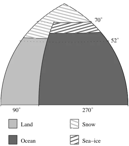
Fig. 1. Model configuration. The model consists of one hemisphere,

divided by 52◦latitude into 360◦wide, low-mid latitude and high latitude sectors. Values for global reservoirs, transports and fluxes are twice the hemispheric values. The model ocean is 270◦wide and extends from the equator to 70◦ latitude. The ocean covers 70.5% of the model surface. Low-mid latitude and high latitude ocean sectors have the area ratio 84:16. Sea ice and snow coverage are diagnosed from idealized, meridional profiles of atmospheric temperature.

1 Introduction

Earth System Models are needed as tools for understanding past global changes and for projecting future global change. The atmospheric concentration of carbon dioxide,pCO2, is a key feature of the Earth system via greenhouse radiative forcing of climate and this concentration is determined for different time scales by different Earth system components. For example, ocean circulation and biogeochemical cycling are most important forpCO2on time scales of hundreds to thousands of years whereas lithosphere outgassing and rock weathering are most important on time scales of hundreds of thousands to millions of years. Thus carbon cycle compo-nents needed in Earth System Models will depend upon time scales to be addressed in the modelling work.

On the other hand, time scales that can be addressed by Earth System Models are restricted by their complexity and spatial resolution, given available computational resources. For example, comprehensive Earth System Models of high complexity and spatial resolution built around Atmosphere-Ocean General Circulation Models can nowadays be inte-grated over thousands of years and have been extended to

include land and ocean biogeochemical cycling, important over these time scales (Cox et al., 2000; Doney et al., 2006; Schmittner et al., 2008). Only very recently have com-prehensive Earth System Models of intermediate complex-ity and spatial resolution been developed that can be inte-grated over tens of thousands of years and that have been extended to include ocean sediments, important over these longer time scales (Ridgwell and Hargreaves, 2007; Brovkin et al., 2007).

Here we describe a new, comprehensive Earth System Model of low complexity and spatial resolution called the DCESS (Danish Center for Earth System Science) model. This model includes a lithosphere module with outgassing and climate dependent-rock weathering in addition to atmo-sphere, ocean, land biosphere and ocean sediment modules. The sediment module features a new, semi-analytical treat-ment and accounts for depth- and composition-dependent porosity, oxic and anoxic remineralization, calcite dissolu-tion and burial of organic carbon and calcite. As such, this module is sufficiently flexible to deal with shallow, high pro-ductive as well as deep, low propro-ductive regions. Our model is thus suited for investigating Earth system changes on scales of years to millions of years and it can easily be integrated over these time scales.

The DCESS model has been developed in the spirit of the high-latitude exchange/interior diffusion-advection (HILDA) model in the sense that model parameters are cal-ibrated to the greatest extent possible by fitting model out-put to Earth system data (Shaffer, 1993, 1996; Shaffer and Sarmiento, 1995). As demonstrated by the applications of the HILDA model over recent years, results from a well-calibrated, low order model are useful and trustworthy within the bounds of their low spatial resolution (Gerber et al., 2004; Friedlingstein et al., 2006). Fast, low-order models like the DCESS model are also well suited for sensitivity studies and for hypothesis testing that can provide guidance for the ap-plication of more complex models.

4 2 PO ,O , DIC, ALK

100

500

1000

2000

3000 4000 5000

Depth (m)

84% 16%

PIC

s

w

PIC q

Aerobic Anoxic

BL (10 cm)

POM

POM NCM

NCM

K_vLL

K_h

K_vHL

Fig. 2. Ocean and ocean sediment configurations. Both low-mid latitude and high latitude ocean sectors are continuously-stratified with

100 m vertical resolution to maximum depths of 5500 m and each sector has a bottom topography based on real ocean depth distribution (Shaffer and Sarmiento, 1995). Model ocean circulation and mixing are indicated by the black arrows and associated circulation/mixing type labels. Model ocean biogeochemical cycling is indicated by the colored arrows (acting in both sectors but for simplicity only shown for the low-mid latitude sector) and associated matter (particulate organic (POM), biogenic carbonate (PIC) and inert mineral (NCM)). Each of the 110 model sediment segments has an area set by the real ocean depth distribution and consists of a 10 cm thick, bioturbated layer divided into 7 sublayers. Sediment biogeochemical cycling is indicated by colored arrows and associated matter. Exchange of dissolved species at the sediment-water interface is also indicated. The sedimentation rate down out of the bioturbated layer (ws)is calculated from mass conservation. See Sects. 2.3 and 2.4 and Appendix A for details.

2 Model description

The DCESS model contains atmosphere, ocean, ocean sedi-ment, land biosphere and lithosphere components. Sea ice and snow cover are diagnosed from estimated meridional profiles of atmospheric temperature. The model geome-try consists of one hemisphere, divided into two 360◦wide zones by 52◦latitude (Fig. 1). Values for global reservoirs, transports and fluxes are obtained by doubling the hemi-spheric values. The model ocean is 270◦wide and extends from the equator to 70◦latitude. In this way the ocean covers 70.5% of the Earth surface and is divided into low-mid and high latitude sectors in the proportion 84:16 as in the one hemisphere, HILDA model (Shaffer and Sarmiento, 1995). Each ocean sector is divided into 55 layers with 100 m verti-cal resolution to maximum depths of 5500 m (Fig. 2). Each of the 110 ocean layers is assigned an ocean sediment sec-tion. Ocean layer and sediment sector widths are determined from observed ocean depth distributions.

2.1 Atmosphere exchange, heat balance and ice/snow extent

We use a simple, zone mean, energy balance model for the near surface atmospheric temperature, Ta (◦C), forced by yearly-mean insolation, meridional sensible and latent heat transports and air-sea exchange. In combination with the simple sea ice and snow parameterizations, the model

in-cludes the ice/snow-albedo feedback and the insulating effect of sea-ice. Prognostic equations for meanTain the 0–52◦and 52◦–90◦zones,Tal,h, are obtained by integrating the surface energy balance over the zones. Thus,

Al,hρ0Cpbl,hdTal,h

dt = ±Fmerid−a2

Z 360

0

Z 52,90

0,52

(Ftoa−FT)cos(θ )dφdξ (1) whereAl,hare zone surface areas andρ0Cpbl,hare zone heat capacities, expressed as water equivalent capacities, whereby Cpis the specific heat capacity [4×103J (kg◦C)−1],ρ0is the reference density of water (1×103kg m−3), bl,h are thick-nesses (bl=5 m,bh=20 m, from Olsen et al., 2005),ais the Earth’s radius,θis latitude andξ is longitude. Furthermore, Fmerid is the loss (low-mid latitude) or gain (high latitude) of heat due to meridional transports across 52◦andFtoaand FT are the vertical fluxes of heat through the top of the atmo-sphere and the ocean surface. A no flux boundary condition has been applied at the equator and at the pole.

Latitudinal variations ofTa in the model are represented by a second order Legendre polynomial in sine of latitude (Wang et al., 1999),

Ta(θ )=T0+(T12)

h

3 sin2θ−1i (2)

values,Tal,h(θ ), in each hemisphere. The temperatures and temperature gradients entering Eqs. (3), (4), (5) and (8) be-low are obtained via Eq. (2).

Observations show that eddy heat fluxes in the mid-latitude atmosphere are much greater than advective heat fluxes there (Oort and Peixoto, 1983). By neglecting the ad-vective heat fluxes, Wang et al. (1999) developed suitable ex-pressions forFmeridand the associated moisture flux,Emerid, in terms ofTaand∂Ta/∂θ,

Fmerid = − h

Kt+LvKqexp

−5420T_a−1i

∂Ta∂θ

m−1

∂Ta∂θ (3)

Emerid = −Kqexp

−5420T_a−1∂Ta∂θ

m−1

∂Ta∂θ (4) whereKt is a sensible heat exchange coefficient,Kq is a la-tent heat exchange coefficient andLvis the latent heat of con-densation (2.25×109J m−3). From observations,mis found to vary with latitude (Stone and Miller, 1980) and on this ba-sis we takemto be 2.5 at 52◦_.Emerid_{enters (leaves) the high} (low-mid) latitude, ocean surface layer.

For the heat flux at the top of the atmosphere we take,

Ftoa=A+BTa−(1−α)Q (5)

where the outgoing long wave radiation is A+BTa(Budyko, 1969), whereby A and BTa are the flux at Ta=0 and the deviation from this flux, respectively. This simple formu-lation includes implicitly the radiative effects of changes in cloud cover and in atmospheric water vapor content. Green-house gas forcing is modeled by takingAto depend on de-viations of (prognostic) atmospheric partial pressures of the carbon dioxide, methane and nitrous oxide (pCO2, pCH4 andpN2O; see Sect. 2.2) from their pre-industrial (PI) val-ues such that

A=API−ACO2 −ACH4 −AN2O (6)

where expressions forACO2, ACH4andAN2Oare taken from

Myhre et al. (1998). For example, ACO2 =5.35 ln pCO2/pCO2,PI

. (7)

We take the year 1765 as our pre-industrial baseline and pCO2,PI, pCH4,PI and pN2OPI then to be 278, 0.72 and 0.27µatm, respectively, from ice core observations (Meure et al., 2006). Furthermore, α in Eq. (5) is the plane-tary albedo, equal to 0.62 for ice and snow-covered areas and to 0.3+0.08753 sin2θ−1otherwise, including the ef-fects of mean cloud cover and lower solar inclination at higher latitudes (Hartman, 1994). Finally,Qis the yearly-mean, latitude-dependent, short-wave radiation, taken to be (Q0/4)1+(Q2/2)3 sin2θ−1 whereQ0is the solar con-stant, at present 1365 W m−2_{, andQ}

2is−0.482 (Hartmann, 1994).

For air-sea heat exchange we take, from Haney (1971), FT = −Lo−KAS(Tal,hni−Tol,h) (8)

whereLo is the direct (solar) heating of the ocean surface layer, taken to be 30 and 0 W m−2 _{for the low-mid latitude} and high latitude sectors, respectively, as a good approxima-tion (Haney, 1971), KAS is a constant bulk transfer coeffi-cient, taken to be 30 W m−2 ◦C−1 but set to zero for areas covered by sea-ice, Tal,hni are mean atmospheric tempera-tures for the low-mid latitude sector and for the ice-free part of the high latitude sector, andTol,hare the zone mean, ocean surface temperatures (see below).

Finally, we take the sea ice and snow line latitudes to be located where (prescribed) atmospheric temperaturesTice andTsnoware found in the atmospheric temperature profile (Eq. 2). TiceandTsnoware taken to be−5 and 0◦C, respec-tively.

2.2 Atmosphere chemistry and air-sea gas exchange We take the atmosphere to be well mixed for gases and con-sider the partial pressures of12,13,14CO2,12,13,14CH4, N2O and O2. The prognostic equation for the partial pressure of a gasχ is taken to be

υad(p(χ ))

dt =Al_o9_Sl(χ )+Ahni₀ 9_Sh(χ )+9I(χ ) (9) where υa is the atmospheric mole volume (1.733×1020moles atm−1), Al_o is the low-mid latitude, ocean surface area, Ahni_o is the ice free part of the high latitude, ocean surface area,9l,h_S are the low-mid and high latitude, air-sea gas exchange fluxes and9I are sources or sinks within the atmosphere or net transports to or from the atmosphere via weathering, volcanism, interaction with the land biosphere and, for recent times, anthropogenic activities.

Air-sea exchange for12CO2is written 9_Sl,h=kl,h_w ηl,h_CO

2

pCO2−pCOl,h_2,w

(10) where the gas transfer velocities k_wl,h are 0.39u2 Scl,h/6600.5 whereby ul,h are the mean wind speeds at 10 m above the ocean surface and Scl,h _{are CO}

2 Schmidt numbers that depend on prognostic temperatures of the ocean surface layers (Wanninkhof, 1992), and ηl,h_CO

2

Air-sea exchange fori_CO

2withi=13 and 14 may be writ-ten

9_Sl,h=kl,h_w ηl,h_CO

2

i_α k

i_αl,h

awpiCO2−iαwal,hpCO l,h 2,wDI

i_Cl,h_/DICl,h ₍₁₁₎ where iαk are the kinetic fractionation factors (13αk=0.99912, Zhang et al., 1995), DIiCl,hand DICl,hare the prognostic total inorganic carbon concentrations in the ocean surface layers (see Sect. 2.4), i_αl,h

aw are fractionation factors due to different i_CO

2 solubilities. The coefficients i_αl,h

waare the overall fractionation factors due to fractionation in the dissociation reactions of ocean carbonate chemistry such that

i_αl,h wa =

n

[CO2]l,h+iα_HCOl,h ₃HCO−₃ l,h

+iαl,h_CO

3 h

CO−₃2il,h

/DICl,h (12)

wherei_αl,h HCO3 and

i_αl,h

CO3 are individual fractionation factors

for the species HCO−₃ and CO2₃− and values for the ocean surface layer concentrations of these species follow from the ocean carbonate chemistry calculations (see Sect. 2.4). Fractionation factors i_αl,h

aw, iα_HCOl,h ₃ and iα_COl,h₃ all depend upon ocean surface layer temperatures, taken from Zhang et al. (1995) for13C. For these fractionation factors,i_α

kand all other fractionation factors considered below, we assume that 14_{α=1−2(1−}13_α).

Air-sea exchange for O2may be written 9_Sl,h=kl,h_w η_Ol,h

2pO2−[O2]

l,h ₍₁₃₎

withk_wl,has above but with substitution for the O2Schmidt numbers that depend on prognostic temperatures of the ocean surface layers (Keeling et al., 1998). The O2solubility,ηl,h_O2, was converted from the Bunsen solubility coefficients that depend on prognostic temperatures, and to a lesser degree, on prognostic salinities of the ocean surface layers (Weiss, 1970) to model units using the ideal gas mole volume. The quantities [O2]l,h are the prognostic dissolved oxygen con-centrations in the ocean surface layers (Sect. 2.4). For sim-plicity we assume no air-sea exchange of methane species or of nitrous oxide.

The model includes the following sources/sinks of at-mospheric CO2: net exchange with the land biosphere (Sect. 2.6), oxidation of atmospheric methane (see below), volcanic input, weathering of “old” organic carbon in rocks and weathering of carbonate and silicate rocks (see Sect. 2.7). In recent times, there have been additional, anthropogenic CO2sources due to fossil fuel burning and sources/sinks due to land use change (mainly deforestation). All the above sources and sinks are also included for atmospheric13CO2. For atmospheric14CO2, the above sinks and sources are in-cluded except that there are no14CO2 sources from volca-noes, organic carbon weathering and fossil fuel burning, all

sources of old carbon. Radiocarbon is produced in the at-mosphere by cosmic ray flux and, in recent times, by atomic bomb testing. The cosmic ray source of atmospheric14CO2 may be expressed as Al+Ah

P14_C/AvgwhereP14_C is the

14_{C production rate (atoms m}−2_s−1_{)and A}

vg is the Avo-gadro number. A small amount of14C enters the land bio-sphere and decays there radioactively. The still smaller at-mospheric sink isλC14υap14CO2whereλC14is the radioac-tive decay rate for14C (3.84×10−12s−1). By far most of the 14_{C produced enters the ocean via air-sea exchange and by} far most of this decays within the ocean (Sect. 2.4). A small amount of14C from the ocean surface layer enters the ocean sediment via the rain of biogenic particles and part of this returns to the ocean after remineralization/dissolution in the sediment (see Appendix A).

Methane is produced by the land biosphere (Sect. 2.6) and, in recent centuries, by human activities. “Melting” of methane hydrate in the arctic tundra and in ocean sediments may represent yet another methane source. The main at-mospheric sink of methane is associated with reaction with OH radicals in the troposphere. Since this reaction de-pletes the concentration of these radicals, atmospheric life-times for methane grow as methane concentrations increase. We model this effect, together with the effects of associated chemical reactions in the troposphere and stratosphere, by fitting a simple model to results from a complex atmospheric chemistry model (Schmidt and Shindell, 2003). Thus, we take the atmospheric methane sink to beλCH4pCH4where

λCH4 =va(syLCH4)

−1

=[1−aM/(M+b)]va(syLCH4,PI)

−1 ₍₁₄₎

whereM≡ pCH4−pCH4,PI/pCH4,PI,syis the number of seconds in a year and LCH4, LCH4,PI are atmospheric

life-times of methane in years. We found a good fit to the re-sults of Schmidt and Shindel (loss rates in their Table 1) for a=0.96 and b=6.6. The atmospheric methane concen-tration and the total natural + anthropogenic methane sinks have been about 1.77µatm and 0.581 Gt (CH4)yr−1 in re-cent years (Table 7.6 in IPCC, 2007). These estimates lead to a present value for LCH4 of 8.4 years. Equation (14)

and the pre-industrial CH4concentration of 0.72µatm then lead to aLCH4,PI of 6.9 years, a value that implies a

pre-industrial CH4 emission of 0.286 Gt (CH4)yr−1. We esti-mate that about 0.040 Gt (CH4)yr−1of this is anthropogenic (as of year 1765). However, for simplicity, we take the entire pre-industrial emission to come from the land biosphere (see Sect. 2.6).

Nitrous oxide is produced by the land biosphere (Sect. 2.6) and, in recent centuries, by human activities. For sim-plicity, we neglect any oceanic N2O sources, consistent with our neglect of air-sea exchange of N2O. The at-mospheric sink of N2O, due mainly to photodissocia-tion in the stratosphere, is taken to be λN2OpN2O where

λN2O=va(syLN2O)

−1_{. We take L}

λN2Ois 3.66×10

4_molµatm−1_s−1_{. ForpN}

2OPI=0.27µatm, the above leads to a pre-industrial, N2O sink of 0.99×104mol s−1_.

Atmospheric sinks of O2 are associated with weathering of organic carbon in rocks and oxidation of reduced carbon emitted in lithosphere outgassing (Sect. 2.7). In the model, a long term, steady state ofpO2is achieved when these sinks balance the O2source associated with burial of organic mat-ter in ocean sediments (Sect. 2.5). This O2source leads to net, long term transport of O2from the ocean to the atmo-sphere via air-sea exchange. Additional atmospheric sinks (sources) of O2are associated with decreasing (increasing) biomass on land and, in recent times, with burning of fossil fuels.

Finally, we consider atmospheric cycling of the oxygen isotopes of water. Fractionation during evaporation enriches the low-mid latitude surface ocean and depletes low-mid lat-itude atmospheric moisture in 18O. Atmospheric moisture is further depleted via condensation upon poleward trans-port and associated cooling. Upon precipitation, this mois-ture leaves the high-latitude ocean depleted in18O. Here we use the approach described in detail in Olsen et al. (2005) to model these processes, making use of the atmospheric tem-perature at the latitude dividing the two model zones (52◦), as calculated from the meridional temperature profile (Eq. 2). A key result of these calculations is an estimate for the atmo-spheric content of18O at the dividing latitude,δ18Oa(θ=52◦) whereδ18O is defined in the conventional way relative to Standard Mean Ocean Water (SMOW).

2.3 Ocean circulation and mixing

The HILDA model serves as the point of departure for the DCESS model formulation of ocean physics and biogeo-chemical cycling. As in HILDA, four physical parameters characterize ocean circulation and mixing. For the DCESS model with continuous vertical stratification in both sectors these four parameters are 1) a transport,V, associated with high latitude sinking and the deepest, low-mid latitude up-welling, 2) constant horizontal diffusion between the zones, Kh, associated with the wind-driven circulation and deep re-circulation (Shaffer and Sarmiento, 1995), 3) strong, con-stant vertical diffusion in the high latitude zone,K_vh, asso-ciated with high latitude convection and, 4) a weak, depth-dependent, vertical diffusion in the low-mid latitude zone, K_vl(z). A discussion of real ocean physical analogues of re-lated parameters in the HILDA model is given in Shaffer and Sarmiento (1995).

The deep overturning circulation,V, equals the poleward flow in the model surface layer. The transport down out of the high latitude mixed layer, equatorward between the deep-est model layers at 5500m and upward into the low-mid lat-itude surface layer isV+Emerid, the sum of ocean surface layer and atmosphere water transports from the low-mid lat-itude to the high latlat-itude model zone (note thatVEmerid).

The water transported in the atmosphere contains no dis-solved substances. This approach leads to realistic forcing of surface layer concentration/dilution of dissolved substances (like salt and alkalinity) and avoids the use of artificial salt fluxes and the need for dealing with salinity-normalized, dis-solved substances. The depth-dependent vertical velocity for each zone,wl,h(z), is calculated from continuity using model bathymetry such that wl,h(z)=(V+Emerid)/Al,h_O (z) where Al,h_O(z)are observed low-mid and high latitude zone ocean areas as functions of ocean depth (Fig. 2).

In the low-mid latitude zone, vertical diffusion is calcu-lated as

K_vl(z)=K_v,0l hN_obsl (z)/N_obs,0l i −0.5

(15) whereK_v,0l is a vertical diffusion scale, N_obsl (z)is the ob-served mean Brunt-V¨ais¨ala frequency profile for the low-mid latitude zone andK_v,0l , N_obs,0l are corresponding values at 100 m depth.N_obsl (z)is equal to

gρ0 ∂ρl_obs(z)∂z0.5 wheregis gravity,ρ0is mean water density and the observed water density profile,ρ_obsl (z), has been calculated from ob-served mean profiles of temperature and salinity from this zone (Fig. 3a, b). TheK_vl(z)parameterization is consistent with diapycnal mixing via breaking of internal waves (Gar-gett and Holloway, 1984). We found a good fit to the results of this calculation with

K_vl(z)=K_v,0l 1+5.5{1−exp(−z/4000 m)} (16) which describes a five fold increase in the vertical diffusion from the surface to the bottom layer, similar to the Bryan and Lewis (1979) vertical diffusion profile often assumed in Ocean General Circulation Models.

With the above physics and for each of the two ocean zones, conservation of an ocean tracerϕmay be written

∂ϕ ∂t +

∂vϕ ∂y +

∂wϕ ∂z =Kh

∂2ϕ ∂y2 +

∂ ∂z

Kv ∂ϕ ∂z

+9S(ϕ)+9B(ϕ)+9I(ϕ) (17) where9S denote air-sea exchange of heat, fresh water and gases,9Bdenote exchange of dissolved substances with the ocean sediment (see also Sect. 2.5 and Appendix A) and 9I denote internal source/sink terms. For the surface lay-ers, the internal source/sink terms include biological produc-tion, river inflow of dissolved substances, and the direct solar heating (low-mid latitude only). For the ocean interior, these terms include remineralization and dissolution of biogenic matter produced in the surface layers. From the assumptions above, the meridional velocity is only defined in the surface and the deepest model layers and is set byV andV+Emerid, respectively.

(Eq. 8). Concentration/dilution of the surface layer as de-scribed above provides the forcing for ocean salinity,Sl,h(z). Ocean mean salinity is 34.72 from observations. Ocean dis-tributions of 18O content in water, δ18O_wl,h(z), are forced by sources/sinks in the mid-low/high latitude surface layers equal to±Emeridδ18Oa(θ=52◦). Ocean meanδ18Owis taken to be zero. We also calculate the distribution of the18O con-tent in biogenic carbonate,δ18Ol,hc (z), whereby for benthic carbonate deposits,

δ18Ol,h_c (z)=δ18Ol,h_w (z)+(16.5−T_wl,h(z))(4.8)−1 (18) (Bemis et al., 1998). The same relation is used for pelagic carbonate but with the use of surface layerδ18Ow andT. 2.4 Ocean biogeochemical cycling

The biogeochemical ocean tracers considered here, phos-phate (PO4), dissolved oxygen (O2), dissolved inorganic car-bon (DIC) in 12,13,14C species, and alkalinity (ALK), are all forced by net (new) production of organic matter and CaCO3shells in the lighted surface layers. In addition, O2 and DI12,13,14C are forced by air-sea exchange and PO4, DI12,13,14C and ALK are forced by river inputs to the sur-face layer and concentration/dilution of this layer by evap-oration/precipitation. In the subsurface layers, the biogeo-chemical ocean tracers are forced by remineralization of or-ganic matter and dissolution of CaCO3 shells in the water column as well as exchange with the ocean sediment. DI14C is affected by radioactive decay in all ocean layers. For sim-plicity, we have neglected explicit nitrogen cycling, i.e. phos-phate is assumed to be the basic limiting nutrient, and have assumed that all biogenic export from the surface layer is in the form of particles and that all CaCO3 is in the form of calcite.

New production of organic matter in the surface layer is parameterized in terms of phosphorus (mol P m−2s−1)as NPl,h=Al,hni_o zeu(Ll,h_f /sy)POl,h₄

n

POl,h₄ .(POl,h₄ +P1/2)

o

(19) (Maier-Reimer, 1993; Yamanaka and Tajika, 1996) where Al,hnio are the ice-free ocean surface areas,zeuis the surface layer depth (100 m), sy is the number of seconds per year, POl,h₄ are the phosphate concentrations in the surface layer, andP1/2is a half saturation constant (1µmol/m3). Ll,h_f are efficiency factors, taken to be 1 for the low-mid zone and to some lower value for the high latitude zone, as determined by model fit to ocean data (Sect. 3). This is the way that the model accounts for light and iron limitation in this zone. For simplicity, we neglect dissolved organic matter such that the rate of export of particulate organic matter (POM) down out of the surface layer is equal to new production.

Sources/sinks in the surface layer due to new pro-duction are −NPl,h for PO4, −rCPNPl,h for DI12C, (rOCP+rONP)NPl,hfor O2, andrAlkPNPl,h for ALK, where rCP, rOCP, rONP and rAlkP are (Redfield) C:P, (O2)C:P,

0 5 10 15 20 25

0 1 2 3 4 5

z (km)

T (oC)

(a)

34 34.5 35 35.5 36 36.5

0 1 2 3 4 5

z (km)

S

(b)

−250 −200 −150 −100 −50 0

0 1 2 3 4 5

z (km)

∆14 C (°/

_°°

(c)

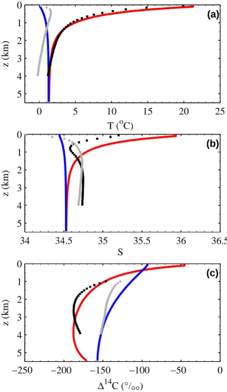
Fig. 3. Steady state, pre-industrial simulations (solid lines)

com-pared to data (dots) of mean ocean profiles of (a) temperature (T),

(b) salinity (S) and (c)114C. Low-mid latitude and high latitude

simulations are given in red and blue, respectively. Mean, data-based profiles from the low-mid and high latitude sectors are given in black and grey, respectively. These profiles have been calculated from GEOSECS data as in Shaffer and Sarmiento (1995) and Shaf-fer (1996).

with an -O2:C assimilation ratio in new production of about 1.4 (Laws, 1991). For DI13,14C, the surface layer sinks due to new production and associated isotope fractionation are

−iαl,h_Org(DIiC/DI12C)l,heurCPNPl,h (i=13 and 14) where the subscript eu refers to euphotic zone (surface layer) values. We use 13αl,h_Org=1−{17 log(CO2(aq))l,heu+3.4}/1000 (Popp et al., 1989). The empirical relationship for13αOrgassumes that (aqueous) CO2 concentrations (in units mmol m−3) mainly control this fractionation during primary production in the ocean. For a warm to cold ocean CO2(aq) range from 7 to 24 mmol m−3, this leads to a ‰ fractionation from about

−18 to−27‰ in the organic carbon produced.

The surface layer production of biogenic calcite carbon is expressed asr_CalCl,h rCPNPl,hwherer_CalCl,h are mole (“rain”) ra-tios between new production of organic and calcite12C in the surface layer. The rain ratio is parameterized as (Maier-Reimer, 1993)

r_CalCl,h =rCalC,m

h

{exp(µ(Tl,h−Tref))}

.

{1−exp(µ(Tl,h−Tref))}

i

(20) whererCalC,mis a rain ratio upper limit,µis a steepness fac-tor andTrefis a reference temperature, taken to 10◦C. Both rCalC,mandµare determined by model fit to ocean and ocean sediment data (see Sects. 3.1.3 and 3.2.1). Equation (20) yields lower rain ratios for lower temperatures as indicated by observations (Tsunogai and Noriki, 1991). Surface layer DI12Cand ALK sinks from biogenic calcite production are

−r_CalCl,h rCPNPl,h and −2r_CalCl,h rCPNPl,h, respectively. Sur-face layer DI13,14C sinks from this production and associ-ated fractionation are−iαCal(DIiC/DI12C)l,heurCalCl,h rCPNPl,h wherei=13 and 14. Here13αCalis taken to be 0.9988, corre-sponding to a fractionation of−1.2‰.

Particles are assumed to sink out of the surface layer with settling speeds high enough to neglect advection and diffu-sion of them and to take subsurface remineralization or dis-solution of them to occur instantaneously. Following Shaf-fer (1996) and further motivated by the results of ShafShaf-fer et al. (1999), we assume an exponential law for the vertical dis-tribution of remineralization of POM “carbon” and “nutri-ent” components, each with a distinct e-folding length, λN andλC, respectively. Likewise, we assume an exponential law for the dissolution of biogenic calcite particles with an e-folding length,λCal.

Thus, the vertical distributions of PO4, DI12C, O2 and ALK sources/sinks from remineralization and/or dissolution (mol m−3_s−1_{)are, respectively,}

NPl,hexp(−z/λN)/λN,

NPl,hrCP{exp(−z/λC)/λC+r_CalCl,h exp(−z/λCal)/λCal},

−NPl,h{rONPexp(−z/λN)/λN+rOCPexp(−z/λC)/λC}and NPl,h{2rCPr_CalCl,h exp(−z/λCal)/λCal−rAlkPexp(−z/λN)/λN}. (21)

The vertical distributions of DI13,14C sources from reminer-alization and dissolution are

NPl,hrCP(DIiC/DI12C)l,heu{iαOrgl,h exp(−z/λC)/λC

+iαl,h_Calr_CalCl,h exp(−z/λCal)/λCal}

(22) wherei=13 and 14. For simplicity, low-mid and high latitude values forλN,λCandλCalare assumed to be the same.

Total sources/sinks of PO4, DI12,13,14C, O2 and ALK from remineralization/dissolution at any depthzof each zone are calculated as the product of Al,h_O (z) and remineraliza-tion/dissolution fluxes atzof each zone, as calculated from Eqs. (21) and (22). The fluxes of P and 12,13,14C that fall in the form of POM and/or biogenic calcite particles on the model ocean sediment surface at any depth z of each zone are calculated as the product of dAl,h_O (z)/dz there and the difference between the particulate fluxes falling out of the ocean surface layer and the remineralization/dissolution tak-ing place down to z of each zone, as calculated by integrattak-ing Eqs. (21) and (22). Note that forλN6=λC, C:P mole ratios of POM falling on the sediment surface vary with water depth.

Model calculations of air-sea exchange of carbon diox-ide, carbon isotope fractionation during air-sea exchange and in ocean new production and dissolution of calcite in the ocean sediment require information on ocean distributions of CO2(aq) or CO2₃−. These distributions are calculated from the ocean carbonate chemistry equations, given pres-sure, model distributions of DIC, ALK, T andS and ap-propriate apparent dissociation constants for carbonic acid, boric acid and sea water as functions ofT,Sand pressure. Equations for these constants, and a relation between to-tal borate concentration andS are from Millero (1995; his Eqs. 35, 36, 52, 53 and 62) but with corrections listed in http://cdiac.ornl.gov/oceans/co2rprt.html#preseff). Alkalin-ity includes hydroxide and hydrogen ion concentration but not minor bases. This nonlinear system is solved for all car-bon species with the recursive formulation of Antoine and Morel (1995). The calculations also yield distributions of hy-drogen ion concentration (including H+bound to SO2₄−and F−)from which pH (seawater scale) is calculated. Profiles of CO2₃−saturation with respect to calcite are calculated as K_CaCO0

3(z)/{(Ca

2+₎

0S(z)/35}, where K_CaCO0 ₃ is the appar-ent dissociation constant for calcite as a function ofT,Sand pressure (Mucci, 1983) and(Ca2+₎

0 is mean ocean Ca2+, 10.57 mol m−3for present day.

2.5 Ocean sediment

thick. We do not consider dissolution and remineralization below the BL. The sediment is composed of calcite, CaCO3, non-calcite mineral, NCM, and reactive organic matter frac-tions. To a good approximation, CaCO3and NCM fractions are taken to be well mixed in the BL by bioturbation, Db, but the reactive organic matter fraction varies over the BL due to relatively rapid remineralization. We assumeDbto be con-stant over the BL and to depend on organic carbon rain rates and ambient dissolved oxygen concentrations.

For each sediment segment, NCM fluxes are prescribed based on data (see Eq. A30 in Appendix A) and calcu-lated POM and calcite rain fluxes, O2, DIC, ALK, T, S and pressure are accepted from corresponding layers of the ocean module. Calculated fluxes of PO4, O2, DIC and ALK to/from the sediment are then removed from/returned to these ocean layers. As part of these calculations, the calcite dry weight/total sediment dry weight ratio, (CaCO3)dwf, and the sedimentation velocity,ws, out of the BL are carried as prog-nostic variables. With this approach we can also deal with transient upward ws due to strong CaCO3dissolution, and the associated entrainment of buried CaCO3back up into the BL.

For each sediment segment, solutions are found for steady state profiles of reactive organic carbon (OrgC), pore-water O2 and pore-water CO2₃−. From the latter, dissolution of CaCO3in the BL is calculated and used in steady state and time dependent calculations of calcite dry weight fractions. The OrgC and O2solutions are coupled and are solved in a semi-analytical, iterative approach, given (CaCO3)dwf and ws. Explicit solutions are not sought for other species pro-duced/consumed during anoxic respiration but the influence of these species is included via boundary conditions on O2. The CaCO3and CO2₃−solutions are coupled and are solved with a semi-analytical, iterative approach (steady state) or a semi-analytical, time stepping approach (time dependent). In principle, these latter solutions also depend upon the OrgC/O2solutions via the release of CO2during remineral-ization and carbonate chemistry (Archer, 1991). Here we do not treat this effect explicitly, as it needs careful treatment for the general oxic/anoxic case we consider (see Appendix A). However, we do include this effect implicitly to some de-gree in the “water column” dissolution of CaCO3(Sect. 2.4). Steady state solutions for pore-water concentrations hold on time scales of years while steady state solutions for reactive carbon hold on times scales increasing from tens of years on continental shelves to hundreds of years in the deep ocean. 2.6 Land biosphere

We consider a land biosphere model with carbon isotope reservoirs for leaves (MG), wood (MW), litter (MD) and soil (MS). Net primary production on land, NPP, takes up CO2 from the atmosphere and depends onpCO2according to NPP=NPPPI{1+FCO2ln(pCO2/pCO2,PI)} (23)

where NPPPI is the pre-industrial level of NPP and FCO2

is a CO2 fertilization factor. Following Siegenthaler and Oeschger (1987), we take NPPPI to be 60 Gt C yr−1 and the pre-industrialMG,W,D,S reservoirs to be 100, 500, 120 and 1500 Gt C, respectively. In a comparison of 11 coupled-carbon cycle models, Friedlingstein et al. (2006) found rel-atively strong CO2fertilization in all but one of the models (their Fig. 3a). We found a good agreement to an average of their results by using Eq. (23) withFCO2 equal to 0.65, a

value adopted below. For example, this leads to an increase of NPP from 60 to 87 Gt C yr−1for apCO2doubling from 278 to 556µatm. Friedlingstein et al. (2006) found no model consensus on temperature dependence of NPP and very lit-tle dependence in five of the models of the intercompari-son. On this basis we have neglected any such dependence in Eq. (23). Following Siegenthaler and Oeschger (1987), NPP is distributed between leaves and wood in the fixed ra-tio 35:25, all leaf loss goes to litter, wood loss is divided between litter and soil in the fixed ratio 20:5, litter loss is di-vided between the atmosphere (as CO2)and the soil in the fixed ratio 45:10. Soil loss is to the atmosphere as CO2and, to a lesser extent, as CH4(see below). Organic burial on land is not considered.

Losses from all land reservoirs are taken to be propor-tional to reservoir size and, for litter and soil, to also depend upon mean atmospheric temperature according to λQ≡Q

(_T¯

a− ¯Ta,PI)/10

10 whereQ10 is a (biotic) activity increase for a 10 degree increase ofT¯a. We chose a value forQ10of 2, a typical choice in carbon-climate models (Friedlingstein et al., 2006). For temperatures at or aboveT¯a,PI, simple rela-tionships of this type approximate well the results of complex global vegetation models (Gerber et al., 2004).

Methane and nitrous oxide production occur in the soil, are proportional to the soil reservoir size and depend upon

¯

13,14_α

MλQ(λCH4,PIpCH4,PI)(

13,14_M

S/MS,PI)where13αmis the13C fractionation factor for CH4production, taken to be 0.970 corresponding to a −30‰ fractionation and a δ13C value of about−55‰ for CH4released from the soil (Quay et al., 1988).

The conservation equations for the land biosphere reser-voirs of12C are

dMG

dt=(35/60)NPP−(35/60)(NPPPI)(MG/MG,PI) (24) dMW

dt=(25/60)NPP−(25/60)(NPPPI)(MW/MW,PI)(25)

dMD

dt=(35/60)(NPPPI)(MG/MG,PI)

+(20/60)(NPPPI)(MW/MW,PI)

−(55/60)(NPPPI)λQ(MD/MD,PI) (26)

dMSdt=(5/60)(NPPPI)(MW/MW,PI)

+(10/60)(NPPPI)λQ(MD/MD,PI)

−(15/60)(NPPPI)λQ(MS/MS,PI) (27) The conservation equations for the land biosphere reservoirs of13C are

d13MGdt =13αL(p13CO2/pCO2)(35/60)NPP

−(35/60)(NPPPI)(13MG/MG,PI) (28)

d13MWdt =13αL(p13CO2/pCO2)(25/60)NPP

−(25/60)(NPPPI)(13MW/MW,PI) (29)

d13MD

dt=(35/60)(NPPPI)(13MG/MG,PI)

+(20/60)(NPPPI)(13MW/MW,PI)

−(55/60)(NPPPI)λQ(13MD/MD,P I) (30)

d13MSdt=(5/60)(NPPPI)(13MW/MW,PI)

+(10/60)(NPPPI)λQ(13MD/MD,PI)

−{(15/60)(NPPPI)−(1−13αM) λCH4,PIpCH4,PI}λQ(

13_M

S/MS,PI) (31) where13αLis the13C fractionation factor for land photosyn-thesis, taken to be 0.9819. This corresponds to a−18.1‰ fractionation, reflecting domination of C3 over C4 plant pro-ductivity, and a land biosphereδ13C value of about−25‰ (Joos and Bruno, 1998). Conservation equations for the land 14_{C reservoirs are similar to Eqs. (28–31) but with additional} radioactive sinks,−λC1414MG,W,D,S.

Inputs of12,13,14C to the atmospheric CO2pool from the land biosphere are

λQ{(45/60)(MD/MD,PI)+(15/60)(MS/MS,PI)}−

1+FCO2 ln(pCO2/pCO2,PI) (NPPPI)

(32)

and

λQ{(45/60)(13,14MD/MD,PI)+(15/60)(13,14MS/MS,PI)}− 13,14_α

L(p13,14CO2/pCO2){1+FCO2

ln(pCO2/pCO2,PI) (NPPPI)

.

With the above parameter and reservoir size choices, the pre-industrial, steady state solutions for land biosphere12,13,14_C are fully determined by prescribedpCO2,PIandpCH4,PI. 2.7 Rock weathering, volcanism and river input

Climate-dependent weathering of rocks containing phospho-rus, WP, is taken to supply dissolved phosphorus for river input,RP, such that

RP =WP =λQWP ,PI (33)

We assume that 80% and 20% of RP enter the low-mid and high latitude ocean surface layer, respectively, as shown by river runoff observations (Dai and Trenberth, 2002). For simplicity, we use the sameQ10-based, climate depen-dency for weathering as for other model components above (λQ≡Q

(T¯a− ¯Ta,PI)/10

10 )and again we take Q10 to be 2. This gives a weathering dependence on global temperature very similar that from the functione(T¯a− ¯Ta,PI)/13.7 _{used in earlier}

work (Volk, 1987). Weathering rates may also depend on other factors like continental surface area and types of ex-posed bedrock (Munhoven, 2002). These could be included into the model if needed for a specific application.

Changes in the total phosphorus content of the ocean re-flect imbalances of net inputs and outputs or

dMPdt=WP −BOrgP (34)

whereMP is the ocean phosphorus content andBOrgP is the total burial rate of phosphorus in organic matter, B_OrgPl +B_OrgPh , withB_OrgPl,h =

n−1

P

i=1

{AO{(i+1)1z}−

AO(i1z)}l,hBFl,h_OrgP(i)+AO(n1z)l,hBFl,h_OrgP(n) using the burial fluxes, BFl,h_OrgP(i), from the ocean sediment module for each of the n bottom segments with separation in depth 1zfor each of the ocean sectors. For simplicity, we assume a pre-industrial balance between total weathering and ocean burial orWP ,PI−BOrgP,PI=0. Multiplication of the above re-lationship for phosphate byrAlkP yields corresponding rela-tionships for the part of the ALK fluxes associated with or-ganic matter cycling.

The overall carbon balance of the model and the distribu-tion of carbon among the different model components are in-fluenced by climate-dependent weathering of carbonate and silicate rocks (WCalandWSil), climate-dependent weathering of rocks containing old organic carbon (WOrgC), and litho-sphere outgassing (Vol). In simple terms, silicate weathering may be described by the left to right reactions in two reaction steps

and

CaCO3+CO2+H2O⇔Ca+++2HCO−₃

Thus there is an atmosphere sink of 2 moles of CO2per mole of silicate mineral weathered. Carbonate weathering is de-scribed by the left to right reaction in the second reaction step with an atmosphere sink of 1 mole of CO2per mole of carbonate mineral weathered. Both weathering types supply HCO−₃ for river input. Then river inputs of DIC and ALK are RDIC=2(WSil+WCal)=2λQ(WSil,PI+WCal,PI) (35) and

RALK =2(WSil+WCal)−rALKPWP

=λQ{2(WSil,PI+WCal,PI)−rALKPWP ,PI}

where we assume the same 80%–20% river input partition as above and the sameQ10-based, climate dependency with Q10=2 (note that we do not consider river input of organic carbon). In the assumed, pre-industrial steady state, just enough of the biogenic carbonate falling on the sediment sur-face is buried to satisfy

WSil,PI+WCal,PI−BCal,PI=0 (36)

where total, pre-industrial calcite burial rate,BCal,PI, is cal-culated as for phosphorus burial above but with calcite burial fluxes. Likewise, pre-industrial CO2 outgassing from the ocean to the atmosphere is equal to WSil,PI+WCal,PI. An analogous relation for river input of13C can be derived in a similar way, with proper account taken for the fact that all and half of the carbon involved inWSil and WCal, respec-tively, stem from atmospheric CO2, and with a proper choice for the13C content of carbonate rock weathered duringWCal (see below).

WOrgCand Vol are the two external sources of atmospheric CO2in the model. We again adopt the sameQ10-based, cli-mate dependency andQ10=2 for weathering of old organic carbon such thatWOrgC=λQWOrgC,PI. The sources of Vol are thermal breakdown of buried carbonate and organic car-bon. Vol may either be taken constant and equal to its pre-industrial value, VolPI (see below) or may be prescribed as external forcing of the Earth system. Therefore, the total source of atmospheric CO2 from lithospheric processes is WOrgC+Vol−2WSil−WCal(all in units of moles of carbon per unit time).

Changes in total carbon content of the combined atmospheocean-land biospheocean sediment system re-flect imbalances of net inputs and outputs or

dMCdt =WCal+WOrgC+Vol−BCal−BOrgC (37) where MC is the total carbon content of this system and BOrgC is the total organic carbon burial rate, calculated as for phosphorus burial above but with organic carbon burial

fluxes. For the assumed, pre-industrial steady state, we have from Eqs. (36) and (37),

WOrgC,PI+VolPI−WSil,PI−BOrgC,PI=0 (38) With the additional assumption that silicate weathering takes place at a fixed ratio,γSil, to carbonate weathering, Eq. (36) givesWSil,PI=γSil(1+γSil)−1BCal,PIand Eq. (38) becomes WOrgC,PI+VolPI−γSil(1+γSil)−1BCal,PI−BOrgC,PI=0 (39) From a detailed study of global weathering sources, we take γSil=0.85 (Lerman et al., 2007).

An analogous, steady state equation for13C may be writ-ten as

WOrgC,PIδ13COrgC,PI+VolPIδ13CVol,PI

−γSil(1+γSil)−1BCal,PIδ13CCal,PI

−BOrgC,PIδ13COrgC,PI=0

(40)

where the δ13C are defined in the usual way relative to the PDB standard, δ13CVol,PI is taken to be −5‰ (Kump and Arthur, 1999) and δ13CCal,PI and δ13COrgC,PI are cal-culated from the steady state, pre-industrial model results (Sect. 3.2.3) as sector burial-weighted means of13C contents in organic carbon and biogenic carbonate produced in each ocean sector. Thus,δ13CCal,PI=(B_Cal,PIl δ13C

l Cal,PI

+B_Cal,PIh δ13Ch_Cal,PI)(B_Cal,PIl +B_P,PIh )−1and δ13COrgC,PI=(B_OrgC,PIl δ13C

l

OrgC,PI+BOrgC,PIh δ13C h OrgC,PI) (B_OrgC,PIl +B_OrgC,PIh )−1. For simplicity, we have assumed that the13C content of old and new organic matter are the same in this steady state. We can now solve forWOrgC,PIand VolPIusing Eqs. (39) and (40):

VolPI=γSil(1+γSil)−1(δ13CCal,PI−δ13COrgC,PI)

(δ13CVol,PI−δ13COrgC,PI)−1BCal,PI, (41)

WOrgC,PI=BOrgC,PI−γSil(1+γSil)−1

{(δ13CCal,PI−δ13COrgC,PI)

(δ13CVol,PI−δ13COrgC,PI)−1−1}BCal,PI (42) Changes in total oxygen content of the atmosphere and ocean reflect imbalances of net inputs and outputs whereby

dMOdt=rOC,LdMLdt+rONP(BP −WP)+ (rOCP/rCP){BOrgC−WOrgC−(δ13CCal−δ13CVol) (δ13CCal−δ13COrgC)−1Vol}

(43)

For the assumed, pre-industrial steady state, Eq. (43) be-comes

(rOCP/rCP){BOrgC,PI−WOrgC;PI−(13δCal,PI−13δVol,PI) (13δCal,PI−13δOrgC,PI)−1VolPI}

+rONP(BP,PI−WP,PI)=0

(44)

3 Model solution, calibration and validation

3.1 Pre-industrial steady state solution for the atmosphere and ocean

3.1.1 Solution procedure

Ocean tracer equations are discretized on a grid defined by the two meridional zones, with vertically-decreasing hor-izontal extents as set by observed ocean topography, and by constant vertical resolution of 100 m. Each of these 2×55 ocean boxes is associated with an ocean sediment seg-ment with horizontal extent set by the observed topography. Model tracer boundary conditions account for the two-way exchange of heat and freshwater between the atmosphere and the ocean as well as the two-way exchange of gases between the atmosphere and the ocean, the land biosphere and the lithosphere. Other tracer boundary conditions account for particulate matter fluxes from the ocean to the ocean sed-iment, two-way exchange of dissolved substances between the ocean and the ocean sediment, and fluxes of dissolved and particulate matter from the lithosphere to the ocean. Prog-nostic equations for the atmosphere (including snow and sea ice cover), the land biosphere, the lithosphere and the ocean are solved simultaneously using a fourth order Runge Kutta algorithm with a two week time step. Prognostic equations for the ocean sediment are solved by simple time stepping with a one year time step. The complete, coupled model was written in Matlab and runs at a speed of about 10 kyr per hour on a contemporary PC.

3.1.2 Calibration procedure

We calibrated the parameters of the DCESS model by “trial and error” in four steps. In the first calibration step we considered the atmosphere module only with atmospheric pCH4 and pN2O set at pre-industrial values of 0.72µatm and 0.27µatm, respectively, and with atmosphericpCO2set at its pre-industrial value of 278µatm or at twice that value, 556µatm (Etheridge et al., 1998a, b; Meure et al., 2006). We adjusted the four free parameters of this module (Table 1) to give a global mean atmospheric temperature of 15◦C and a climate sensitivity of 3◦C per doubling of atmosphericpCO2 and poleward heat and water vapor transports in the atmo-sphere across the sector boundary consistent with observa-tions (Trenberth and Caron, 2001; Dai and Trenberth, 2002). In the second calibration step, we considered the ocean and land biosphere modules coupled to the

preliminarily-calibrated, atmosphere module, with pre-industrial atmo-spheric δ13C of −6.4‰, observed atmospheric pO2 of 0.2095 atm and observed ocean mean PO4, DIC and ALK of 2.12×10−3, 2.32 and 2.44 mol m−3(Francey, 1999; Keel-ing et al., 1998; Shaffer, 1993, 1996). Atmospheric14C pro-duction was adjusted to maintain atmospheric114C at 0‰. In this step we assumed that all biogenic particles falling to the ocean bottom remineralize completely there. We then made initial guesses for the values of the 10 free parame-ters of the ocean module of which 4 are physical and 6 are biogeochemical (Table 1). These guesses were based in part on results from the HILDA model calibration (Shaffer, 1993, 1996; Shaffer and Sarmiento, 1995) and in part on literature values (Maier-Reimer, 1993). Note that values of all param-eters in the land biosphere model were determined a priori.

The resulting atmosphere-ocean-land biosphere model was spun up from uniform atmosphere and ocean tracer dis-tributions to a steady state solution after about 10 000 model years and results were compared with atmosphere and ocean data. Then parameter values were adjusted by expertise-guided “trial and error” to obtain steady state solutions that better satisfied a global mean atmospheric temperature of 15◦C, a climate sensitivity of 3◦C per doubling of atmo-spheric pCO2, an atmospheric pCO2 value of 278µatm, observed poleward heat and water vapor transports across the sector boundary (52◦ latitude) and observed ocean dis-tributions of T,14C, PO4, O2, DIC and ALK (Shaffer, 1993, 1996; Shaffer and Sarmiento, 1995). Note that atmospheric transport parameters were reduced in this step to obtain good model fit in the presence of meridional heat transports in the ocean.

In the third calibration step, we coupled our ocean sedi-ment module to the model of the second step. In the resulting closed system, a tracer flux was added in appropriate form to the ocean surface layer of a sector at a rate equal to the total burial rate of that tracer in that sector from the sediment mod-ule. We then made initial guesses for the values of the 4 free parameters of the sediment module (Table 1), based on pub-lished results (Archer et al., 1998, 2002). With these values and parameter values from the second calibration step, we solved for a new, pre-industrial steady state, taking advan-tage of the fast, steady state mode of the sediment module (see Appendix A). Then all model parameter values were ad-justed by expertise-guided “trial and error” to obtain steady state solutions that better satisfied the data-based constraints of the second calibration step in addition to observed calcite and organic carbon distributions and inventories in the ocean sediment (Hedges and Keil, 1995; Archer, 1996a).

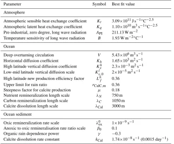
Table 1. Standard case values for tunable model parameters.

Parameter Symbol Best fit value

Atmosphere

Atmospheric sensible heat exchange coefficient Kt 3.09×1011J s−1◦C−2.5 Atmospheric latent heat exchange coefficient Kq 1.10×1010m3s−1◦C−2.5 Pre-industrial, zero degree, long wave radiation API 211.13 W m−2

Temperature sensitivity of long wave radiation B 1.93 W m−2◦C−1 Ocean

Deep overturning circulation V 5.43×106m3s−1 Horizontal diffusion coefficient Kh 1.65×103m2s−1 High latitude vertical diffusion coefficient K_vh 2.3×10−3m2s−1 Low-mid latitude vertical diffusion scale K_v,0l 2×10−5m2s−1 High latitude new production efficiency factor Lh_f 0.36

Upper limit for rain ratio rCalC,m 0.36 Steepness factor for calcite production µ 0.18 Nutrient remineralization length scale λN 750 m Carbon remineralization length scale λC 1050 m Calcite dissolution length scale λCal 3000 m

Ocean sediment

Oxic remineralization rate scale λ0_ox 1×10−9s−1 Anoxic to oxic remineralisation rate ratio scale β0 0.1

Organic rain dependence power γ −0.3

Calcite dissolution rate constant kCal 1.74×10−8s−1(0.0015 day−1)

pre-anthropogenic steady state for P and 12,13C. We then made slight final “trial and error” adjustments of model pa-rameters values and of ocean mean PO4, DIC and ALK until the model steady state results again broadly satis-fied the data-based constraints of the third calibration step. For this final calibration, atmospheric production of14C is 1.8752×104atom m−2_s−1 _{and the ocean mean PO}

4, DIC and ALK are 2.089×10−3_{, 2.318 and 2.434 mol m}−3_, respec-tively, that may be compared with the observed ocean inven-tories above.

3.1.3 Ocean tracer and biological production results Our tuned parameter values for this pre-industrial, steady state calibration are listed in Table 1. The sea ice and snow lines for this solution are found at 63.5 and 55.8◦ _latitude, respectively. The total poleward heat transport across 52◦ latitude in this steady state is 5.0 PW, with ocean and at-mosphere contributions of 0.7 PW and 4.3 PW, respectively. Poleward water vapor transport in the atmosphere there is 0.36 Sv (1 Sv=106m3s−1). All these transport estimates agree well with recent data and reanalysis based estimates (Trenberth and Caron, 2001; Dai and Trenberth, 2002). The atmospheric heat transport is divided between sensible and latent heat as 3.44 PW and 0.80 PW, respectively. The ocean

heat transport consists of 0.23 PW in the deep upwelling cir-culation,V, and 0.50 PW in the wind-driven circulation and deep recirculation associated withKh.

Equation (16) and the best fit estimate for the diffu-sion scale lead to an increase in vertical diffudiffu-sion from 2×10−5m2s−1to 10.2×10−5m2s−1down through the low-mid latitude ocean. This agrees with observations of weak background mixing combined with bottom intensified mix-ing near rough topography (Ledwell et al., 1998; Polzin et al., 1997). However, our simple model does not capture the vertical component of ocean isopycnal mixing, an important component of upper ocean vertical exchange of tracers like 14_{C and O}

2(Siegenthaler and Joos, 1992). Our simultaneous tuning to fit to such tracers and to temperature (which largely defines isopycnals and is therefore not mixed along them) is a tradeoff tending to overestimate the effective vertical change of heat but to underestimate the effective vertical ex-change of the other tracers. But this is a useful tradeoff since it helps limit the number of model free parameters while still allowing good model agreement with observations.

0

0.5

1

1.5

2

2.5

3

0

1

2

3

4

5

z (km)

P (mmol m

)

(

a

)

0.1

0.15

0.2

0.25

0.3

0.35

0.4

0

1

2

3

4

5

z (km)

O

2

(mol m

)

(

b

)

1.9

2

2.1

2.2

2.3

2.4

2.5

0

1

2

3

4

5

z (km)

DIC (mol m

)

(

c

)

2.1

2.2

2.3

2.4

2.5

2.6

2.7

0

1

2

3

4

5

z (km)

Alk (eq m

)

(

d

)

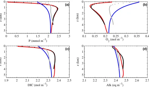
Fig. 4. Steady state, pre-industrial simulations (solid lines) compared to data (dots) of mean ocean profiles of (a) phosphate (P), (b) dissolved

oxygen (O2), (c) dissolved inorganic carbon (DIC) and (d) alkalinity (ALK). Low-mid latitude and high latitude simulations are given in red and blue, respectively. Mean, data-based profiles from the low-mid and high latitude sectors are given in black and grey, respectively. These profiles have been calculated from GEOSECS data as in Shaffer and Sarmiento (1995) and Shaffer (1996).

only ocean data from below 1000 m have been used as shal-lower depths are strongly affected by atomic bomb14C. With best fit parameters, the model achieves generally good fits to T and114C data. The high latitude temperature observations reflect deep water formation in geographically restricted sites not resolvable in our simple model. Model114C minimum for the low-mid latitude sector lies about 1 km deeper than in the observations and model114C values for the high lati-tude sector are a little high in the depth range 1000–2500 m. Model fit to the salinity data is not very good since salin-ity distributions in the real ocean are strongly controlled by vertically-structured, advective processes not captured in our simple model. In particular, the salinity minimum in the data at about 800 m depth reflects low saline, intermediate waters formed in the 50–60◦ _{latitude band. The presence of these} waters also helps maintain low-mid latitude, surface layer salinity relatively low.

Model ocean profiles of PO4, O2, DIC and ALK are shown in Fig. 4, together with data-based, mean sector profiles of these tracers. With best fit parameters, the model achieves good fits to PO4, O2, and DIC data in the low-mid latitude sector. High latitude sector differences in vertical structure between data and model simulations reflect geographically

restricted deep water formation and vertically-structured, ad-vective processes, as mentioned above. As in Shaffer (1996), simultaneous tuning to fit PO4 and O2 data reveal slower remineralization of the “carbon” component compared to the “nutrient” component of POM, as reflected by λC>λN in Table 1. This important property of POM remineralization in the ocean was also documented in an in-depth analysis of ocean tracer data (Shaffer et al., 1999). Model fit to ocean ALK data in the low-mid latitude sector is less im-pressive but still serves to help constrain the global biogenic calcite production and the calcite dissolution length scale, λCal. As for salinity, the relative model misfit to low-mid latitude ALK data can be traced to a relatively strong in-fluence of vertically-structured, advective processes in the ocean. Model ocean profiles of CO2₃−are shown in Fig. 7a. The crossing point for CO2₃− and the CO2₃− saturation pro-files is the calcite saturation depth (CSD). Model CSD’s are 2928 m and 3186 m for the low-mid and high latitude zones, respectively. The model CSD’s are 400–500 m shallower than the data-based estimates (Fig. 7a). This can be traced back to the ALK profile misfits discussed above.

−2 −1 0 1 2 3 4 0

1 2 3 4 5

z (km)

δ18 O (°/

_°°

(a)

0 0.5 1 1.5 2 2.5 3

0 1 2 3 4 5

z (km)

δ13 C (°/

_°°

(b)

Fig. 5. Steady state, pre-industrial simulations (solid lines)

com-pared to data (dots) of mean ocean profiles of (a) δ18Ow and (b)δ13C. Low-mid latitude and high latitude simulations are given in red and blue, respectively. Mean, data-based profiles from the low-mid and high latitude sectors are given in black and grey, re-spectively. These profiles have been calculated from GEOSECS data as in Shaffer and Sarmiento (1995) and Shaffer (1996). Also shown are (a) simulated biogenic calciteδ18O (dashed lines), cal-culated from simulated oceanT and δ18Ow using Eq. (18) and (b) simulatedδ13C (dashed lines) for an alternative temperature-dependent fractionation (see Sect. 3.1.3). Note that ocean uptake of fossil fuel CO₂has reduced near surfaceδ13C values by about 0.5‰ from pre-industrial levels (Sonnerup et al., 1999).

and high latitude sectors, respectively. This global new pro-duction estimate is somewhat higher than the 4.6 Gt C yr−1 from Shaffer (1996) but still only about half as large as more recent estimates (cf. Falkowski et al., 2003). The tradeoff in tuning of vertical exchanges discussed above helps ex-plain our relatively low result. New production in the tuned model is strongly constrained by high latitude surface layer PO4and ocean interior PO4and O2data. This leads to the relatively low value of 0.36 for the high latitude new produc-tion efficiency factor,Lh_f, indicative of strong light and/or iron limitation in this region. Global biogenic calcite pro-duction in our solution is 0.97 Gt C yr−1, thereof 0.83 and 0.14 Gt C yr−1in the low-mid and high latitude sectors, re-spectively. This global estimate lies well within the range 0.5–1.6 Gt C yr−1 of other such estimates (Berelson et al., 2007). Our model topography and calcite dissolution length

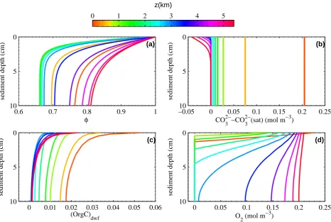
0 0.2 0.4 0.6 0.8 1

0 1 2 3 4 5

z (km)

(CaCO 3)dwf

(a)

0 0.05 0.1 0.15 0.2

0

5

10

sediment depth (cm)

CO 3 2−

& CO

2 (mol m −3

)

(b)

2.25 2.3 2.35 2.4

0

5

10

(c)

sediment depth (cm)

DIC & HCO 3 −

(mol m−3)

Fig. 6. Steady state, pre-industrial, low-mid latitude simulations

0 0.05 0.1 0.15 0.2 0.25 0.3 0

1 2 3 4 5

z (km)

CO 3 2−

& CO 3 2−

(sat) (mol m−3)

(a)

0 0.2 0.4 0.6 0.8 1

0 1 2 3 4 5

z (km)

(CaCO 3)dwf

(b)

0 0.05 0.1 0.15 0.2

0 1 2 3 4 5

z (km)

(OrgC) dwf

(c)

0 5 10 15 20 25

0 1 2 3 4 5

z (km)

w

s (cm kyr −1

)

(d)

Fig. 7. Steady state, pre-industrial simulations of distributions over water depth of (a) water column carbonate ion (CO2₃−, solid lines)

and carbonate ion saturation with calcite (dashed lines), (b) calcite dry weight fraction ((CaCO₃)dwf)exported at the base of the sediment bioturbated layer (BL, solid lines) and (CaCO3)dwf of material falling on the surface of the BL (dashed lines), (c) organic carbon dry weight fraction ((OrgC)dwf) exported at the base of the BL (solid lines) and (OrgC)dwf of material falling on the surface of the BL (dashed lines) and (d) sedimentation velocity (ws)at the base of the BL. Low-mid latitude and high latitude simulations are given in red and blue, respectively. Also shown in (a) are the low-mid and high latitude, CO2₃−profiles calculated from mean, data-based DIC and ALK profiles shown in Fig. 4 (black and grey dots, respectively). Organic matter dry weight fractions are equal to organic carbon dry weight fractions multiplied by 2.7. The sum of calcite, non-calcite mineral and organic matter dry weight fractions is equal to 1.

scale (Table 1) imply that 64% of this calcite production dis-solves in the water column; the rest falls on the sediment surface. Model calcite production is constrained strongly by ALK data but also by ocean sediment data (Sect. 3.2.1). This has led to a rather high value of 0.36 forrCalC,m, the rain ratio upper limit parameter and a rather strong temperature depen-dency of the rain ratio, as expressed by the value of 0.18 for µ. Still, the above low-mid latitude results lead to calcite carbon to organic carbon flux ratios of 0.6, 1.1 and 2.0 at 1000, 2000 and 3000 m depths, respectively, in good agree-ment with ocean sediagree-ment trap results reviewed by Berelson et al. (2007).

3.1.4 Ocean isotope results

Model ocean profiles ofδ18Owandδ13C are shown in Fig. 5, together with mean, data-based sector profiles. Atmospheric processes coupled to evaporation/precipitation forceδ18Ow. Therefore, the distribution of this tracer (Fig. 5a, solid lines) mirrors that of salinity, as can be seen by comparing model

and the data based profiles (Figs. 3b and 5a). Our treatment of δ18Ow yields correct δ18Ow:S ratios (see also Olsen et al., 2005) but significant model-data disagreements arise for δ18Ow, as for salinity. Figure 5a also shows model profiles of δ18O in biogenic carbonate,δ18Oc, calculated using Eq. (18) and model solution forT andδ18Ow.

our model fit to ocean 114C data. Excessive air-sea ex-change fractionation at low temperatures is another possible explanation. To illustrate this, we altered the formulation of the Zhang et al. (1995) temperature-dependent, fractionation factor13αHCO3, such as to yield the same value at 25

◦_{C as} the original13αHCO3but with the weaker, temperature

depen-dency slope of13αCO3. The results with the altered

13_α HCO3

show much better agreement with data, including higher sur-face layer values at low-mid latitudes than at high latitudes (Fig. 5b). We note that the Zhang et al. (1995) results are not based on any measurements at temperatures below 5◦C but we have no other reason to doubt these results. A simula-tion with a 50% increase in fracsimula-tionasimula-tion during new produc-tion also yields a considerably better model agreement with ocean meanδ13C. However, our results from such a simula-tion overestimate observed surface layer values and are not consistent with observedδ13C in ocean particulate organic matter (Hofmann et al., 2000).

3.2 Pre industrial, steady state solution for the ocean sedi-ment and the lithosphere

3.2.1 Sediment inventories

Values for the oxic remineralization rate scale, λ0_ox, the anoxic-oxic remineralization rate ratio, β0, and the organic rain dependence power,γ, have been chosen to yield model results that satisfy two conditions, given rain rates from the ocean model and the prescribed rain of non-calcite minerals. The conditions are 1) the ocean mean burial fraction for or-ganic matter falling on the sediment surface should be about 0.1 and, 2) the organic matter burial at depths of 1000 m or less should be a fraction of 0.8–0.9 of total ocean organic matter burial (Hedges and Keil, 1995). From our tuning of these parameters (Table 1), the pre-industrial, steady state values for these two fractions are 0.093 and 0.897, respec-tively. Burial fractions for the low-mid and high latitude sec-tors are 0.090 and 0.094 and the total organic carbon burial rate,BOrgC,PI, is 0.073 Gt C yr−1. Model global inventories of erodible and bioturbated layer organic carbon are 130 and 92 Gt C. The best fit value forλ0_ox agrees with sediment ob-servations for moderate organic carbon rain rates (Emerson, 1985). The best fit values forβ0andγlead to much reduced remineralization rates in the sediment under anoxic condi-tions, as indicated by data (Archer et al., 2002). As an illus-tration of model sensitivity to anoxic remineralization rate, ocean mean burial fractions are 0.316 and 0.004 when this rate is set to 0 and to the oxic rate.

The value for the calcite dissolution rate constant, kCal, in Table 1 was chosen to approximate a global inventory of erodible calcite in ocean sediments of about 1600 Gt C (Archer, 1996a) and sublysocline transition layer thicknesses around 1500–2000 m, given biogenic rain rates from the ocean model and the prescribed rain of non-calcite miner-als on the ocean surface. The best fit value forkCalis in the

range for which Archer et al. (1998) found good agreement among model results based on linear and non-linear kinet-ics for calcite dissolution. With this value, model global in-ventories of erodible and bioturbated layer calcite are 1603 and 1010 Gt C. The model mean calcite dry weight fraction (dwf) is 0.360, close to a data-based estimate of 0.34 (Archer 1996a). The calcite burial rate for the pre-industrial, steady state solution,BCal,PI, is 0.20 Gt C yr−1of which 0.13 Gt C yr−1takes place at water depths greater than 1000 m. Results above give an overall calcite-C to organic carbon-C burial ra-tio of less than 3 while the corresponding overall sediment inventory ratio is greater than 10. This contrast is explained by the fact that most of the sediment organic carbon is found at shallow depths where the sedimentation velocity is much greater than deeper down.

To test the influence of porosity formulations on our re-sults, we recalculated steady state, sediment calcite carbon and organic carbon inventories using the Zeebe and Zachos (2007) function for the limiting porosity at depth,φmin, to-gether with the Archer (1996a) function for porosity change across the bioturbated sediment layer (see Sect. A1 of Ap-pendix A). This is the same approach as was used by Ridg-well (2007). With this formulation, model global inventories of erodible and bioturbated layer organic carbon are 159 and 80 Gt C and model global inventories of erodible and bio-turbated layer calcite are 1659 and 754 Gt C. These results are similar to those reported above from our standard poros-ity formulation but show slightly lower bioturbated layer in-ventories. The lower inventory for bioturbated layer calcite agrees somewhat better with a data-based estimate of about 800 Gt C (Archer, 1996a). We also recalculated these inven-tories for assumed constant sediment porosity and obtained quite different results with considerably lower calcite inven-tories for example. These findings underline the importance of using an appropriate depth- and composition-dependent porosity formulation in an ocean sediment module.

3.2.2 Bioturbated sediment layer distributions