www.geosci-model-dev.net/9/4381/2016/ doi:10.5194/gmd-9-4381-2016
© Author(s) 2016. CC Attribution 3.0 License.
Evaluating lossy data compression on climate simulation data within
a large ensemble
Allison H. Baker1, Dorit M. Hammerling1, Sheri A. Mickelson1, Haiying Xu1, Martin B. Stolpe2, Phillipe Naveau3, Ben Sanderson1, Imme Ebert-Uphoff4, Savini Samarasinghe4, Francesco De Simone5, Francesco Carbone5, Christian N. Gencarelli5, John M. Dennis1, Jennifer E. Kay6, and Peter Lindstrom7
1The National Center for Atmospheric Research, Boulder, CO, USA
2Institute for Atmospheric and Climate Science, ETH Zurich, Zurich, Switzerland 3Laboratoire des Sciences du Climat et l’Environnement, Gif-sur-Yvette, France
4Department of Electrical and Computer Engineering, Colorado State University, Fort Collins, CO, USA 5CNR-Institute of Atmospheric Pollution Research, Division of Rende, UNICAL-Polifunzionale, Rende, Italy 6Department of Oceanic and Atmospheric Sciences, University of Colorado, Boulder, CO, USA
7Center for Applied Scientific Computing, Lawrence Livermore National Laboratory, Livermore, CA, USA Correspondence to:Allison H. Baker ([email protected])
Received: 8 June 2016 – Published in Geosci. Model Dev. Discuss.: 25 July 2016 Revised: 21 October 2016 – Accepted: 7 November 2016 – Published: 7 December 2016
Abstract. High-resolution Earth system model simulations generate enormous data volumes, and retaining the data from these simulations often strains institutional storage resources. Further, these exceedingly large storage requirements nega-tively impact science objectives, for example, by forcing re-ductions in data output frequency, simulation length, or en-semble size. To lessen data volumes from the Community Earth System Model (CESM), we advocate the use of lossy data compression techniques. While lossy data compression does not exactly preserve the original data (as lossless com-pression does), lossy techniques have an advantage in terms of smaller storage requirements. To preserve the integrity of the scientific simulation data, the effects of lossy data com-pression on the original data should, at a minimum, not be statistically distinguishable from the natural variability of the climate system, and previous preliminary work with data from CESM has shown this goal to be attainable. However, to ultimately convince climate scientists that it is acceptable to use lossy data compression, we provide climate scientists with access to publicly available climate data that have un-dergone lossy data compression. In particular, we report on the results of a lossy data compression experiment with out-put from the CESM Large Ensemble (CESM-LE) Commu-nity Project, in which we challenge climate scientists to ex-amine features of the data relevant to their interests, and
at-tempt to identify which of the ensemble members have been compressed and reconstructed. We find that while detecting distinguishing features is certainly possible, the compression effects noticeable in these features are often unimportant or disappear in post-processing analyses. In addition, we per-form several analyses that directly compare the original data to the reconstructed data to investigate the preservation, or lack thereof, of specific features critical to climate science. Overall, we conclude that applying lossy data compression to climate simulation data is both advantageous in terms of data reduction and generally acceptable in terms of effects on scientific results.
1 Introduction
proces-sor speeds over the last 25 years, the cost of storing huge data volumes is becoming increasingly burdensome and consum-ing larger and unsustainable percentages of computconsum-ing center budgets (e.g., Kunkel et al., 2014).
The Community Earth System Model (CESM) is a popu-lar and fully coupled climate simulation code (Hurrell et al., 2013), whose development is led by the National Center for Atmospheric Research (NCAR). The CESM regularly produces large datasets resulting from high-resolution runs and/or long timescales that strain NCAR storage resources. For example, to participate in the Coupled Model Compari-son Project Phase 5 (CMIP5, 2013) that led to the Intergov-ernmental Panel on Climate Change (IPCC, 2016) Assess-ment Report 5 (AR5) (IPCC, 2013), CESM produced nearly 2.5 PB of raw output data that were post-processed to obtain the 170 TB of data submitted to CMIP5 (Paul et al., 2015). Current estimates of the raw data requirements for CESM for the upcoming CMIP6 project (Meehl et al., 2014) are in excess of 10 PB (Paul et al., 2015). A second example of a data-intensive CESM project is the CESM-Large Ensemble (LE) project (Kay et al., 2015), a large ensemble climate sim-ulation study. The CESM-LE project is a publicly available collection of 180-year climate simulations at approximately 1◦ horizontal resolution for studying internal climate vari-ability. Storage constraints influenced the frequency of data output and necessitated the deletion of the raw monthly out-put files. In particular, the initial 30 ensemble member sim-ulations generated over 300 TB of raw data, and less than 200 TB of processed and raw data combined could be re-tained due to disk storage constraints. For large climate mod-eling projects such as CMIP and CESM-LE, reducing data volumes via data compression would mitigate the data vol-ume challenges by enabling more (or longer) simulations to be retained, and hence allow for more comprehensive scien-tific investigations.
The impact of data compression on climate simulation data was addressed in Baker et al. (2014). In Baker et al. (2014), quality metrics were proposed to evaluate whether errors in the reconstructed CESM data (data that had under-gone compression) were smaller than the natural variability in the data induced by the climate model system. The results of the preliminary study indicated that a compression rate of 5 : 1 was possible without statistically significant changes to the simulation data. While encouraging, our ultimate goal is to demonstrate that the effect of compression on the climate simulation can be viewed similarly to the effect of a small perturbation in initial conditions or running the exact same simulation on a different machine. While such minor mod-ifications lead to data that are not bit-for-bit (BFB) identi-cal, such modifications should not result in an altered climate (Baker et al., 2015). With compression in particular, we must also ensure that nothing systematic (i.e., over-smoothing) has been introduced. Therefore, to build confidence in data com-pression techniques and promote acceptance in the climate community, our aim in this work is to investigate whether
applying lossy compression impacts science results or con-clusions from a large and publicly available CESM dataset.
To this end, we provided climate scientists with access to climate data via the CESM-LE project (Kay et al., 2015). We contributed three additional ensemble members to the CESM-LE project and compressed and reconstructed an un-specified subset of the additional three members. To deter-mine whether the effects of compression could be detected in the CESM-LE data, we then enlisted several scientists to attempt to identify which of the new members had under-gone lossy compression by using an analysis technique of their choosing (i.e., we did not specify what analysis tech-nique each should use). In addition, we provided a different group of scientists with both the original and reconstructed datasets and asked them to directly compare features par-ticular to their interests (again, we did not specify how this analysis should be done) and determine whether the effects of compressing and reconstructing the data impacted cli-mate features of interest. Indeed, a significant contribution of our work was enabling scientists to evaluate the effects of compression on any features of the data themselves with their own analysis tools (rather than relying solely on sim-ple error metrics typically used in compression studies). Note that while the three additional CESM-LE ensemble members were generated at NCAR, the scientists participating in the ensemble data evaluations were from both NCAR and exter-nal institutions. The author list for this paper reflects both those who conducted the study as well as those who par-ticipated in the lossy data evaluations (and whose work is detailed in this paper). For simplicity, the term “we” in this paper can indicate any subset of the author list, and in Ap-pendix A we detail which authors conducted each of the data evaluations described in this work.
2 Background
In this section, we further discuss lossy data compression. We then provide additional details on the CESM-LE project datasets.
2.1 Data compression
Compression techniques are classified as either lossless or lossy. Consider a dataset X that undergoes compression, resulting in the compressed dataset C (X⇒C). When the data arereconstructed, thenC⇒Xe. If the compression tech-nique is lossless, then the original data are exactly preserved:
X =Xe. Note that the commonly usedgzipcompression util-ity is a lossless method. If, on the other hand, the compres-sion technique is lossy, thenX≈Xe; the data are not exactly the same (e.g., Sayood, 2012). Lossy compression methods generally give the user some control over the information loss via parameters that either control the compression rate, precision, or absolute or relative error bounds. The effective-ness of compression is generally measured by a compression ratio (CR), which is the ratio of the size of the compressed file to that of the original file (cf. Iverson et al., 2012): CR(F )= filesize(C)
filesize(X). (1)
While lossless methods are often viewed as “safer” for sci-entific data, it is well known that lossless data compression of floating-point simulation data is difficult and often yields lit-tle benefit (e.g., Lindstrom and Isenburg, 2006; Bicer et al., 2013; Lakshminarasimhan et al., 2011). The reason for the relative ineffectiveness of lossless methods on scientific data (in contrast to image or audio data, for example) is that trail-ing digits of the fixed-precision floattrail-ing-point output data are often essentially random, depending on the data type and the number of physically significant digits. Random numbers are a liability for compression, thus giving lossy methods a sig-nificant advantage. Many recent efforts have focused on ef-fectively applying or adapting lossy techniques for scientific datasets (e.g., Lakshminarasimhan et al., 2011; Iverson et al., 2012; Laney et al., 2013; Gomez and Cappello, 2013; Lind-strom, 2014). In the climate modeling community in particu-lar, lossy data compression has been the subject of a number of recent studies (e.g., Woodring et al., 2011; Hübbe et al., 2013; Bicer et al., 2013; Baker et al., 2014; Kuhn et al., 2016; Silver and Zender, 2016; Zender, 2016), though we are not aware of comparable efforts on evaluating the effects on the scientific validity of the climate data and results.
A major obstacle inhibiting the adoption of lossy com-pression by many scientific communities is not technical, but rather psychological in nature. For example, scientists, who analyze the climate simulation data, are often (under-standably) reluctant to lose bits of data in order to achieve smaller data volumes (hence the continued interest in loss-less approaches, such as recent work in Huang et al., 2016,
and Liu et al., 2014). In remarkable contrast, meteorologi-cal communities widely use and trust the World Meteoro-logical Organization (WMO) accepted GRIB2 (Day et al., 2007) file format, which encodes data in a lossy manner. It should be noted, however, that difficulties can arise from GRIB2’s lossy encoding process, particularly with new vari-ables with large dynamic ranges or until official GRIB2 spec-ification tables are released for new model output (see, e.g., GFAS, 2015). While the preliminary work in Baker et al. (2014) indicated that GRIB2 was not as effective as other compression methods on CESM data, a more extensive in-vestigation of GRIB2 with climate data should be done in light of the new techniques in Baker et al. (2015) and this paper before definitive conclusions are drawn. Nevertheless, the contrast is notable between the meteorological commu-nity’s widespread use and acceptance of GRIB2 and the cli-mate community’s apparent reluctance to adopt lossy meth-ods, even when proven to be safe, flexible and more effective. In this context, when applying lossy compression to scien-tific datasets, determining appropriate levels of precision or error, which result in only a negligible loss of information, is critical to acceptance.
(Com-munity Atmosphere Model version 5). Historical forcing is used for the period 1920–2005 and RCP8.5 radiative forcing (i.e., forcing that reflects near-past and future climate change; e.g., Lamarque et al., 2011) thereafter. Ensemble spread is generated using small round-off level differences in the ini-tial atmospheric temperature field. Comprehensive details on the experimental setup can be found in Kay et al. (2015).
CESM outputs raw data in NetCDF-formatted time-slice files, referred to as “history” files, for post-processing anal-ysis. Sample rates (daily, monthly, etc.) are determined for each variable by default, depending on the grid resolution, though a user can specify a custom frequency if desired. When the floating-point data are written to these history files, they are truncated from double precision (64 bits) to sin-gle precision (32 bits). For the CESM-LE project, monthly, daily, and 6-hourly history file outputs were converted and saved as a single-variable time series, requiring approx-imately 1.2 TB of storage per ensemble member. Com-plete output variable lists and sampling frequencies for each model can be found at https://www2.cesm.ucar.edu/models/ experiments/LENS/data-sets. We restrict our attention in this work to data from the atmospheric model component of CESM, which is the CAM. CAM output data for the CESM-LE simulations consists of 159 distinct variables, many of which are output at multiple frequencies: 136 have monthly output, 51 have daily output, and 25 have 6-hourly output (212 total variable outputs). Note that due to storage con-straints, the 6-hourly data are only available during three time periods: 1990–2005, 2026–2035, and 2071–2080.
3 Approach
To provide climate scientists with the opportunity to deter-mine whether the effects of lossy compression are detectable and to solicit community feedback, we first designed a blind evaluation study in the context of the CESM-LE project. By utilizing the CESM-LE project, we were able to question whether the effects of compression could be distinguished from model internal variability. Three new simulation runs were set up identically to the original 30, differing only in the unique perturbation to the initial atmospheric temperature field. We then contributed these three new additional ensem-ble members (labeled 31–33) to the CESM-LE project, first compressing and reconstructing the atmospheric data output from two of the new ensemble runs (31 and 33). By not spec-ifying which of the new ensemble members (or how many) had been subject to compression, we were able to gather feedback from scientists in the climate community detailing which ensemble member(s) they believed to have been com-pressed and why. In addition, we supplied several scientists with both the original and reconstructed data for ensemble members 31 and 33, allowing direct comparison of the two.
Participants were recruited in a number of ways, including announcements at conferences, advertisement on the
CESM-LE project web page, and direct e-mail to scientists working with CESM data. Participants in both the blind and not blind studies were specialists in their fields, and while all partici-pants were aware that multiple scientists were participating in the study, their analyses were conducted independently. Because we did not specify how the data should be analyzed, participants studied aspects of the data relevant to their inter-ests, and the analyses described are a mixture of mathemat-ical and visual approaches. Note that if we determined that a particular analysis technique would provide more insight in a not blind context, then that scientist was given both the original and reconstructed data (e.g., the results in Sect. 5). The analyses in Sects. 4 and 5 were presented to give the reader a flavor of the types of post-processing analysis that occur in practice with CESM data as well as the concerns that different scientists may have when using a dataset that has undergone lossy compression.
For this study, we chose the publicly availablefpzip algo-rithm (Lindstrom and Isenburg, 2006) for lossy data com-pression, based on its superior performance on the climate data in Baker et al. (2014). Thefpzipalgorithm is particularly attractive because it is fast at both compression and recon-struction, freely available, grid independent, and can be ap-plied in both lossless and lossy mode. Thefpzipmethod uses predictive coding, and its lossy mode is invoked by discard-ing a specified number of least significant bits before loss-lessly encoding the result, which results in a bounded relative error.
The diverse nature of climate model data necessitates de-termining the appropriate amount of compression (i.e., pa-rameter) on a per-variable basis (Baker et al., 2014). Some variables can be compressed more aggressively than others, and the appropriate amount of compression can be influenced by characteristics of the variable field and properties of the compression algorithm. For example, relatively smooth fields are typically easy to compress, whereas fields with jumps or large dynamic ranges often prove more challenging. Fur-ther, if the internal variability is large for a particular vari-able across the ensemble, then more compression error can be tolerated. Withfpzip, controlling the amount of compres-sion translates to specifying the number of bits of precicompres-sion to retain for each variable time series. Note that if a variable is output at more than one temporal frequency, we do not as-sume that the same precision will be used across all output frequencies. Recall that the CAM time series data in CESM-LE contain single-precision (32 bit) output. While one could specify thatfpzipretains any number of bits (up to 32), we restrict our choices to 16, 20, 24, 28, and 32, the latter of which is lossless for single-precision data.
of simulations and test the variables forZscore, maximum pointwise error, bias, and correlation. The ensemble distri-bution is intended to represent acceptable internal variabil-ity in the model, and the goal is that the error due to lossy compression should not be distinguishable from the model variability as represented by the ensemble distribution. Note that for some variables, the lossless variant of a compression algorithm was required to pass the suite of metrics. (In the case offpzip, the lossless variant was required for less than 5 % of the variables.) While many of the variables present in the CAM dataset in Baker et al. (2014) are also present in the CESM-LE dataset studied here, we did not necessar-ily use the same fpzip parameter settings for the variables common to both for several reasons. First, the data in Baker et al. (2014) were output as annual averages, which we would expect to be smoother (and easier to compress) than the 6-hourly, daily, and monthly data from CESM-LE. Also, the choices of bits to retain withfpzipin Baker et al. (2014) were limited to 16, 24, and 32, and notably, the CAM variant in Baker et al. (2014) used the spectral element (SE) dynam-ical core, whereas the CESM-LE CAM variant uses the fi-nite volume (FV) dynamical core. The dynamical core dif-ference affects the dimensionality and layout of the output data, which impacts the effectiveness of some compression algorithms. Thus, we started this study with no assumptions on what level offpzipcompression to use for each variable.
To determine a reasonable level of compression for each of the 159 CESM-LE CAM variables, we created a test en-semble of 101 12-month CESM simulations with a similar (but distinct) setup to the production CESM-LE simulations. Unlike the test ensemble in Baker et al. (2014), which only produced annual averages, we output daily, 6-hourly, and monthly data for the simulation year and created ensembles for each frequency of output for each variable (212 total). We then used the size 101 test ensemble to chose thefpzip pa-rameters that yielded the lowest CR such that the suite of four quality metrics proposed in Baker et al. (2014) all passed. We did not use CESM-LE members 1–30 for guidance when set-ting thefpzipprecision parameters for compressing the two new ensemble runs, but based all selections on the variabil-ity of the size 101 test ensemble. (Note that an ensemble with 101 has more variability than one with 30 members.) Finally, we mention that several variables occasionally con-tain “missing” values (i.e., there is no data value at a grid point). While “fill” values (i.e., a defined fixed value to rep-resent missing data) can be handled byfpzip, it cannot pro-cess the locations with missing data (which would need to be either populated with a fill value or masked out in a prepro-cessing step). Therefore the following CESM-LE variables are not compressed at all: TOT_CLD_VISTAU, ABSORB, EXTINCT, PHIS, SOLIN, AODDUST2, LANDFRAC, and SFCO2_FFF.
The first two rows in Table 1 list the compression ratios for each of the output frequencies for bothfpzipand the lossless compression that is part of the NetCDF-4 library (zlib). Note
Table 1.Impact in terms of compression ratios (CR) of lossy com-pression withfpzip, lossless compression withNetCDF-4, and sim-ple truncation for a CESM-LE ensemble member.
Method Monthly Daily 6-hourly Average
fpzip .15 .22 .18 .18
NetCDF-4 .51 .70 .63 .62
Truncation .61 .58 .60 .69
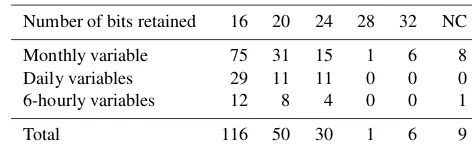
Table 2.The number of variables that used eachfpzipcompression level (in terms of number of bits retained). Note that NC means “not compressed” due to missing values.
Number of bits retained 16 20 24 28 32 NC
Monthly variable 75 31 15 1 6 8 Daily variables 29 11 11 0 0 0 6-hourly variables 12 8 4 0 0 1
Total 116 50 30 1 6 9
that when applying the customized-by-variablefpzip param-eters to a single CESM-LE ensemble member (180 simula-tion years) yielded an average CR of 0.18 (more than a 5 : 1 reduction), which is a 3.5 times reduction over the lossless NetCDF4 library compression. The third row in Table 1, la-beled “truncation”, indicates the compression ratios possi-ble with simple truncation if each variapossi-ble was truncated to the same precision as specified forfpzip. (Table 2 lists how many variables out of the 212 total used each level offpzip compression). Therefore, the differences between the com-pression ratios forfpzipand truncation in Table 1 highlight the added value offpzip’s predictor and encoder in reducing data volumes over simple truncation. Note that Table 2 shows that the majority of the variables were able to use the most aggressive compression,fpzip-16.
4 Ensemble data evaluations
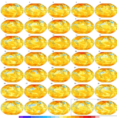
Figure 1.CVDP-generated global maps of historical (1920–2012) annual surface air temperature trends for the 30 original individual CESM-LE ensembles member, the three new members (31–33), and the reconstructed data from new members 31 and 33 (contained in the lower right box).
4.1 CVDP
We first discuss results from the Climate Variability Diag-nostic Package (CVDP) (Phillips et al., 2014), a publicly available analysis tool for examining major modes of cli-mate variability. In particular, the CVDP outputs a vari-ety of key climate metrics, which are immediately viewable via a website of images (means, standard deviations, cou-pled modes of variability, atmospheric modes of variabil-ity, global trend maps, AMOC (Atlantic Meridional Over-turning Circulation), time series data, etc.). The CVDP was used to document the climate simulated by each mem-ber of the CESM-LE, and complete CVDP diagnostic data and images from several time periods are available on the CESM-LE project diagnostics page (http://www.cesm.ucar. edu/experiments/cesm1.1/LE/). Global trend maps are one of the key metrics in the CVDP, and in Fig. 1, we show the CVDP-generated global trend map for annual air
4.2 Climate characteristics
We now describe an analysis aimed at determining whether the effects of the lossy compression could be distinguished from the internal variability inherent in the climate model as illustrated by the CESM-LE project ensemble member spread. The CESM-LE historical simulation (1920–2005) data are examined for ensemble members 2–33 (member 1 is excluded due to a technicality related to its different starting date). Multiple characteristics of interest across the ensemble are examined: surface temperature, top-of-the-atmosphere (TOA) model radiation, surface energy balance, precipitation and evaporation, and differenced temperature fields. The ef-fects of compression are discernable in several characteris-tics.
4.2.1 Surface temperature
First, we plot the global mean annual surface temperature evolution in Fig. 2. Because the three additional members (31–33) are within the range of internal variability, this plot does not indicate which new member(s) has been compressed and reconstructed. Second, we examine the extreme values for surface temperature due to the often cited concern that applying compression to scientific data could dampen the extremes. We calculate the difference between the maxi-mum monthly average and minimaxi-mum monthly average sur-face temperature in 3-year segments. While the temperature difference was the lowest for member 32 (which was not compressed) in the first 6 years, this trend did not continue through the remaining 80 years. In fact, none of the members 31–33 show any detectable surface temperature anomalies as compared to the rest of the ensemble members.
4.2.2 Top-of-the-atmosphere model radiation
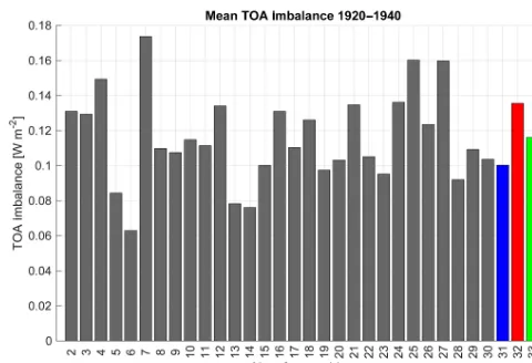
Examining the TOA model radiation balance is of interest as compression could potentially violate conservation of mass, energy or momentum. TOA imbalance is calculated as net shortwave (SW) radiation minus the net longwave (LW) diation. We found no discernable difference in the TOA ra-diation imbalance due to compression (that could be distin-guished from the ensemble variability) when we looked at members 1–33 in the time period 1920–2005 or the shorter period from 1920 to 1940, shown in Fig. 3. Furthermore, the TOA radiation imbalance time series in Fig. 4 also indicates that internal variability is masking any possible effects due to compression. Note that we also examined the top of the model net LW and net SW radiation independently and that data did not indicate any anomalies in the new members ei-ther.
4.2.3 Surface energy balance
Surface energy balance is another popular climate model characteristic that is commonly calculated in climate model
Figure 2.Annual global mean surface temperature evolution for 1920–2005. CESM-LE members 2–30 are indicted in gray and the three new members (31–33) are designated in the legend. Note that members 31 and 33 have been subjected to lossy compression.
Figure 3. Global mean of top-of-model energy imbalance from 1920 to 1940 for CESM-LE members 2–30 and the three new mem-bers (31–33). Note that memmem-bers 31 and 33 have been subjected to lossy compression.
Figure 4. Top-of-model energy imbalance from 1920 to 2005. CESM-LE members 2–30 are indicted in gray and the three new members (31–33) are designated in the legend. Note that mem-bers 31 and 33 have been subjected to lossy compression.
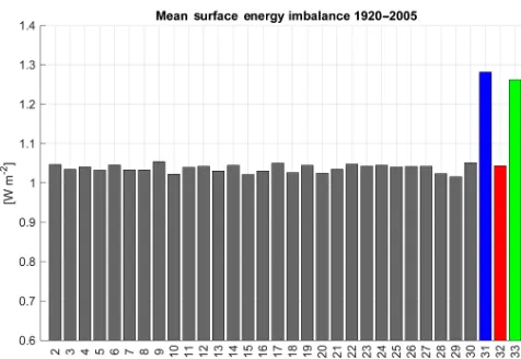
Figure 5.Mean surface energy imbalance from 1920 to 2005 for CESM-LE members 2–30 and new members 31–33. Note that members 31 and 33 have been subjected to lossy compression.
of internal variability. We found that the difference in surface energy balance for 31 and 33 is attributable to lower levels of the LHFLX for the reconstructed members, as seen in Fig. 6. We note that this larger surface energy imbalance persists in the later CESM-LE sets from 2006 to 2080.
We examined the four CESM-LE variables involved in the surface energy balance calculation. We found that LHFLX was compressed more aggressively than the other three vari-ables (fpzip-16 vs.fpzip-24). Therefore, we repeated the sur-face energy balance calculation with LHFLX subjected to fpzip-24 (instead offpzip-16) and found that the surface
en-Figure 6.Mean surface latent heat flux (LHFLX) from 1920 to 2005 for CESM-LE members 2–30 and new members 31–33. Note that members 31 and 33 have been subjected to lossy compression.
Figure 7.Mean surface energy imbalance from 1920 to 2005 for CESM-LE members 2–30 and new members 31–33 with adjusted compression level (fpzip-24) for LHFLX. Note that members 31 and 33 have been subjected to lossy compression.
ergy balance anomalies for members 31 and 33 disappear. Figure 7 shows the new result. Clearly relationships between variables can be important when determining an appropriate amount of compression to apply, especially in the context of derived variables. We further discuss this lesson in Sect. 6. 4.2.4 Precipitation and evaporation
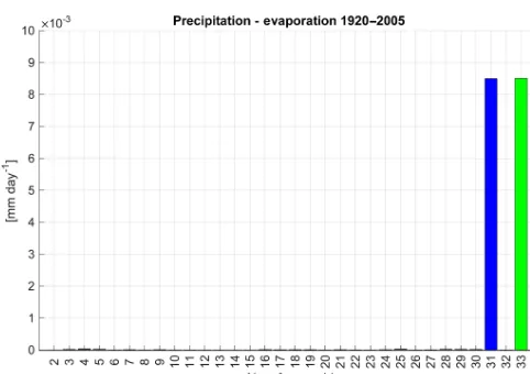
deter-Figure 8. Mean precipitation from 1920 to 2005 for CESM-LE members 2–30 and new members 31–33. Note that members 31 and 33 have been subjected to lossy compression.
Figure 9.The balance between precipitation and evaporation from 1920 to 2005 for CESM-LE members 2–30 and new members 31– 33. Note that the compression level for LHFLX isfpzip-16 (in con-trast to Fig. 10). Also, members 31 and 33 have been subjected to lossy compression.
mined from the first ensemble member (such that precipita-tion and evaporaprecipita-tion were equal). A look at the evaporaprecipita-tion across the ensemble showed lower levels of evaporation cor-responding to members 31 and 33, resulting in the precipita-tion/evaporation imbalance shown in Fig. 9.
Both PRECC and PRECL were compressed with fpzip -24, whereas LHFLX usedfpzip-16. As with the previously discussed surface energy balance calculation, the size of the anomalies in Fig. 9 points to the issue of a derived variable calculated from variables with differing levels of compression-induced error. Therefore, if we redo the pre-cipitation/evaporation imbalance using LHFLX compressed withfpzip-24, the discrepancy between members 31 and 33 and the rest of the ensemble disappears, e.g., Fig. 10.
Figure 10.The balance between precipitation and evaporation from 1920 to 2005 for CESM-LE members 2–30 and new members 31– 33 with adjusted compression level for LHFLX (fpzip-24). Note the difference in scale between this plot and that in Fig. 9. Also, mem-bers 31 and 33 have been subjected to lossy compression.
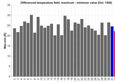
4.2.5 Differenced temperature field
would be problematic. We calculated the difference between the minimum and maximum values in the differenced tem-perature field for each ensemble member for every month from 1920 to 2005. This calculation characterizes the largest temperature gradients that occur for each month. We show the October 1920 results in Fig. 11, which indicate that noth-ing is amiss with members 31 and 33 (which was also the case for all of the other months from 1920 to 2005).
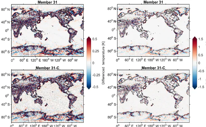
In general, though, determining whether compression caused an overall smoothing effect on the data is perhaps bet-ter viewed by examining spatial contrast plots showing the north–south and east–west differences for the near-surface air temperature for the ensemble members. For ensemble member 31, Fig. 12 shows both the original (labeled “mem-ber 31”) and reconstructed (labeled “mem“mem-ber 31-C”) data from October of 1920. Note that the scale of the color bar would need to be greater than±10◦to represent all gradients, but at that scale differentiating the smaller gradients is diffi-cult and no compression effects can be detected. Therefore, the rightmost plots in Fig. 12 have a color bar scale tightly re-stricted to±0.5◦. At this restricted scale, one can notice the effects of lossy compression largely over the ocean in areas where the original gradient was quite small already. How-ever, when the color scale is slightly expanded to±1.5◦(in the leftmost plots), it is difficult to discern any differences be-tween 31 and 31-C, and the larger gradients over land coast-lines and ridges dominate, as expected.
4.3 Ensemble variability patterns
The idea behind the following analysis was to deter-mine whether lossy compression would introduce detectable small-scale variability patterns into the climate data. To this end, we reconstructed each large ensemble member (1–33) from a basis set derived from the variability from each other member of the large ensemble, with the idea that the complete basis set derived from the compressed members would be able to explain less variance in the other simula-tions (because some of the higher modes would not be well-represented).
In particular, we followed the following procedure. For each ensemble member (1–33), we did a singular value de-composition (SVD) analysis to determine the EOFs (empir-ical orthogonal functions) in the spatial dimension on the monthly temperature field for 900 months. Note that we ex-amined a subset of the grid cells to reduce computational costs. We then projected each of the remaining 32 ensem-ble members onto the resulting EOF basis and calculated the unexplained variance. Figure 13 provides the sum of the un-explained variance (mean squared error) in temperature for each ensemble member (note that the expectation value has been subtracted for clarity). Figure 13 indicates that mem-bers 31 and 33 are outliers, meaning that their set of EOFs is less appropriate as a basis set to describe the variability in the other ensemble members; this is due to loss of precision
Figure 11.Difference between maximum and minimum values oc-curring in the neighbor-differences surface temperature field (TRE-FHT) for each ensemble member for October 1920. Note that mem-bers 31 and 33 have been subjected to lossy compression.
induced by lossy compression (which primarily affects the high-frequency modes).
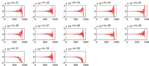
Figure 14 shows the same result in an alternative way. Each subplot uses a set of EOFs (900 total) derived from a member of the large ensemble (subplots are only shown for members 21–33, as 1–20 share similar characteristics to the other members not subject to compression). The remain-ing 32 members are projected onto the EOF basis set, and we calculate the variance of the principal components in the rest of the ensemble (900×32 samples). The anomaly of this curve relative to the ensemble mean case is plotted in the sub-plots in Fig. 14. The subplotxaxes represent the 900 EOFs, and the y axes indicates the magnitude of the temperature variance. The subplots for ensemble members 31 and 33 in-dicate that when the rest of the ensemble members projected onto their EOFs, those modes of rank 500 or greater exhibit lower than expected variance. Again, the reconstructed mem-bers do not contain the high-frequency information present in the rest of the ensemble. Of note is that when we alterna-tively first derived EOFs in members 1–30 and then projected members 31 and 33 onto that basis set, no differences were detected as expected. Given that the differences are only no-ticeable in the higher EOFs (which are not typically exam-ined), it appears that the compressed members are not (no-ticeably) under-representing any of the true modes of vari-ability.
Figure 12. A comparison of the difference maps (i.e., gradients) for the surface temperature field (TREFHT) for ensemble members 31 (original) and 31-C (reconstructed) for October 1920. Note that the color scale for the left maps has a smaller range than for the right maps.
Figure 13.The sum of the mean squared error in temperature field when the other ensemble members’ variance is projected onto a sin-gle member’s EOF basis. Note that members 31 and 33 have been subjected to lossy compression.
extreme temperatures or precipitation. We partially address this issue in Sect. 5.1 by investigating the extremes. However, in future work we will further explore whether compression-induced damping of high-frequency elements (spatially or temporally) has relevant effects that exceed the noise stem-ming from the model’s floating-point calculations.
4.4 Coherent structures
4.4.1 Overview of proper orthogonal decomposition Proper orthogonal decomposition (POD) is used for the ex-traction of coherent structures, or the study of recurring pat-terns in spatiotemporal fields. The POD technique was first introduced in the context of fluid turbulence by Lumley (1967) in order to analyze the velocity field of fluid flows. POD has since been adapted for use within a number of different disciplines, such as oceanography, chemistry, and model-order reduction (Carbone et al., 2011). The aim of POD is to provide an optimal basis set to represent the dy-namics of a spatiotemporal field, which allows for the iden-tification of theessential informationcontained in the signal by means of relatively few basis elements (modes).
In particular, given a spatiotemporal field I (x, t ), POD calculates a set of modes8in a certain Hilbert space adapted to the fieldI (x, t )such that
I (x, t )= ∞ X
i=1
ai(t )φi(x), (2)
whereai(t )is a time-varying coefficient. From a mathemati-cal point of view, POD permits the maximization of the pro-jection of the fieldI (x, t )on8:
Maxφih(I (x, t ), φi(x))i
(φi(x), φi(x))
. (3)
This defines a constrained Euler–Lagrange maximization problem, the solution of which is a Fredholm integral equa-tion of the first kind:
Z
Figure 14.The subplotxaxes represent the 900 EOFs. Theyaxes indicate the magnitude of the temperature variance. The ensemble member number is indicated in each subplot title, and members 31 and 33 have been subjected to lossy compression.
where(a, b)is the inner product, angle brackets indicate the time average,is the spatial domain,φi(x)is an eigenfunc-tion, andλi is a real positive eigenvalue. If the spatial domain
is bound, this decomposition provides a countable, infinite, set of sorted eigenvaluesλi (withλ1≥λ2≥λ3≥...). Then the field “energy”, by the analogy with the fluid turbulence application, can be written as
hI (x, t )i = ∞ X
n=1
λi, (5)
whereλi represents the average energy of the system pro-jected onto the axisφi(x)in the eigenfunction space. In gen-eral, the eigenfunction φi(x)does not depend on the func-tions of the linearized problem, but emerges directly from the observations of the fieldI (x, t ). When the sum in Eq. (2) is truncated toN terms, it contains the largest possible energy with respect to any other linear decomposition belonging to the family of EOFs (i.e., PCA, SVD) of the same truncation order (Lumley, 1967).
4.4.2 Application to ensemble data
For this study, we utilize POD to investigate whether lossy compression introduced any detectable artifacts that could indicate which ensemble member(s) of the new set 31–33 had been compressed and to determine whether any such ar-tifacts were acceptable or not (i.e., in terms of impact on the physics of the problem). We examined the monthly averaged output of four variables:Z3 (geopotential height above sea level), CCN3 (cloud condensation nuclei concentration), U
(zonal wind), and FSDSC (clear-sky downwelling solar flux at surface). For each variable and for each ensemble member (1–33), POD was applied to a period of 25 years (300 time slices beginning with January 2006) to obtain the modes and the energy associated with each mode. This methodology en-ables the identification of any perturbations introduced by the compression method into the dynamics of the field. In addi-tion, we can characterize the impact of the compression, if
any, with respect to the inherent variability within the en-semble.
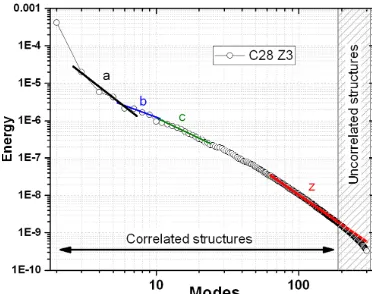
To illustrate this process, the “energy” fractionλas a func-tion of the mode numberN is reported in Fig. 15 for variable
Z3 from ensemble member 28. Note that the distribution ofλ
is composed of different branches (groups of modes) charac-terized by a power-law behavior. The first branches (a, b, and c) represent the dominant scales (structures) in the field and contain the greater part of the energy of the original field. These structures can be considered mother structures, and, analogously to the fluid turbulence case, they represent the “energy injection” point for the smaller structures. In other words, the large-scale structures transfer energy to smaller-and-smaller-scale structures. When a break is found in the distribution, the energy transfer is stopped, and a new cas-cade begins that is unrelated to the previous one. For the highest modes (∼scale of the resolution) the energy is quite low, and the modes have a minimal impact on the “physics”. Beyond this point the modes can be considered uncorrelated noise, which is generally associated with the thermal noise of the floating-point calculations, rather than anything phys-ically meaningful. Therefore, by comparing the energy dis-tribution of the decomposition modes of the new ensemble members 31–33 with their inherent variability, it should be possible to both identify the presence of any perturbations due to the compression algorithm as well as the scale at which the perturbations are significant.
Figure 15.Energy distribution of the modes of the POD for variable Z3 for ensemble member 28. Superimposed power laws indicate the “energy cascades” in correlated modes, and three principal scales are present: a, b, and c. The limit of the cascade is labeled z, and the shaded area indicates modes associated with noise.
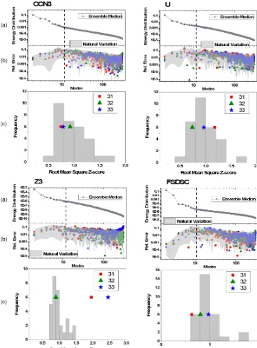
for the original ensemble members together with the RMSZ of the energy distribution of members 31–33. The plot cor-responding to variableZ3 in Fig. 16 clearly shows that the RMSZ values for members 31 and 33 are outliers in Fig. 16c, suggesting that there are some artifacts in the distribution en-ergy of the modes of their relative PODs, potentially caused by lossy compression. However, when comparing these er-rors with the natural variability observed within the original ensemble, it appears clear that such anomalies are mainly visible in the lowest energy modes (>150). Since the low-est energy modes are generally attributed to thermal noise in floating-point calculations, if these artifacts are due to lossy compression, they do not affect any coherent structures at-tributable to the physics of the problem (i.e., the climate). Note that ensemble members 31 and 33 for variablesUand FSDSC exhibit errors in the energy distribution that in a few instances exceed the natural variability within the ensemble as shown in Fig. 16b, but the exceedance is not great enough to clearly indicate them as outliers in Fig. 16c. (Recall that ensemble member 32 was not compressed.) Finally, the er-rors in the energy distribution of the modes of the decompo-sition for ensemble members 31–33 for variable CCN3 are well within the variation explained by the natural variability of the original ensemble members, and therefore no outliers were observed.
This analysis performed on a limited number of variables shows that the compression of the ensemble members has either no effect if compared with the natural variability ob-served within the ensemble, or (forZ3) affects only the low-est energy modes. We note that the outcome of this analy-sis could potentially be different if applied to higher tempo-ral resolution output data as lossy compression could impact finer scale patterns differently.
5 The original and reconstructed data
In this section, we describe analyses performed on the CESM-LE data that were conducted with the knowledge that members 31 and 33 had been compressed and reconstructed. In addition, we provided both the original and reconstructed versions of 31 and 33 for these experiments.
5.1 Climate extremes
5.1.1 Overview of extreme value theory
Extreme value theory, as the name implies, focuses on ex-tremes, more precisely on the upper tail distributional fea-tures. For extremes, the Gaussian paradigm is not applicable. To see this, suppose that we are interested in annual max-ima of daily precipitation. In this case, the probability density function (pdf) is skewed, bound by zero on the left side, and very large values (greater than two standard deviations) can be frequently observed. These three features cannot be cap-tured by a normal distribution and other statistical modeling tools are needed.
One classical approach is to study block maxima, e.g., the largest annual value of daily temperatures. In this example, the block size is 365 days. The statistical analysis of block maxima is based on the well-developed extreme value theory (EVT), originating from the pioneering work of Fisher and Tippett (1928) and regularly improved upon during the last decades (e.g., De Haan and Ferreira, 2005). This theory indi-cates that the generalized extreme value (GEV) distribution represents the ideal candidate for modeling the marginal dis-tribution of block maxima. This probabilistic framework is frequently applied in climate and hydrological studies deal-ing with extremes (e.g., Zwiers et al., 2013; Katz et al., 2002). Presently, more complex statistical models, such as the mul-tivariate EVT (e.g., De Haan and Ferreira, 2005; Beirlant et al., 2004; Embrechts et al., 1997), also provide a theo-retical blueprint to represent dependencies among maxima recorded at different locations. For this work, however, we will not address the question of spatial dependencies for ex-tremes. We assume that every grid point can be treated inde-pendently and a GEV can be fitted at each location.
Mathematically, the GEV is defined by its three-parameter cumulative distribution function (cdf):
G(y)=exp −
1+ξy−µ σ
−1/ξ
+ !
, (6)
whereµ,σ >0 andξare called the location, scale and shape parameter with the constraint that 1+ξy−µσ >0. Theξ pa-rameter defines the tail behavior with three possible types:
ξ=0 (Gumbel),ξ >0 (Fréchet) andξ <0 (Weibull). Tem-perature extremes often follow a Weibull distribution (e.g., Zwiers et al., 2013). In particular, a negative shape param-eter implies a finite upper bound given byµ−σ
Figure 16.For each of the four variables studied, we show the following:(a)energy distribution of the modes of the POD for ensemble members 31–33, superimposed on the median of the original ensemble members (1–30);(b)relative errors of the energy distributions of the modes of the POD for new ensemble members 31–33 and the median of the original ensemble together with the natural variability observed within the uncompressed ensemble;(c)RMSZ distribution of the energy distribution for the 30 members of the original ensemble together with the RMSZ score of the energy distribution of new members 31–33. Note that members 31 and 33 have been subjected to lossy compression.
to model daily maxima of methane (Toulemonde et al., 2013) and precipitation maxima are often described by a Fréchet distribution (see, e.g., Cooley et al., 2007). In terms of risk analysis, the scalarξ is the most important parameter of the
Figure 17.GEV shape parameterξvariability; see Eq. (6). The left, middle, and right panels correspond to the pdf ofξ, its range among compressed runs, and its difference between a compressed and uncompressed run, respectively. The four variables shown are TSMN (min-imum surface temperature), TSMX (max(min-imum surface temperature), PRECT (average convective and large-scale precipitation rate), and PRECTMX (maximum convective and large-scale precipitation rate).
5.1.2 Application to ensemble data
We focus our analysis on four variables from the ensemble data: average convective and large-scale precipitation rate (PRECT) over the output period, maximum convective and large-scale precipitation rate (PRECTMX), minimum
including MLE (maximum likelihood estimation), MOM (method of moments), and Bayesian methods, can be used. As the shape parameter for precipitation and temperatures extremes is classically between −0.5 and 0.5, we opt for the probability-weighted moments (PWMs) (e.g., Ana and de Haan, 2015), which has a long tradition in statistical hy-drology (e.g., Landwehr et al., 1979; Hosking and Wallis, 1987) and has been applied in various settings (e.g., Toreti et al., 2014). Besides its simplicity, the PWMs approach usu-ally performs reasonably well compared to other estimation procedures (e.g., Caeiro and Gomes, 2011). Additional argu-ments in favor of PWMs are that they are typically quickly computed, an important feature in our setup, and do not pro-vide aberrant values for negative ξ like the MLE. To apply this estimation technique to temperature min and max, global warming trends have to be removed. This was done by re-moving the trend with a local non-parametric regression (us-ing theloessfunction inR).
Figure 17 summarizes our findings concerning the shape parameterξ. Each row represents a variable of interest. We only show results for one of the two compressed ensem-ble members as the results are practically identical. The his-tograms correspond to the empirical pdf obtained from all uncompressed runs. This can be compared to the blue pdf of the compressed run. For our four atmospheric variables, one cannot make the distinction between the compressed and un-compressed runs, which indicates that compression did not systematically change the distribution of the shape parame-ters. The middle panels display the range of the estimatedξat each grid point from the ensemble of 31 uncompressed runs. This gives us information on the variability among the 31 un-compressed runs, which can be compared to the difference between a compressed run and its uncompressed counterpart (the right panels). As indicated by the dark blue color (mean-ing low values), the ensemble variability is much higher than the variability due to compression. In summary, this analy-sis indicates that compression does not cause any systematic change in the distribution of the estimated shape parame-ters and that the changes introduced by compression fall well within the variability of the ensemble.
5.2 Causal signatures
The goal of causal discovery in this context is to identify potential cause–effect relationships from a dataset to better understand or discover the dynamic processes at work in a system. Causal discovery tools have been developed from probabilistic graphical models (e.g., detailed in Pearl, 1988 and Spirtes et al., 2000), which are a graphical represen-tation of probable dependencies between variables in high-dimensional space. In particular, causal discovery methods reveal more than simply correlation, but rather the patterns of information flow and interactions. To determine the flow of information, the initial assumption is made that every able (graph node) is causally connected to every other
vari-able. Then conditional independence tests (e.g., testing for vanishing partial correlations) are used to disprove causal connections, resulting in a remaining “interaction map” of causal connections (that may or may not be given direction through additional techniques). Such tools were initially ap-plied in the fields of social sciences and economics, but have more recently been applied successfully to climate science data (e.g., Chu et al., 2005; Ebert-Uphoff and Deng, 2012a, b; Zerenner et al., 2014). For example, for atmospheric data, one could imagine using causal discovery methods to under-stand large-scale atmospheric processes in terms of informa-tion flow around the earth.
Of interest here is determining whether compressing the climate data in the CESM-LE dataset affected the flow of information. Using causal discovery for this purpose is pro-posed in Hammerling et al. (2015), where interaction maps were generated for both the original and reconstructed data. We call these interaction maps causal signatures. This type of analysis is unique to this compression study as it is aimed at inter-variable relationships. Recall that the number of daily variables contained in the CESM-LE datasets is 51. To sim-plify the analysis, we created a subset of 15 daily variables. The subset was chosen such that only one variable was kept from each like-variable group. For example, eight of the 51 total daily variables report temperature in some form: at several defined pressure surfaces, at the surface, and at a near-surface reference height (TREFHT); therefore, we only include the temperature variable TREFHT in the subset. We then developed temporal interaction maps for the 15 daily variables that show interactions across different lag times be-tween variables. We performed this analysis for several dif-ferent temporal scales, i.e., we identified separate signatures considering lag times between variables that are multiples of 1, 5, 10, 20, 30, or 60 days, in order to capture interac-tions for example on a daily (1 day) or monthly (30 days) scale. Recall that these interaction maps are highlighting po-tential cause–effect relationships. Figure 18 contains the in-teraction map for the daily timescale (lag times are multiples of 1 day) for the original data for CESM-LE member 31, and the 15 variables are indicated in the ovals. Note that only the weak connection between SHFLX (surface sensible heat flux) and FSNTOA (net solar flux at top of atmosphere), which is indicated by a dotted line, is missing in the map corresponding to the reconstructed data. In general, the maps for all of the lagged times only indicatedtinydifferences be-tween the initial and reconstructed datasets. This result in-dicates that compressing and reconstructing the climate data has not negatively impacted the flow of information in terms of detectable cause–effect relationships in the data.
5.3 AMWG diagnostics package
Figure 18.Causal signature interaction map for CESM-LE member 31. Blue lines delineate instantaneous connections and red lines indicate connections with a time lag. The number(s) next to each line give the number of days from potential cause to potential effect. The single dotted line between SHFLX and FSNTOA indicates a very weak instantaneous connection. Note that the causal signature for reconstructed CESM-LE member 31C is identical to this figure, except that the weak connection between SHFLX and FSNTOA is no longer present.
CAM and produces plots and tables of the mean climate in a variety of formats. The AMWG-DP uses monthly output to evaluate climate characteristics such as seasonal cycles, intraseasonal variability, Madden–Julian Oscillation (MJO), El Niño–Southern Oscillation (ENSO), and the diurnal cy-cle. The AMWG-DP can be used to compare model simula-tion output of observasimula-tional and reanalysis data or to compare output from two simulations. Therefore, comparing the com-pressed and reconstructed CESM-LE ensemble members via the AMWG-DP is a natural choice. Note that the AMWG-DP is available at https://www2.cesm.ucar.edu/working-groups/ amwg/amwg-diagnostics-package.
Because the AMWG-DP produces over 600 tables and plots, we just highlight a couple of results here. First we show vertical contour plots produced by the AMWG-DP (from diagnostics set 4) comparing the original and reconstructed variants of ensemble member 31 for relative humidity (REL-HUM) in Fig. 19. We chose to look at RELHUM because it was compressed aggressively withfpzip-16, yielding a CR of 0.09. While the max values are not identical (101.66 vs. 101.86), the contour plots certainly appear very similar at this scale.
Now we show surface pressure (PS), as it is a “popu-lar” variable to view with the AMWG-DP. Variable PS was compressed withfpzip-20, yielding a CR of 0.13. Figure 20 compares the original and reconstructed variants of ensem-ble member 31 via horizontal contour plots (from diagnos-tics set 5). Note that while the mean, max, and min values differ slightly, the plots themselves are indistinguishable and similar conclusions could be drawn.
Finally, we look at a portion of one of the AMWG-DP tables for global annual means for the 2006–2099 data
Figure 19. Vertical contour plot of DJF (December–January– February) zonal means for relative humidity (RELHUM) from 2006 to 2099 for ensemble member 31. The data in the left subplot have undergone lossy compression (i.e., 31-C) and the right subplot con-tains the original data.
How-Figure 20. Horizontal contour plot of DJF (December–January– February) means for surface pressure (PS) from 2006 to 2099 for ensemble member 31. The data in the top subplot have undergone lossy compression (i.e., 31-C) and the bottom subplot contains the original data.
Table 3.Subset of AMWG diagnostics set 1: annual means global. RESTOM and RESSURF are AMWG-DP-derived variables for the top-of-model residual energy balance and the surface residual en-ergy balance, respectively. RMSE indicates the root mean squared error. Units are W m−2.
Variable Compressed Original Difference RMSE case case
RESTOM 2.016 2.016 0.000 0.001 RESSURF 1.984 1.984 0.000 0.000
ever, this simple diagnostic calculation warrants further dis-cussion. We note that compressing FSNT withfpzip-16 and FLNT withfpzip-20 was acceptable in terms of passing the four quality metrics used to determine compression levels (see discussion in Sect. 3). However, because we knew in ad-vance of applying compression that calculating the top of the model balance (FSNT−FSLT) is a key diagnostic check for climate scientists, we preemptively used less aggressive com-pression for both variables (as subtracting like-sized quanti-ties would magnify the error due to compression). For exam-ple, had we instead used FSNT withfpzip-16 and FLNT with fpzip-20, this would have resulted in relative errors of 0.3 and 0.02 % for FSNT and FLNT, respectively, but in a relative er-ror for the derived quantity RESTOM of 8.0 %, which is no-ticeably larger (corresponding to RESTOM values of 7.553 and 8.211 W m−2).
The AMWG-DP-derived quantity RESSURF for surface residual energy balance in Table 3 is notably on target in the
compressed data. In contrast, when the surface energy bal-ance was investigated in Sect. 4.2.3, Fig. 5 indicated that the effects of compression were noticeable in the surface energy calculation (due to aggressive compression of the surface latent heat flux, LHFLX). In both Sect. 4.2.3 and AMWG-DP, the surface energy balance was calculated as (FSNS−FLNS−SHFLX−LHFLX). However, the differ-ence is that the AMWG-DP does not use the LHFLX vari-able from the output data, but instead calculates surface latent heat flux via surface water flux (QFLX) and four precipita-tion variables (PRECC, PRECL, PRECSC, and PRECSL). As a result, compression of variable LHFLX did not affect the AMWG-DP’s calculation of surface energy balance.
6 Lessons learned
By providing climate scientists with access to data that had undergone lossy compression, we received valuable feed-back and insights into the practicalities of applying data com-pression to a large climate dataset. Here we summarize the underlying themes or lessons that we learned from this lossy compression evaluation activity.
6.1 Relationships between variables
When determining appropriate levels of compression, rela-tionships between variables can be an important considera-tion, particularly in the context of derived variables. As an example, we refer to the surface energy balance anomaly de-tected and discussed in Sect. 4.2.3. Had all four variables been compressed to the same precision, the surface energy balance in the reconstructed members would not have stood out (i.e., Fig. 5 vs. Fig. 7). Derived variables are quite popu-lar in post-processing analysis, and it is unrealistic to expect to know how the output data will be used at the time it is generated (and compressed). However, many derived vari-able calculations are quite standard (surface energy balance, TOA energy balance, etc.), and these often-computed derived variables should be considered when determining appropri-ate levels of compression for variables used in their calcula-tions.
6.2 Detectable vs. consequential
and detect a warming trend. On the other hand, one may not want to study high-frequency scale events such as precipita-tion with data that have undergone aggressive compression. In general, understanding the precision and limitations of the data being used is critical to any post-processing analysis. 6.3 Individual treatment of variables
We confirmed the assertion in Baker et al. (2014) that de-termining the appropriate amount of compression must be done on a variable-by-variable basis. In particular, there is not a “one-size-fits-all” approach to compressing climate simulation variables, and it does not make sense to assume that 32 bits is the right precision for every variable. Fur-ther, customizing compression per variable could also in-clude applying other types of compression algorithms to dif-ferent variables as well (e.g., transform-based methods such as wavelets), which is a topic of future study. Knowing what precision is needed for each variable for CESM, or even more generally for CMIP (discussed in Sect. 1), would clearly fa-cilitate applying lossy compression. We note that defining such a standard is non-trivial and would need to be fluid enough to accommodate new variables and time/space res-olutions.
6.4 Implications for compression algorithms
Achieving the best compression ratio without negatively im-pacting the climate simulation data benefits from a thorough understanding how a particular algorithm achieves compres-sion. For example, we are aware that the type of loss in-troduced by fpzipis of the exact same kind that is already applied to the original double-precision (64 bit) data when truncating (or, more commonly, rounding) to single precision (32 bit) for the CESM history file. Because of its truncation approach,fpzipis much less likely to affect extreme values or have a smoothing effect on the data, as opposed to, for example, a transform-based approach.
Further, Fig. 6 illustrates that naive truncation is not ideal. An improvement would be to inject random bits or at least round rather than truncate the values (i.e., append bits 100. . .0 instead of bits 000. . .0 to the truncated floats). Both of these modifications could be done as a post-processing step after the data have been reconstructed. Although the temperature gradients (as shown in Fig. 11) are not problem-atic in this study, injecting random bits would also reduce the number of zero gradients. On a related note, a compression algorithm that provides information about the compression error at each grid point could potentially be very useful in terms of customizing how aggressively to compress particu-lar climate simulation variables.
Finally, an important issue for climate data is the need for compression algorithms to seamlessly handle both miss-ing values and fill values. As mentioned previously, vari-ables that occasionally have no value at all (i.e., missing)
at seemingly random grid points require special handling by the compression algorithm itself or in a pre- and/or post-processing step. Similarly, the non-regular presence of large-magnitude fill values (typicallyO(1035)in CESM) can be problematic as well.
7 Concluding remarks
In general, lossy data compression can effectively reduce climate simulation data volumes without negatively impact-ing scientific conclusions. However, by providimpact-ing climate re-searchers with access to a large dataset that had undergone compression (and soliciting feedback), we now better appre-ciate the complexity of this task. All of the lessons detailed in the previous section highlight the importance of being data and science aware when applying data compression and per-forming data analysis. To reap the most benefit in terms of achieving low compression ratios without introducing sta-tistically significant data effects requires an understanding of the characteristics of the data, their science use, and the properties (i.e., strengths and weaknesses) of the compres-sion algorithm. In fact, many considerations for applying lossy compression to climate simulation data align with those needed to carefully choose grid resolution, data output fre-quency, and computation precision, all of which effect the validity of the resulting simulation data. Further, our com-pression research thus far has focused on evaluating individ-ual variables, and this study highlights that issues can arise when compressing multiple variables or using derived vari-ables. Our ongoing research on compression methods will focus on incorporating the multivariate aspects of compres-sion and ultimately developing a tool to auto-determine ap-propriate compression (and therefore acceptable precision) for a given variable.
8 Code and data availability
Appendix A: Lossy compression evaluations
Table A1 lists which co-authors conducted the ensemble data evaluations described in Sects. 4 and 5.
Table A1.A list of co-authors and their corresponding evaluations.
Section Type of evaluation Author(s)
4.1 CVDP Sheri A. Mickelson, Jennifer E. Kay 4.2 Climate characteristics Martin B. Stolpe
4.3 Ensemble variability patterns Ben Sanderson
4.4 Coherent structures Francesco De Simone, Francesco Carbone, Christian N. Gencarelli 5.1 Climate extremes Phillipe Naveau
Acknowledgements. We thank Adam Phillips (NCAR) for his input on CVDP. We thank Reto Knutti (ETH Zurich) for his suggestions and ideas. We also thank William Kaufman (Fairview HS) for his work on Fig. 17. This research used computing resources provided by the Climate Simulation Laboratory at NCAR’s Computational and Information Systems Laboratory (CISL), sponsored by the National Science Foundation and other agencies. Part of this work has been supported by the ANR-DADA, LEFE-INSU-Multirisk, AMERISKA, A2C2, and Extremoscope projects. Part of the work was done during P. Naveau’s visit to IMAGe-NCAR in Boulder, CO, USA. Part of this work was performed under the auspices of the U.S. Department of Energy by Lawrence Livermore National Lab-oratory under contract DE-AC52-07NA27344, and this material is based upon work supported by the U.S. Department of Energy, Of-fice of Science, OfOf-fice of Advanced Scientific Computing Research.
Edited by: J. Annan
Reviewed by: two anonymous referees
References
Ana, F. and de Haan, L.: On the block maxima method in extreme value theory, Ann. Stat., 43, 276–298, 2015.
Baker, A., Xu, H., Dennis, J., Levy, M., Nychka, D., Mickelson, S., Edwards, J., Vertenstein, M., and Wegener, A.: A Methodol-ogy for Evaluating the Impact of Data Compression on Climate Simulation Data, in: Proceedings of the 23rd International Sym-posium on High-performance Parallel and Distributed Comput-ing, HPDC ’14, 23–27 June 2014, Vancouver, Canada, 203–214, 2014.
Baker, A. H., Hammerling, D. M., Levy, M. N., Xu, H., Dennis, J. M., Eaton, B. E., Edwards, J., Hannay, C., Mickelson, S. A., Neale, R. B., Nychka, D., Shollenberger, J., Tribbia, J., Verten-stein, M., and Williamson, D.: A new ensemble-based consis-tency test for the Community Earth System Model (pyCECT v1.0), Geosci. Model Dev., 8, 2829–2840, doi:10.5194/gmd-8-2829-2015, 2015.
Beirlant, J., Goegebeur, Y., Segers, J., and Teugels, J.: Statistics of Extremes: Theory and Applications, Wiley Series in Probability and Statistics, Hoboken, USA, 2004.
Bicer, T., Yin, J., Chiu, D., Agrawal, G., and Schuchardt, K.: In-tegrating online compression to accelerate large-scale data an-alytics applications. IEEE International Symposium on Parallel and Distributed Processing (IPDPS), 20–24 May 2013, Boston, Massachusetts, USA, 1205–1216, doi:10.1109/IPDPS.2013.81, 2013.
Caeiro, F. and Gomes, M. I.: Semi-parametric tail inference through probability-weighted moments, J. Stat. Plan. Infer., 16, 937–950, 2011.
Carbone, F., Vecchio, A., and Sorriso-Valvo, L.: Spatio-temporal dynamics, patterns formation and turbulence in complex fluids due to electrohydrodynamics instabilities, Eur. Phys. J. E, 34, 1– 6, 2011.
CESM: CESM Models and Supported Releases, available at: http:// www.cesm.ucar.edu/models/current.html, last access: 1 Decem-ber 2016.
Chu, T., Danks, D., and Glymour, C.: Data Driven Methods for Nonlinear Granger Causality: Climate Teleconnection
Mecha-nisms, Tech. Rep. CMU-PHIL-171, Carnegie Mellon University, Pittsburg, PA, USA, 2005.
CMIP5: Coupled Model Comparison Project Phase 5, available at: http://cmip-pcmdi.llnl.gov/cmip5/ (last access: 1 June 2016), 2013.
Cooley, D., Nychka, D., and Naveau, P.: Bayesian Spatial Modeling of Extreme Precipitation Return Levels, J. Am. Stat. Assoc., 102, 824–840, 2007.
Day, C. F., Sanders, C., Clochard, J., Hennessy, J., and Elliott, S.: Guide to the WMO Table Driven Code Form Used for the Representation and Exchange of Regularly Spaced Data In Binary Form, available at: http://www.wmo.int/pages/prog/ www/WMOCodes/Guides/GRIB/GRIB2_062006.pdf (last ac-cess: 2 December 2016), 2007.
De Haan, L. and Ferreira, A.: Extreme Value Theory: An Introduc-tion, Springer Series in Operations Research and Financial Engi-neering, New York, USA, 2005.
Earth System Grid: Climate Data at the National Center for Atmo-spheric Research, available at: https://www.earthsystemgrid.org, last access: 1 December 2016.
Ebert-Uphoff, I. and Deng, Y.: A New Type of Climate Net-work based on Probabilistic Graphical Models: Results of Bo-real Winter vs. Summer, Geophys. Res. Lett., 39, L19701, doi:10.1029/2012GL053269, 2012a.
Ebert-Uphoff, I. and Deng, Y.: Causal Discovery for Climate Re-search Using Graphical Models, J. Climate, 25, 5648–5665, 2012b.
Embrechts, P., Klüppelberg, C., and Mikosch, T.: Modelling Ex-tremal Events for Insurance and Finance, Applications of Math-ematics, vol. 33, Springer-Verlag, Berlin, Germany, 1997. Fisher, R. and Tippett, L.: Limiting forms of the frequency
distri-bution of the largest or smallest member of a sample, P. Camb. Philos. Soc., 24, 180–190, 1928.
GFAS: Global Fire Assimilation System v1.2 documentation, available at: http://www.gmes-atmosphere.eu/about/project_ structure/input_data/d_fire/gfas_versions (last access: 1 June 2016), 2015.
Gomez, L. A. B. and Cappello, F.: Improving Floating Point Com-pression through Binary Masks, in: IEEE BigData, Santa Bar-bara, CA, USA, 2013.
Hammerling, D., Baker, A. H., and Ebert-Uphoff, I.: What can we learn about climate model runs from their causal signatures?, in: Proceedings of the Fifth International Workshop on Climate In-formatics: CI 2015, 22–23 September 2015, Boulder, CO., USA, edited by: Dy, J. G., Emile-Geay, J., Lakshmanan, V., and Liu, Y., 2015.
Hosking, J. R. M. and Wallis, J. R.: Parameter and quantile estima-tion for the generalized Pareto distribuestima-tion, Technometrics, 29, 339–349, 1987.
Huang, X., Ni, Y., Chen, D., Liu, S., Fu, H., and Yang, G.: Czip: A Fast Lossless Compression Algorithm for Climate Data, Int. J. Parallel Prog., 44, 1–20, 2016.
Hübbe, N., Wegener, A., Kunkel, J. M., Ling, Y., and Ludwig, T.: Evaluating Lossy Compression on Climate Data, in: Proceedings of the International Supercomputing Conference (ISC ’13), 16– 20 June 2013, Leipzig, Germany, 343–356, 2013.