Stochastic Complexity and Generalization Error of a Restricted Boltzmann Machine in Bayesian Estimation

Stochastic Complexity and Generalization Error of a Restricted

Boltzmann Machine in Bayesian Estimation

Miki Aoyagi [email protected]

Department of Mathematics, College of Science & Technology Nihon University

1-8-14, Surugadai, Kanda, Chiyoda-ku Tokyo 101-8308, Japan

Editor: Tommi Jaakola

Abstract

In this paper, we consider the asymptotic form of the generalization error for the restricted Boltz-mann machine in Bayesian estimation. It has been shown that obtaining the maximum pole of zeta functions is related to the asymptotic form of the generalization error for hierarchical learning models (Watanabe, 2001a,b). The zeta function is defined by using a Kullback function. We use two methods to obtain the maximum pole: a new eigenvalue analysis method and a recursive blow-ing up process. We show that these methods are effective for obtainblow-ing the asymptotic form of the generalization error of hierarchical learning models.

Keywords: Boltzmann machine, non-regular learning machine, resolution of singularities, zeta function

1. Introduction

A learning system consists of data, a learning model and a learning algorithm. The purpose of such a system is to estimate an unknown true density function from data distributed by the true density function. The data associated with image or speech recognition, artificial intelligence, the control of a robot, genetic analysis, data mining, time series prediction, and so on, are very complicated and usually not generated by a simple normal distribution, as they are influenced by many factors. Learning models for analyzing such data should likewise have complicated structures. Hierarchical learning models such as the Boltzmann machine, layered neural network, reduced rank regression and the normal mixture model are known to be effective learning models. They are, however, non-regular statistical models, which cannot be analyzed using the classic theories of non-regular statistical models (Hartigan, 1985; Sussmann, 1992; Hagiwara, Toda, and Usui, 1993; Fukumizu, 1996).

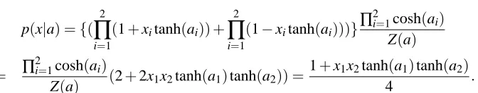
For example, consider a simple restricted Boltzmann machine that has two observable units and one hidden unit with binary variables (Fig. 1). The model is expressed by the probability form of two observable units x= (x1,x2)∈ {1,−1}2_{with a parameter a= (a1,a2)∈R}2_:

p(x|a) =

∑

y=±1

p(x,y|a) =exp(a1x1+a2x2) +exp(−a1x1−a2x2)

Z(a) ,

where y∈ {1,−1}is the hidden variable,

p(x,y|a) =exp(a1x1y+a2x2y)

Z(a) , and Z(a) =_x

∑

i=±1,y=±1,

Figure 1: Simple restricted Boltzmann machine model: Two observable units and one hidden unit. The learning model is p(x|a)≈exp(a1x1+a2x2) +exp(−a1x1−a2x2).

We have

p(x|a) ={( 2

∏

i=1

(1+xitanh(ai)) +

2

∏

i=1

(1−xitanh(ai)))}∏

2

i=1cosh(ai)

Z(a)

= ∏

2

i=1cosh(ai)

Z(a) (2+2x1x2tanh(a1)tanh(a2)) =

1+x1x2tanh(a1)tanh(a2)

4 .

Assume that the true density function is p(x|a∗) with a∗=0. Then the true parameter set is

{a= (a1,a2)∈R2_|p(x|a∗_{) =p(x|a)}={a1=0} ∪ {a2=0}. This set does not consist of only}

one point, resulting in a non-positive definite Fisher matrix function. On the other hand, the true parameter set of regular models should be one point and its Fisher matrix function is positive def-inite. Usually, the true parameter set of non-regular models is an analytic set with complicated singularities. Consequently, the many theoretical problems, such as clarifying generalization errors in learning theory, have remained unsolved.

The generalization error measures the difference between the true density function q(x)and the predictive density function p(x|xn_{)obtained using n distributed training samples x}n_{= (x1, . . . ,x}

n)of

x from the true density function q(x). We define it as the average Kullback distance between q(x)

and p(x|xn_):

G(n) =En{

∑

x

q(x)log q(x)

p(x|xn₎},

where En is the expectation value over n training samples. This function clarifies precisely how

p(x|xn_{)can approximate q(x). Thus, G(n) is also called a learning curve or a learning efficiency.} For an arbitrary fixed parameter w∗in a parameter space W , we have

G(n) =

∑

x

q(x)log q(x)

p(x|w∗₎+En{

∑

x

q(x)logp(x|w

∗₎

p(x|xn₎}.

In this paper, we clarify the generalization error of certain restricted Boltzmann machines, ex-plicitly (Theorem 2 and Theorem 3), and give new bounds for the generalization error of the other types (Theorem 4), using both a new method of eigenvalue analysis and a recursive blowing up pro-cess. The restricted Boltzmann machine is one of the non-regular models and a complete bipartite graph type model that does not allow connections between hidden units (Hinton, 2004; Salakhutdi-nov, Mnih, and Hinton, 2007). It has been applied efficiently in recognizing hand-written digits and faces.

Several papers (Yamazaki and Watanabe, 2005; Nishiyama and Watanabe, 2006) have reported upper bounds for the asymptotic form of the generalization error for the Boltzmann machine model, but not the exact main terms.

We usually consider the generalization error in terms of a direct and an inverse problem. The direct problem involves solving the generalization error with a known true density function. The inverse problem is finding proper learning models and learning algorithms to minimize the gener-alization error under the condition of an unknown true density function. The inverse problem is important for practical usage, but in order to solve it, we first need to solve the direct problem. In this paper, we consider the direct problem of the restricted Boltzmann machine model.

We have already obtained the exact asymptotic forms of the generalization errors for the three layered neural network (Aoyagi and Watanabe, 2005a; Aoyagi, 2006), and for the reduced rank regression (Aoyagi and Watanabe, 2005b). In addition, Rusakov and Geiger (2005) obtained the same for Naive Bayesian networks (cf. Remark 1).

This paper consists of four sections. In Section 2, we summarize the framework of Bayesian learning models. In Section 3, we explain the restricted Boltzmann machine and show our main results, and we give our conclusions in Section 4.

2. Stochastic Complexity and Generalization Error in Bayesian Estimation

It is well known that Bayesian estimation is more appropriate than the maximum likelihood method when a learning machine is non-regular (Akaike, 1980; Mackay, 1992). In this paper, we consider the stochastic complexity and the generalization error in Bayesian estimation.

Let q(x)be a true probability density function and xn:={xi}ni=1be n training samples randomly

selected from q(x). Consider a learning model which is written by a probability form p(x|w), where

w is a parameter. The purpose of the learning system is to estimate q(x)from xnby using p(x|w). Let p(w|xn_{)be the a posteriori probability density function:}

p(w|xn) = 1 Zn

ψ(w)

n

∏

i=1

p(xi|w),

whereψ(w)is an a priori probability density function on the parameter set W and

Zn=

Z

Wψ

(w)

n

∏

i=1

p(xi|w)dw.

So the average inference p(x|xn_{)of the Bayesian density function is given by}

p(x|xn) = Z

p(x|w)p(w|xn)dw,

Set

K(q||p) =

∑

x

q(x)log q(x)

p(x|xn₎.

This function always has a positive value and satisfies K(q||p) =0 if and only if q(x) =p(x|xn_). The generalization error G(n)is its expectation value Enover n training samples:

G(n) =En{

∑

x

q(x)log q(x)

p(x|xn₎}.

Let

Kn(w) = 1

n

n

∑

i=1

log q(x)

p(xn_|w). The average stochastic complexity or the free energy is defined by

F(n) =−En{log

Z

exp(−nKn(w))ψ(w)dw}.

Then we have G(n) = F(n+1)−F(n) for an arbitrary natural number n (Levin, Tishby, and Solla, 1990; Amari, Fujita, and Shinomoto, 1992; Amari and Murata, 1993). F(n)is known as the Bayesian criterion in Bayesian model selection (Schwarz, 1978), stochastic complexity in universal coding (Rissanen, 1986; Yamanishi, 1998), Akaike’s Bayesian criterion in optimization of hyper-parameters (Akaike, 1980) and evidence in neural network learning (Mackay, 1992). In addition,

F(n)is an important function for analyzing the generalization error.

It has recently been proved that the maximum pole of a zeta function gives the generalization error of hierarchical learning models asymptotically, assuming that the function approximation error is negligible compared to the statistical estimation error (Watanabe, 2001a,b). This assumption is natural for the model selection problem. To compare various models of different parameter’s dimension, we assume that the true distribution is a certain dimensional model. If the parameter’s dimension of the true distribution is larger than that of the learning model, clarifying the behavior of the generalization error is rather easy. We assume, therefore, that the true density distribution

q(x)is included in the learning model, that is, q(x) =p(x|w∗_{)for w}∗_{∈W , where W is the parameter}

space.

Define the zeta function J(z)of a complex variable z for the learning model by

J(z) = Z

K(w)zψ(w)dw,

where K(w)is the Kullback function:

K(w) =

∑

x

p(x|w∗)logp(x|w

∗₎

p(x|w).

Then, for the maximum pole−λof J(z)and its orderθ, we have

F(n) =λlog n−(θ−1)log log n+O(1), (1)

where O(1)is a bounded function of n, and if G(n)has an asymptotic expansion,

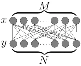
Figure 2: A restricted Boltzmann machine: M is the number of binary observable units x

and N is the number of binary hidden units y. The learning model is p(x,y|a) ∝

exp(∑M

i=1∑Nj=1ai jxiyj), where ai j is a parameter between xiand yj.

Therefore, our aim in this paper is to obtainλandθ.

To assist in achieving this aim, we use the desingularization in algebraic geometry (Watanabe, 2009). It is, however, a new problem, even in mathematics, to obtain the desingularization of Kullback functions, since the singularities of these functions are very complicated and as such most of them have not yet been investigated (Appendix A). We, therefore, need a new method of eigenvalue analysis and a recursive blowing up process.

3. Restricted Boltzmann Machine

From now on, for simplicity, we denote

{{n}}=

0, if n=0 mod 2,

1, if n=1 mod 2, {{(n1,· · ·,nm)}}= ({{n1}},· · ·,{{nm}}),

and we use the notation da instead of∏H_i=1∏H_j=′₁ dai j for a= (ai j). Let 2≤M∈N_{and N∈}N_{. Set}

p(x,y|a) =exp(∑

M

i=1∑Nj=1ai jxiyj)

Z(a) ,

where

Z(a) =

∑

xi=±1,yj=±1,

exp(

M

∑

i=1

N

∑

j=1

ai jxiyj),

Consider a restricted Boltzmann machine

p(x|a) =

∑

yj=±1

p(x,y|a) =∏

N

j=1(∏Mi=1exp(ai jxi) +∏Mi=1exp(−ai jxi))

Z(a)

= {

N

∏

j=1 (

M

∏

i=1

(1+xitanh(ai j)) + M

∏

i=1

(1−xitanh(ai j)))}

∏N

j=1∏Mi=1cosh(ai j)

Z(a)

= ∏

N

j=1∏Mi=1cosh(ai j)

Z(a)

×

N

∏

j=1

(2

∑

0≤p≤M/2i1<

∑

···<i2p

xi1xi2· · ·xi2ptanh(ai1j)tanh(ai2j)· · ·tanh(ai2pj)).

Let B= (bi j) = (tanh(ai j)). Denote BJ=∏Mi=1∏Nj=1b

Ji j

i j and xJ=∏Mi=1x ∑N

j=1Ji j

i , where J= (Ji j) is an M×N matrix with Ji j∈ {0,1}. Then we have

p(x|a) =2

N_∏N

j=1∏Mi=1cosh(ai j)

Z(a)

∑

J:{{∑M

i=1Ji j}}=0for allj

BJxJ.

Let

Z(b) = Z(a)

2N_∏N

j=1∏Mi=1cosh(ai j)

.

Set

I

_{={I= (Ii)∈ {0,1}}M_|{{∑M_i

=1Ii}}=0},and BI=∑J:{{∑M i=1Ji j}}=0

{{∑N j=1Ji j}}=Ii

BJ for I∈

I

_{. Then we have}

p(x|a) = 1 Z(b)_I

∑

_∈I

BIxI

and Z(b) =2NB0.Since∑_0≤i≤M/2

M

2i

= ((1+1)M_{+ (1−1)}M_)/2=2M−1_{, the number of}

ele-ments in

I

_{is 2}M−1_.

Remark 1 Rusakov and Geiger (2005) obtainedλandθfor the following class of Naive Bayesian networks with two hidden states and binary features:

p(x|c,d,t) =t

M

∏

i=1

c(_i1+xi)/2(1−ci)(1−xi)/2+ (1−t) N

∏

i=1

d_i(1+xi)/2(1−di)(1−xi)/2. where x∈ {1,−1}M_{, c={c}

i}Mi=1∈RM, d ={di}Mi=1∈RM and 0≤t≤1. Our models with one

hidden unit (N=1) are obtained by setting t=1/2, tanh(ai) =2ci−1 and di=−ci. The relation

di=−cicreates a parameter space different from that of our models. Assume that the true distribution is p(x|a∗_{)with a}∗_{= (a}∗

i j)and set B∗=b∗= (b∗i j) = (tanh(a∗i j)). Then the Kullback function K(a)is

∑

xi=±1

p(x|a∗)(log p(x|a∗)−log p(x|a)) =

∑

xi=±1

p(x|a∗) ∞

∑

k=2 (−1)k

k (

p(x|a) p(x|a∗₎−1)

k

=

∑

xi=±1

(p(x|a)−p(x|a∗))2 p(x|a∗₎ (1+

∞

∑

k=1 (−1)k

k+2(

p(x|a) p(x|a∗₎−1)

Lemma 1 Watanabe, 2001c If analytic functions K1, K2 satisfy γ1|K2| ≤ |K1| ≤γ2|K2|for some positive constantsγ1andγ2, then the maximum pole and its order ofR|K1|zdw are those ofR|K2|zdw.

By Lemma 1, since we consider a neighborhood of _pp₍(_xx_||_aa∗)₎ =1, we only need to obtain the maximum pole of J(z) =RΨ_z

0db, where

Ψ0=

∑

xi=±1

(p(x|a)−p(x|a∗))2=

∑

xi=±1

(∑I∈IB

I_xI

Z(b) −

∑I∈IB∗IxI Z(b∗) )

2

=

∑

xi=±1 (

∑

I∈I

BI Z(b)−

B∗I Z(b∗)

xI)2₌₂M

∑

I∈I

BI Z(b)−

B∗I Z(b∗)

2

.

By Lemma 1 again, we can replaceΨ0by

Ψ=

∑

I∈{0,1}M

22N( B

I

Z(b)− B∗I Z(b∗₎)

2₌

∑

I∈{0,1}M

(B

I

B0− B∗I B∗0)

2_{. (3)}

4. Main Results

Consider the zeta function J(z) =R

VΨzdb, where V is a sufficiently small neighborhood of a∗. From the eigenvalue analysis method, we obtain the following theorem.

Theorem 2 The average stochastic complexity F(n) in Eq. (1) and the generalization error G(n) in Eq. (2) are given by using the following maximum pole−λof J(z)and its orderθ.

(Case 1): If M=2 thenλ=1/2 andθ=

2, if N=1,b∗=0 1, otherwise.

(Case 2): If M=3 thenλ=

   

  

3/4, if N=1,b∗=0 1/2, if N=1,b∗6=0,∏3

i=1b∗i1=0 3/2, if N=1,∏3

i=1b∗i16=0 3/2, if N≥2,

andθ=

   

  

3, if N=2,b∗=0,

2, if N=2,b∗_6=0,b∗

i0j=b

∗

i1j=0 for 1≤ j≤N,

2, if N=2,b∗_i0j0b_i∗_1j06=0,bi2j0 =b

∗

i j=0 for 1≤i≤3,1≤ j≤N,j6= j0, 1, otherwise,

where

i0,i1,i2∈ {1,2,3}are different from each other and 1≤ j0≤N.

For its proof, we use the eigenvalues and the eigenvectors of the matrix Cj = (cI,I ′

j ) where

bI_j=∏M_i=1bIi

i j, and c I,I′

j =bI

′′

j with{{I′+I′′}}=I, for I,I′,I′′∈

I

. Its proof appears in Appendix B. We obtainλandθin Eqs. (1) and (2) for M>N using a recursive blowing up.

Theorem 3 Assume that M>N and a∗=0. The average stochastic complexity F(n)in Eq. (1) and the generalization error G(n)in Eq. (2) are given by using the maximum pole−λ=−MN

4 of J(z)and its orderθ=

1, if M>N+1,

M, if M=N+1.

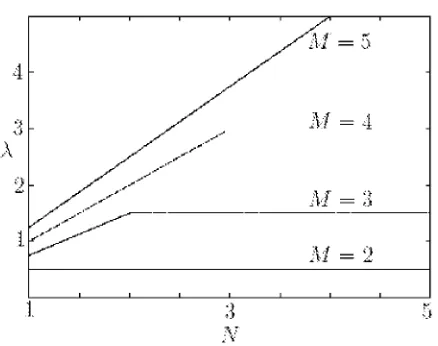
Figure 3: The curve ofλalong the y-axis and N along the x-axis, when M=2,3,4,5 and a∗=0.

Theorem 4 Let(a1 j,a2 j,· · ·,aM j)6=0 for j=1, . . . ,N0 and(a1 j,a2 j,· · ·,aM j) =0 for j=N0+

1, . . . ,N in V , where V is a sufficiently small neighborhood of a∗. Then we have

M(N−N0)

4 ≤λ≤

M(N−N0)

4 +

MN0

2 , if M>N−N0

M(M−1)

4 +

MN0

2 ≤λ≤

2N0+(M−1)(M−2)

4 +

MN0

2

<MN0 2 +

M(N−N0) 4

, if M≤N−N0.

The proofs for these two theorems appear in Appendix C.

5. Conclusion

In this paper, we obtain the generalization error of restricted Boltzmann machines asymptotically (Fig. 3).

We use a new method of eigenvalue analysis and a recursive blowing up in algebraic geometry and show that these are effective for solving the problem in learning theory.

We have not used the eigenvalue analysis method where M >N, which is usually the case in

applications. Eigenvalue analysis seems to be necessary for solving the behavior of the restricted Boltzmann machine model’s generalization error for M≤N.

In this paper, we clarify the generalization error for (i) M =3 (Theorem 2) and (ii) M >N, a∗=0 (Theorem 3) explicitly and give new bounds for the generalization error of the other types (Theorem 4). The case (i) shows thatλis independent of a∗for M−1=2≤N, and so implies that

we need more careful consideration for obtaining the exact valuesλfor the case of Theorem 4. Our future research aims to improve our methods, and to apply them to the case of Theorem 4 and to obtain the generalization error of the general Boltzmann machine, which is also known as the Bayesian network, the graphical model and the spin model, as such models are widely used in many fields. We believe that extending our results would provide a mathematical foundation for the analysis of various graphical models.

The application of our results is as follows. The results of this paper introduce a mathematical measure of preciseness for numerical calculations such as the Markov Chain Monte Carlo. Using the Markov Chain Monte Carlo (MCMC) method, estimated values for marginal likelihoods had previously been calculated for hyper-parameter estimations and model selection methods of com-plex learning models, but the theoretical values were not known. The theoretical values of marginal likelihoods have been given in this paper. This enables us to construct a mathematical foundation for analyzing and developing the precision of the MCMC method (Nagata and Watanabe, 2005). More-over, Nagata and Watanabe (2007) studied the setting of temperatures for the exchange MCMC method and proved the mathematical relation between the symmetrized Kullback function and the exchange ratio, from which an optimal setting of temperatures could be devised. Our theoretical results will be helpful in these numerical experiments. Furthermore, these values have been com-pared with those of the generalization error of a localized Bayes estimation (Takamatsu, Nakajima, and Watanabe, 2005).

Acknowledgments

This research was supported by the Ministry of Education, Science, Sports and Culture in Japan, Grant-in-Aid for Scientific Research 18079007.

Appendix A. Hironaka’s Theorem

We introduce Hironaka’s Theorem about the desingularization.

Theorem 5 [Desingularization (Fig. 4)] (Hironaka, 1964)

Let f be a real analytic function in a neighborhood of w= (w1,· · ·,wd)∈Rd with f(w) =0.

There exist an open set V ∋w, a real analytic manifold U , and a proper analytic map µ from U to V such that

(1) µ : U−

E

_→V−f−1_{(0)is an isomorphism, where}

E

_=µ−1_(f−1_(0)),

(2) for each u∈U , there is a local analytic coordinate system (u1,· · ·,un) such that f(µ(u)) =

±us1 1u

s2

2 · · ·usnn, where s1,· · ·,snare non-negative integers.

Applying Hironaka’s theorem to the Kullback function K(w), for each w∈K−1(0)∩W , we

have a proper analytic map µwfrom an analytic manifold Uw to a neighborhood Vw of w satisfying Hironaka’s Theorem (1) and (2). Then the local integration on Vwof the zeta function J(z)of the learning model is

Jw(z) =

Z

Vw

K(w)zψ(w)dw

= Z

Uw

∑

u

(u2s1 1 u

2s2 2 · · ·u

2sd

d )

z_ψ(µ

w(u))|µ′w(u)|du. (4)

Therefore, the poles of Jw(z)can be obtained. For example, the function

Z

U0 (u2s1

1 u 2s2 2 · · ·u

2sd

d )zu

t1 1u

t2 1· · ·u

td

1du

has the poles−(t1+1)/(2s1),· · ·,−(td+1)/(2sd), where U0 is a small neighborhood of 0. For

Figure 4: Hironaka’s Theorem: This is the picture of a desingularization µ of f :

E

_{maps to f}−1_(0). U−

E

_{is isomorphic to V −f}−1_{(0) by µ, where V is a small neighborhood of w with}

f(w) =0.

Jw(z) =R_VwK(w)zψ(w)dw has no poles. It is known that µ of an arbitrary polynomial in Hironaka’s Theorem can be obtained by using a blowing up process. Note that the exponents in the integral are 2siinstead of sias shown in Eq. (4), since the Kullback function is positive.

In spite of such results, it is still difficult to obtain the generalization error mainly for the follow-ing two reasons. (a) The desfollow-ingularization of any polynomial is in general very difficult, although it is known to be a finite process. Furthermore, most of the Kullback functions of non-regular statistical models are degenerate (overR_{) with respect to their Newton polyhedrons, which is the}

condition for using a toric resolution (Fulton, 1993; Watanabe, Hagiwara, Akaho, Motomura, Fuku-mizu, Okada, and Aoyagi, 2005). Also, points in the singularity set{K=∂K/∂w=0}of Kullback functions K(w)are not isolated, and Kullback functions are not simple polynomials, as their num-ber of variables and numnum-ber of terms grow with parameters, for example, M and N in Eq. (3). It is therefore, a new problem, even in mathematics, to obtain desingularizations of such Kullback functions, since their singularities are very complicated and as such most of them have not yet been investigated. (b) Since our main purpose is to obtain the maximum pole, obtaining a desingulariza-tion is not enough. We need techniques for choosing the maximum one from all poles. However, to the best of our knowledge, no theorems for such a purpose have been developed.

We give below Lemmas 2 and 3 in (Aoyagi and Watanabe, 2005b), as they are frequently used

in this paper. Define the norm of a matrix C= (ci j)bykCk=

q

∑i,j|ci j|2.

Lemma 6 (Aoyagi and Watanabe, 2005b) Let U be a neighborhood of w0 ∈Rd, C(w) be an analytic H×H′ matrix function from U ,ψ(w)be a C∞function from U with compact support, and

P and Q be any regular H×H and H′×H′ matrices, respectively. Then the maximum pole of

R

UkC(w)k2zψ(w)dw and its order are those of

R

UkPC(w)Qk2zψ(w)dw.

Lemma 7 Assume that p(x|a) = ∏

N j=1Wj(x,a) ∑x∏Nj=1Wj(x,a)

for x∈X . Then the maximum pole ofR

U{∑x∈X(p(x|a)−

p(x|a∗))2_}z_{ψ(w)da and its order are those of}

Z

U

{

∑

x,x′_∈X

(

N

∑

j

(logWj(x,a)−logWj(x,a∗)−logWj(x′,a) +logWj(x′,a∗))}2ψ(w)dw.

Consider the ideal I generated by p(x|a)−p(x|a∗_{)for x∈X .}

Then I is generated by ∏

N j=1Wj(x,a) ∏N

j=1Wj(x,a∗)

− ∑x∏Nj=1Wj(x,a)

∑x∏Nj=1Wj(x,a∗), and so by

∏N j=1Wj(x,a) ∏N

j=1Wj(x,a∗)−

∏N

j=1Wj(x′,a) ∏N

j=1Wj(x′,a∗)

for

x,x′∈X .

Since|x−1|/2≤ |log x| ≤2|x−1|for|x−1|<1/2, we have

∑

x,x′_∈X

( ∏

N

j=1Wj(x,a)

∏N

j=1Wj(x,a∗)

∏N

j=1Wj(x′,a∗)

∏N

j=1Wj(x′,a)

−1)2/4

≤

∑

x,x′_∈X

(

N

∑

j

(log(Wj(x,a))−log(Wj(x,a∗)) +log(Wj(x′,a∗))−log(Wj(x′,a))))2

≤

∑

x,x′_∈X

( ∏

N

j=1Wi(x,a)

∏N

j=1Wj(x,a∗)

∏N

j=1Wj(x′,a∗)

∏N

j=1Wj(x′,a)

−1)24

Q.E.D.

Appendix B. Eigenvalue Analysis

The purpose of eigenvalue analysis is to simplify the blowing up process.

Hierarchical learning machines often have Kullback functions involving a matrix product such as K(w) =kD1D2· · ·DNk2, where Diis a parameter matrix. Therefore, analyzing the eigenvalues of these matrices and applying Lemma 6 sometimes results in an easier function to handle. For exam-ple, the restricted Boltzmann machine has a Kullback function k_B˜_Nk2 _{= k 0 E}

CN· · ·C2C1(1,0, . . . ,0)tk2, where E is the identity matrix (t denotes the transpose). Theorem 9

(4) below shows that analyzing the eigenvalues of CNmakes an easier functionkR ˜BNk2to blow up, where R is a certain regular matrix. This is the main point of this method.

Let I,I′,I′′∈

I

_{. We set B}I

N=BI, bIj=∏Mi=1b

Ii

i j, and

BN = (BIN) = (B

(0,...,0)

N ,B

(1,1,0,...,0)

N ,B

(1,0,1,0,...,0)

N , . . .).

We now have BI_N=∑{{I′_+I′′_}}=IbI ′′

NBI

′ N−1.

For convenience, we denote the “(I,I′)th” element of a 2M−1×2M−1matrix C by cI,I′. Now consider the eigenvalues of the matrix CN= (cI,I

′

N )where c I,I′

N =bI

′′

N with{{I′+I′′}}=I.

Note that BN=CNBN−1.

Letℓ= (ℓ1, . . . , ℓ2M−1) = (ℓ_I)∈ {−1,1}2

M−1

withℓ_(0,...,0)=1.ℓis an eigenvector, if and only if

∑

I′_∈I

cI_N,I′ℓI′=ℓ_I

∑

I′_∈I

c(_N0,...,0),I′ℓI′ =ℓ_I

∑

I′_∈I

bI_N′ℓI′, for all I∈

I

.

That is,

ℓis an eigenvector ⇐⇒ if{{I+I′}}=I′′({{I+I′+I′′}}=0) thenℓI′′=ℓ_Iℓ_I′ (ℓ_Iℓ_I′ℓ_I′′=1).

Theorem 8 Let K1⊂ {2, . . . ,M}. SetℓI=

−1, if #{i∈K1: Ii=1}is odd,

1, otherwise. Thenℓ= (ℓI)is

an eigenvector of CNand its eigenvalue is

∑

I∈I ℓIbIN=

∏M

i=1(1+xibi) +∏Mi=1(1−xibi)

2 ,where xi=−1 if i∈K1,and xi=1 if i6∈K1.

Note that∑I∈IℓIbNI >0 since bi=tanh(ai).

(Proof)

Assume that {{I′_+I′′_+I′′′_{}}=0. If all #{i∈K}

1: Ii′=1}, #{i∈K1: Ii′′=1}and #{i∈K1: I_i′′′=1}are even, thenℓI′ℓ_I′′ℓ_I′′′=1.

If #{i∈K1: Ii′=1}is odd, then #{i∈K1: Ii′′=1}or #{i∈K1: Ii′′′=1}is odd, since{{I′+

I′′+I′′′}}=0.

If #{i∈K1: Ii′=1}and #{i∈K1: Ii′′=1}are odd, then #{i∈K1: Ii′′′=1}is even andℓI′ℓ_I′′ℓ_I′′′= 1 since{{I′_+I′′_+I′′′_}}=0.

Q.E.D.

We have 2M−1eigenvectorsℓ. Moreover, they are orthogonal to each other, since the eigenvec-tors of a symmetric matrix are orthogonal. These eigenveceigenvec-torsℓ’s, therefore, span the whole space

R2M−1_.

Set 1= (1, . . . ,1)t _∈Z2M−1−1 _{(t denotes the transpose). Let D= (D}I,I′_{)be a symmetric matrix} formed by arranging the eigenvectorsℓ’s such that D=

1 1t 1 D′

and DD=2M−1E, where E is

the identity matrix and DI,I′ is “(I,I′)th” element of D.

Since DD=

2M−1 1tD′

1+D′1 11t+D′D′

=2M−1E, we have D′1=−1.

Let C_N′ =DCND/2M−1=DCND−1=



   

s0_N 0 0 · · · 0 0 s1_N 0 · · · 0

..

. ... ... ... ... 0 0 0 · · · s2_NM−1−1



   

.

We use si_N or sI_N(I∈

I

_{), depending on the situation.}

Since CN=D−1C_N′ D, we have b_N{{I+K}}=∑J∈IDI,JsJ_NDJ,K/2M−1.

B.1 Example

Let M=4.

D=



          

1 1 1 1 1 1 1 1

1 −1 −1 −1 1 1 1 −1

1 −1 1 1 −1 −1 1 −1

1 −1 1 −1 −1 1 −1 1 1 1 −1 −1 −1 −1 1 1

1 1 −1 1 −1 1 −1 −1

1 1 1 −1 1 −1 −1 −1

1 −1 −1 1 1 −1 −1 1



          

and the eigenvalues

s0_N = 1+b1Nb2N+b1Nb3N+b1Nb4N+b2Nb3N+b2Nb4N+b3Nb4N+b1Nb2Nb3Nb4N, s1_N = 1+b2Nb3N+b2Nb4N+b3Nb4N−b1N(b2N+b3N+b4N+b2Nb3Nb4N),

s2_N = 1+b1Nb3N+b1Nb4N+b3Nb4N−b2N(b1N+b3N+b4N+b1Nb3Nb4N), s3_N = 1+b1Nb3N+b2Nb4N+b1Nb2Nb3Nb4N−(b1N+b3N)(b2N+b4N), s4_N = 1+b1Nb2N+b3Nb4N+b1Nb2Nb3Nb4N−(b1N+b2N)(b3N+b4N), s5_N = 1+b1Nb2N+b1Nb4N+b2Nb4N−b3N(b1N+b2N+b4N+b1Nb2Nb4N), s6_N = 1+b1Nb2N+b1Nb3N+b2Nb3N−b4N(b1N+b2N+b3N+b1Nb2Nb3N), s7_N = 1+b1Nb4N+b2Nb3N+b1Nb2Nb3Nb4N−(b1N+b4N)(b2N+b3N).

Theorem 9 Let H=2M−1−1.

(1) Let di j=

    

   

1, if i=1 or j=1,

DI,J, if I= _{(1, 0, . . . , 0, 1}i_{, 0, . . . , 0)}

and J= _{(1, 0, . . . , 0, 1}j_{, 0, . . . , 0).}

Then DI,J =∏i,j:Ii=1,Jj=1di j for all I,J∈

I

.

(2) BN=CNBN−1=CN· · ·C2B1=DCN′ · · ·C2′D−1B1=

DC_N′ · · ·C₁′1 2M−1 . (3) We have 2M−1D′−1=D′−11t.

(4) Let ˜B1= (BI₁)I6=0, ˜BN= (BIN)I6=0and

S=− 1

H+1



 

∏N j=1s∗

1

j−∏Nj=1s∗ 0

j

.. .

∏N

j=1s∗Hj −∏Nj=1s∗0j



  ∏

N

j=2s1j−∏Nj=2s0j · · · ∏Nj=2sHj −∏Nj=2s0j

+B∗0_N∏N_j=2s0_j



 

1 · · · 1

..

. ... ...

1 · · · 1



 +B

∗0

N



   

∏N

j=2s1j 0 0 · · · 0 0 ∏N_j=2s2

j 0 · · · 0

..

. ... ... ...

0 0 0 · · · ∏N

j=2sHj



   

.

We have

(det S)D′−1S−1D′−12M−1(_B˜_NB∗0

= (det S)_B˜_1−(B∗0

N)H−1(1 D′)



 

∏N

j=1s∗0j∏i=6 0∏Nj=2sij

.. .

∏N j=1s∗

H

j ∏i6=H∏Nj=2sij



 .

(5) The corresponding element to I of (1 D′)



 

∏i6=0∏Nj=2sij

.. .

∏i6=H∏Nj=2sij





 consists of monomials

cJ∏Mi=1∏Nj=2b

Ji j

i j, where cJ∈R, 0≤Ji j∈Zand{{∑ N

j=1Ji j}}=Ii. (Proof)

(1) Fix K1⊂ {2, . . . ,M}.

Consider the eigenvectorℓdefined by using K1.

Set d₁′ =1 and d_i′=ℓI for I= _{(1, 0, . . . , 0, 1}i_{, 0, . . . , 0)} , i≥2. SinceℓI=∏i∈K1:Ii=1(−1) =∏i:Ii=1d

′

i and D is symmetric, we have statement (1). (2) is obvious.

(3) Since DD=

2M−1 1tD′

1+D′1 11t+D′D′

=2M−1E, we have D′D′=2M−1E′−11t and D′(D′−

11t) =2M−1E′−11t−D′11t=2M−1E′−11t+11t=2M−1E′, where E′is the identity matrix. (4)

2M−1(_B˜_NB∗0

N−B˜∗NB0N) =2M−1 −B˜∗N B∗0NE

BN

= −_B˜∗

N B∗0NE

D



   

∏N

j=2s0j 0 0 · · · 0 0 ∏N_j=2s1

j 0 · · · 0 ..

. ... ... ...

0 0 0 · · · ∏N

j=2sHj



   

DB1

= (−_B˜∗

N 1 1t

+B∗0_N 1 D′ )



   

∏N

j=2s0j 0 0 · · · 0 0 ∏N_j=2s1_j 0 · · · 0

..

. ... ... ...

0 0 0 · · · ∏N

j=2sHj



   

DB1

= (− 1 D

′

H+1



   

∏N j=1s∗

0

j

∏N j=1s∗1j

.. .

∏N j=1s∗

H j



   

1 1t +B∗0_N 1 D′ )



   

∏N

j=2s0j 0 0 · · · 0 0 ∏N_j=2s1_j 0 · · · 0

..

. ... ... ...

0 0 0 · · · ∏N

j=2sHj



   

= 1 D′ (− 1

H+1

     ∏N j=1s∗0j

∏N j=1s∗1j

.. .

∏N j=1s∗Hj

     ∏N

j=2s0j · · · ∏Nj=2sHj

+B∗0_N

     ∏N

j=2s0j 0 0 · · · 0 0 ∏N_j=2s1_j 0 · · · 0

..

. ... ... ...

0 0 0 · · · ∏N

j=2sHj

     )( 1 1 + 1t D′ ˜ B1)

=D′(−T0



 

∏N

j=1s∗1j−∏Nj=1s∗0j ..

.

∏N

j=1s∗Hj −∏Nj=1s∗0j



 +B

∗0 N    ∏N

j=2s1j−∏Nj=2s0j ..

.

∏N

j=2sHj −∏Nj=2s0j



 ) +D

′_SD′_B1,˜

where T0=∏

N

j=2s0j+···+∏ N

j=2sHj

H+1 .

Also we have S−_i 1

1j1= (det S)

−1_×

      

(B∗0N)H−2

H+1 ∑

H

i2=0,i26=i1(∏

N j=1s∗

i1

j +H∏Nj=1s∗

i2

j)∏0≤i≤H,i6=i1,i2∏

N

j=2sij, if i1= j1,

(B∗0

N)H−2

H+1 ∑0≤i2≤H,i26=i1,j1(∏

N j=1s∗

i1

j −∏Nj=1s∗

i2

j)∏0≤i≤H,i6=i1,i2∏

N j=2sij

−(B∗0N)H−2

H+1 (H∏

N j=1s∗

i1

j +∏Nj=1s∗

j1

j )∏0≤i≤H,i6=i1,j1∏

N

j=2sij, if i16= j1

and det S= (B∗0_N)H−1_∑H i2=0∏

N j=1s∗

i2

j ∏i6=i2∏

N j=2sij. Let s=



 

∏N

j=1s∗0j∏i=6 0∏Nj=2sij ..

.

∏N

j=1s∗Hj ∏i=6 H∏Nj=2sij





and ˜s= 

 

∏N

j=1s∗1j∏i=6 1∏Nj=2sij ..

.

∏N

j=1s∗Hj ∏i=6 H∏Nj=2sij



 .

Since(det S)S−1_(−T0



 

∏N j=1s∗

1

j−∏Nj=1s∗ 0

j ..

.

∏N

j=1s∗Hj −∏Nj=1s∗0j



 +B

∗0 N    ∏N

j=2s1j−∏Nj=2s0j ..

.

∏N

j=2sHj −∏Nj=2s0j



 )

= (B∗0_N)H−1_{∑H i2=0∏

N j=1s∗

i2

j ∏i6=i2∏

N

j=2sij1−(H+1)



 

∏N

j=1s∗1j∏i=6 1∏Nj=2sij ..

.

∏N j=1s∗

H

j ∏i6=H∏Nj=2sij



 },

we have

D′−1S−1D′−12M−1(B˜NB∗0N−B˜∗NB0N)

= (det S)_B1˜ _−(B∗0

N)H−1

H

∑

i2=0

N

∏

j=1 s∗i2

j

∏

i6=i2

N

∏

j=2

si_j1−(H+1)(B∗0_N)H−1D′−1˜s

= (det S)B1˜ −(B∗0_N)H−1

H

∑

i2=0

N

∏

j=1 s∗i2

j

∏

i6=i2

N

∏

j=2

si_j1−(B∗0_N)H−1(D′−11t)˜s

= (det S)_B˜_1−(B∗0

N)H−1

N

∏

j=1 s∗0_j

∏

i6=0

N

∏

j=2

si_j1−(B∗0_N)H−1_D′_˜s

= (det S)_B˜_1−(B∗0

by using (3).

(5) Since b{{_j I+K}}=∑J∈IDI,JsJ_jDJ,K/2M−1, we have for I′∈

I

,

∑

J∈I

DI,Js{{_j J+I′}}DJ,K=DI,I′DI′,K

∑

J∈I

DI,{{J+I′}}s{{_j J+I′}}D{{J+I′}},K

= 2M−1DI,I′DI′,Kb{{_j I+K}},

by using (1).

Let I0= (0, . . . ,0),I1= (1,1,0, . . . ,0),I2= (1,0,1,0, . . . ,0), . . ..

The fact that

D     

∏i6=0∏Nj=2sij

∏i6=1∏Nj=2sij .. .

∏i6=H∏Nj=2sij

     = −D     

∏i6=0∏Nj=2sij 0 0 · · · 0 0 ∏_i6=1∏N_j=2si

j 0 · · · 0 ..

. ... ... ... ...

0 0 0 · · · ∏_i6=H∏N j=2sij



   

D−12M−1

     1 0 .. . 0      = −            N

∏

j=206=

∏

I′_∈I D      

s{{I0+I′}}

j 0 0 · · · 0

0 s{{I1+I′}}

j 0 · · · 0

..

. ... ... ... ... 0 0 0 · · · s{{IH+I′}}

j      

D−1

          

2M−1

     1 0 .. . 0      ,

and∑_J∈IDI,Js {{J+I′}}

j DJ,K=2M−1DI,I

′

DI′,K_b{{I+K}}

j yields statement (5).

Q.E.D. Proof of Theorem 2

By Theorem 9 (4) and Lemma 6, we only need to consider the maximum pole of J(z) =

R

kΨ′_k2z_db,whereΨ′_{= (det S)B˜}

1−(B∗0N)H−1(1 D′)



 

∏N

j=1s∗0j∏i=6 0∏Nj=2sij ..

.

∏N j=1s∗

H

j ∏i6=H∏Nj=2sij



 .

(Case 1): The fact that B11=∑N_k=1b1kb2k+· · · provides Case 1. (Case 2): Assume that M=3.

We have D′=





1 −1 −1

−1 1 −1

−1 −1 1

 ,       

s0_j =1+b1 jb2 j+b1 jb3 j+b2 jb3 j, s1_j =1+b1 jb2 j−b1 jb3 j−b2 jb3 j, s2_j =1−b1 jb2 j+b1 jb3 j−b2 jb3 j, s3_j =1−b1 jb2 j−b1 jb3 j+b2 jb3 j,

andΨ′= (det S)





b11b21 b11b31 b21b31



−∏3_i=0∏N_j=2si_j(B∗0_N)2(1,D′)      ∏N j=1s∗

0

j/∏Nj=2s0j

∏N j=1s∗

1

j/∏Nj=2s1j

∏N

j=1s∗2j/∏Nj=2s2j

∏N

j=1s∗3j/∏Nj=2s3j

Let N=1. The fact thatΨ′=4(B∗_N0)2_{B1˜ −4(B}∗0

N)2





b∗₁₁b∗₂₁ b∗₁₁b∗₃₁ b∗₂₁b∗₃₁



yields the statement for N=1.

Assume that N ≥2, b∗6=0 and b∗₁₁=6 0,b∗₂₁6=0,b∗₃₁6=0. Set b′₂₁=b11b21, b′31=b11b31and b′₁₁=b21b31=b′21b′31/b211. Then

Ψ′_{= (det S)}





b′₂₁ b′₃₁ b′₁₁



−

3

∏

i=0

N

∏

j=2

si_j(B∗0_N)2(1,D′)

     ∏N

j=1s∗0j/∏Nj=2s0j

∏N

j=1s∗1j/∏Nj=2s1j

∏N

j=1s∗2j/∏Nj=2s2j

∏N j=1s∗

3

j/∏Nj=2s3j



   

and its maximum pole is 3/2 and its order is 1.

Assume that N ≥ 2, b∗ 6=0, b∗₁₁ 6= 0 and ∏3_i=1b∗_{i j} =0 for all j. Let ψ =

  ψ1 ψ2 ψ3   =

(1,D′₎

     ∏N j=1s∗

0

j/∏Nj=2s0j

∏N j=1s∗

1

j/∏Nj=2s1j

∏N

j=1s∗2j/∏Nj=2s2j

∏N

j=1s∗3j/∏Nj=2s3j



   

.By setting

b′₂₁ b′₃₁

= (det S)

b11b21 b11b31

−∏3

i=0∏Nj=2sij(B∗

0

N)2

1 1 −1 −1 1 −1 1 −1

     ∏N j=1s∗

0

j/∏Nj=2s0j

∏N

j=1s∗1j/∏Nj=2s1j

∏N

j=1s∗2j/∏Nj=2s2j

∏N

j=1s∗3j/∏Nj=2s3j

     and

Ψ′′₌

  Ψ′′ 1 Ψ′′ 2 Ψ′′ 3  =   

b′₂₁ b′₃₁

(∏3

i=0∏Nj=2sij(B∗

0

N)2)2ψ1ψ2

b211det S

−(B∗0_N)2_∏3

i=0∏Nj=2sijψ3



 ,

and by using Lemma 6, we need the maximum pole ofR

kΨ′′_k2z_{db. Ψ}′′_{is singular in the following}

cases: (i) b∗₁₁b∗₂₁=b_{2 j}∗ =b∗_{3 j} =0 for all j, (ii) b∗₁₁b∗₂₁6=0, b∗_{1 j}=b∗_{2 j}=b∗_{3 j}=0 for all j, since we have _∂∂ψ_b

j|b

∗

=−(1,D′)



  

s∗0₁/s∗0_j 0 0 0

0 s∗1₁/s∗1

j 0 0

0 0 s∗2₁/s∗2_j 0 0 0 0 s∗3₁/s∗3_j

       

b∗_{2 j}+b∗_{3 j} b∗_{1 j}+b∗_{3 j} b∗_{1 j}+b∗_{2 j} b∗_{2 j}−b∗_{3 j} b∗_{1 j}−b∗_{3 j} −b∗

1 j−b∗2 j −b∗_{2 j}+b∗_{3 j} −b∗_{1 j}−b∗_{3 j} b∗_{1 j}−b∗_{2 j} −b∗

2 j−b∗3 j −b∗1 j+b∗3 j −b∗1 j+b∗2 j



  

.If

Ψ′′_{is not singular, its maximum pole is 3/2 and its order is 1. Assume that Ψ}′′_{is singular that is,}

(i) b∗₁₁b∗₂₁=b_{2 j}∗ =b∗_{3 j}=0 for all j and (ii) b∗₁₁b∗₂₁6=0,b∗_{1 j}=b∗_{2 j}=b∗_{3 j}=0 for all j. Construct the blow-up ofΨ′′along the submanifold{b3 j=0,2≤ j≤N}. Let b32=u and b3 j=ub′3 jfor j≥2.

In the case (i), the coefficient of b2 j0 is around 4ub1 j0∑

N

j=2b1 jb′3 j(1/b112 −1) +4ub′3 j0(1−b 2 1 j0),

since∏_i6=0∏N_j=2si_j ∼=∏Nj=2(1−b1 jb2 j−ub1 jb′3 j−ub2 jb′3 j+2ub21 jb2 jb′3 j)∼=1+∑Nj=2(−b1 jb2 j− ub1 jb′_{3 j} − ub2 jb′_{3 j} + 2ub2_{1 j}b2 jb′_{3 j}) + ∑j6=j′ub1 jb_{1 j}′b2 jb′_{3 j}′, ∏i=0∏Nj=2sijψ1 ∼= − 4∑N_j=2b1 jb2 j, ∏i=0∏Nj=2sijψ2 ∼= −4u∑Nj=2b1 jb′3 j, and ∏i=0∏Nj=2sijψ3 ∼=

4∑N_j=2(−ub2 jb3 j′ +2ub21 jb2 jb′3 j) +4∑j6=j′ub_{1 j}b_{1 j}′b_{2 j}b′_{3 j}′. If 4ub1 j0∑

N

4ub′_{3 j0}(1−b2_{1 j0}) =0 for all j0 then b′3 j0 =0 for all j0 since|b1 j|<1. It contradicts b

′

32=1. So ((∏

3

i=0∏Nj=2sij(B∗

0

N)2)2ψ1ψ2

b2 11det S

−(B∗0_N)2_∏3

i=0∏Nj=2sijψ3)/u is smooth.

In the case (ii), the coefficient b2 j0 is around 4u(1−b

∗ 21

2_)b′

3 j0 since s

∗0

1∏i6=0∏Nj=2sij ∼=4(1+

b∗₁₁b∗₂₁)∏N_j=2(1−ub2 jb′_{3 j})=∼4(1+b∗₁₁b∗₂₁)(1−u∑N_j=2b2 jb′_{3 j}),(1+b∗₁₁b∗₂₁)∏i=0∏Nj=2sijψ1∼=4b∗₁₁b∗₂₁,

∏i=0∏Nj=2sijψ2 ∼= −4ub∗₁₁b∗₂₁∑Nj=2b2 jb3 j′ , and ∏i=0∏Nj=2sijψ3 ∼= −4u∑Nj=2b2 jb′3 j. So ((∏

3

i=0∏Nj=2sij(B∗0N)2)2ψ1ψ2

b2 11det S

−(B∗0_N)2_∏3

i=0∏Nj=2sijψ3)/u is smooth. We haveΨ′′=





b′₂₁ b′₃₁ ub′₂₂



,for a variable b′₂₂for both cases (i) and (ii) and we have the statement

for N≥2, b∗6=0, b∗₁₁6=0 and∏3_i=1b∗_{i j}=0 for all j. Let N≥2 and b∗=0.

Construct the blow-up ofΨ′along the submanifold{bi j=0,1≤i≤M,1≤ j≤N}. Let b11=u and bi j=ub′i j for(i,j)6= (1,1).

We have Ψ′′=u2(det S)





b′₂₁ b′₃₁ b′₂₁b′₃₁



+4u2 

 ∑N

k=2b′1kb′2k+u2f1

∑N

k=2b′1kb′3k+u2f2

∑N

k=2b′2kb′3k+u2f3



, where f1, f2 and f3 are

polynomials of b′_{i j}of at least degree two.

By setting

b′′₂₁ b′′₃₁

=

b′₂₁ b′₃₁

+4

∑N

k=2b′1kb′2k+u2f1

∑N

k=2b′1kb′3k+u2f2

/(det S),we have

Ψ′′₌ u2

det S

×





(det S)2_b′′ 21 (det S)2_b′′

31

(b′′₂₁det S−4∑N_k=2b′_1kb′_2k−4u2f1)(b′′31det S−4∑Nk=2b′1kb′3k−4u2f2)





+u2





0 0

4∑N_k=2b_2k′ b′_3k+4u2f3



.

By using Lemma 6 again, the maximum pole ofR

kΨ′′k2z_u3N_{db is that of J(z) =}R

kΨ′′′k2z_u3N_db,

whereΨ′′′=u2





b′′₂₁ b′′₃₁ g1



,and

g1= (

N

∑

k=2

b′_1kb′_2k+u2f1)(

N

∑

k=2

b′_1kb′_3k+u2f2) +

det S 4 (

N

∑

k=2

b′_2kb′_3k+u2f3).

Construct the blow-up of Ψ′′′ along the submanifold {b′′₂₁=0,b′′₃₁ =0,b′_3k =0,2≤k ≤N}. Then we have cases (I) and (II).

(I) Let b′₃₂=v, b′′₂₁=vb′′′₂₁, b′′₃₁=vb′′′₂₁ and b′_3k=vb′′_3k for 3≤k≤N. ThenΨ′′′=u2v





b′′′₂₁ b′′′₃₁ g′₁



,

where g′₁= (∑N