Maximizing Power Loss Reduction in Radial Distribution Systems by
Using Modified Gray Wolf Optimization
Deepa Nataraj
1,*, Rajaji Loganathan
2, Moorthy Veerasamy
3, Venkata Durga Ramarao Reddy
41St. Peter’s Institute of Higher Education and Research, Deemed to be University, Chennai, India 2ARM College of Engineering and Technology, Chennai, India
3Swarnandhra College of Engineering and Technology, Narsapur Bhimavaram, India 4
Vishni Institute of Technology, Bhimavaram, India
Received 22 June 2018; received in revised form 27 December 2018; accepted 30 December 2018
Abstract
This paper presents an optimal Distribution Network Reconfiguration (DNR) framework and solution procedure that employ a novel modified Gray Wolf Optimization (mGWO) algorithm to maximize the power loss reduction in a Distribution System (DS). Distributed Generation (DG) is integrated optimally in the DS to maximize the power loss reduction. DNR is an optimization problem that involves a nonlinear and multimodal function optimized under practical constraints. The mGWO algorithm is employed for ascertaining the optimal switching position when reconfiguring the DS to facilitate the maximum power loss reduction. The position of the gray wolf is updated exponentially from a high value to zero in the search vicinity, providing the perfect balance between intensification and diversification to ascertain the fittest function and exhibiting rapid and steady convergence. The proposed method appears to be a promising optimization tool for electrical utility companies, thereby modifying their operating DS strategy under steady-state conditions. It provides a solution for integrating more DG optimally in the existing distribution network. In this study, IEEE 33-bus and 69-bus DSs are analyzed for maximizing the power loss reduction through reconfiguration, and the integration of DG is exercised in the 33-bus test system alone. The simulation results are examined and compared with those of several recent methods. The numerical results reveal that mGWO outperforms other contestant algorithms.
Keywords: radial distribution system, network reconfiguration, power loss reduction, modified gray wolf optimization, distributed generation
1.
Introduction
In an electrical utility system, a Distribution System (DS) is an extensive part that usually supplies the consumer demand for electricity at an acceptable voltage magnitude. Generally, a DS operates in a radial structure to facilitate efficient protection and coordination schemes that can be re-structured for optimizing the controllable parameter. Distribution Network Reconfiguration (DNR) is the procedure for changing the topology of distribution feeders by changing the open / closed status of sectionalizing and tie switches while satisfying system constraints to satisfy the operator’s objectives. This has been
mathematically devised as an optimization problem subjected to various operational restrictions for ascertaining an optimal radial structure that reduces the power loss and load-balancing index [1-2] or maximizes the benefits under normal operation
conditions [3]. In this context, some metaheuristic algorithms for minimizing power loss and maximizing node voltage magnitude of the DS have been presented, such as the Genetic Algorithm (GA) [4], the ant colony search algorithm [5], evolutionary algorithms [6], the plant growth simulation algorithm [7], the bacterial foraging optimization algorithm [8], and the cuckoo search algorithm [9]. These algorithms competently reconfigure the DS for minimizing power loss, improving the voltage profile of the distribution network. The convergence characteristic of a metaheuristic algorithm is dependent on an appropriate balance between exploration and exploitation behaviors. Therefore, researchers are attempting to tune the control variable of metaheuristic algorithms toward a global optimum, whereas mathematical methods have failed to find a correct solution. For this purpose, either a stochastic technique is incorporated to modify the heuristic operator or a hybrid optimization technique is developed by combining two heuristic tools or knowledge elements, as well as more traditional approaches being employed.
In line with this discussion, Swarnkar adopted graph theory with the conventional ant colony optimization algorithm, modifying the standard algorithm to perform Adaptive Ant Colony Optimization (AACO) [10]. This modified algorithm places feasible individuals in the space and overrides the mesh check. Likewise, in the Improved Adaptive Imperialist Competitive Algorithm (IAICA), a mapping strategy is incorporated, which adapts the imperialist competitive algorithm into a discrete nonlinear optimization problem [11]; the step size of the E. coli of the Modified Bacterial Foraging Optimization Algorithm (MBFOA) varies in each iteration [12]; and in Adaptive Weighted Improved Discrete Particle Swarm Optimization (AWIDPSO), the inertia weight is adaptively varied [13]. Conversely, in Mixed-Integer Hybrid Differential Evolution (MIHDE) [14], common mixed-integer nonlinear programming is embedded in a hybrid differential evolution algorithm. This algorithm performs migration and acceleration operations, which result in upgrades of the exploration tendency of the algorithm in the search space to improve fitness.
An extensive literature survey has revealed that DNR is a complex and nonlinear optimization problem that aims to minimize power loss, load balancing among branches, load balancing among feeders, node voltage deviation, and the number of switching operations either alone or through multiple objectives. Namely, AACO, MBFOA, AWIDPSO, and MIHDEhave been devised solely for minimizing power loss, whereas IAICA was devised to reduce power loss and node voltage deviation separately. Similarly, hybrid particle swarm optimization [15] and the runner-root algorithm [16] have been employed to ascertain the optimal distribution reconfiguration in a multiobjective environment, wherein the norm 2 and max-min methods are incorporated, respectively, to obtain a compromised membership function between the best and worst objective functions. Similarly, AWIDPSO has been used for determining the optimal distribution restructure in a multiobjective scenario wherein the compromised objective function is obtained through a fuzzy membership function [17]. Power loss reduction of the current DS through physical restructuring is known to be possible to a certain level. To reduce the power loss and improve the voltage profile, a capacitor bank can be placed in the existing DS. The capacitor size and location are optimized using the flower pollination algorithm of Abdelaziz [18] and improved harmony algorithm of Ali [19]. Subsequently, Distributed Generation (DG) in the DS is optimized using the ant lion optimization algorithm [20].
GWO uses encircling, hunting, and attacking processes for discovering a superior solution when solving various standard test functions, performing sophisticated engineering, solving unit commitment problems, and dispatching economic loads. The acceleration set (a) of the coefficient vector (A) in the GWO position update equation decreases linearly from a higher value to zero. Equal opportunity is provided to both global and local optima because the trade-off between exploration and exploitation occurs linearly. In this paper, modified GWO (mGWO) is proposed, and this method increases the diversity of global optimum solution for a DNR problem. An exponential function is employed to obtain a trade-off between exploration and exploitation throughout the iterations. Increasing the degree of exploration in comparison to exploitation increases the convergence speed and avoids local minima trapping. When mGWO is used for solving a DNR problem for the first time, it provides practical solutions for IEEE 33 and 69 buses, and the global optimum solution is obtained quickly.
The rest of this paper is organized as follows. Section 2 describes the DNR problem. The mGWO algorithm is proposed in Section 3. The implementation of mGWO is demonstrated in Section 4. The simulation results are presented in Section 5. Finally, the study is concluded in Section 6.
2.
Articulation Of The DNR Problem
2.1. Distribution network model for loss reduction
The power flow in a DS can be computed from the simplified DS model illustrated in Fig. 1 by using a recursive procedure. Active power flows through branch k from bus p to bus q, which is expressed as Eq. (1) and can be conveniently abridged as in Eq. (2).
Fig. 1 Simplified DS model
, ,
p q eff k loss
P P P (1)
where
, ,
q eff p q L
P P P (2)
The current flowing through branch k between buses p and q can be calculated using either Eq. (3) or Eq. (4):
p p
k
p p
P jQ
I V
(3)
p p q q
k
k k
V V
I
R jX
(4)
When computing the power loss in the DS, the voltage at bus q must be calculated. For this purpose, first, Eqs. (3) and (4) are compared. Second, the real and imaginary parts are separated. Third, the real and imaginary parts are squared and summed. Thus, the bus voltage is obtained as
2 22 2 2 2
2
2 * p p
q p p k p k k k
p
P Q
V V P R Q X R X
V
(5)
The power loss in a line segment that connects buses p and q can be determined using Eq. (6).
th
p bus q busth
k k
R jX
p p
V Vqq
p p
P jQ PqjQq
, ,
q L q L
P jQ
k
2 2
, ,
2
, * 2 *
q eff q eff
k loss k k k
q
P Q
P I R R
V (6)
The aggregate power loss of the feeder can then be calculated by summing the losses of all line segments of the feeder, which is given as
2 2 1 , , 2 2 1 * bus bus N N
q eff q eff
Loss k
q k q
P Q P R V
(7)The power loss of a line segment connecting buses p and q after network reconfiguration can be computed as
'2 '2
, ,
' '2
2 '
* q eff q eff *
k k k k
q
P Q
P I R R
V (8)
The aggregate power loss of the feeder can then be determined by summing the losses of all line segments of the feeder, which is given as
'2 '2 1 , , ' 2 ' 2 1 * bus bus N N
q eff q eff
Loss k q k q P Q P R V
(9)The net power loss reduction, in the system, is difference in power loss before, after reconfiguration, and is given as
2 2 ' 2 ' 2
1 1
, , , ,
2 '2
2 1 2 1
* *
bus bus bus bus
N N N N
q eff q eff q eff q eff
Loss k k
q k q k
q q
P Q P Q
P R R
V V
(10)2.2. Power loss reduction due to DG
If DG is optimally located in a week node of the DS using the loss sensitivity factor approach, technical, economic and environmental benefits are obtained. The effect on power loss in the line segment between buses p and q is computed using
2 2
, , 2 2
, 2 * 2 2 , 2
q eff q eff
DG k
k Loss k g g q eff g qeff g
q q
P Q R D
P R P Q P P Q Q
L V V (11)
The net power loss reduction in a DS is the difference between the power loss that occurs in the system without and with DG and is calculated as
1 2 2 , 2 2 1 2 2 bus bus N N DG kLoss g g q eff g qeff g
q k q
R D
P P Q P P Q Q
L V
(12)2.3. Objective functions 2.3.1. Network reconfiguration
The objective function is formulated by taking the difference in the power loss of all line sections of the feeder as well as the network reconfiguration. For this purpose, an appropriate candidate open-switch position, the power loss reduction of a branch segment, is computed and should be maximized; the objective function is defined mathematically as
Loss
2.3.2. DG integration
The objective function for maximizing the net power loss reduction computed using Eq. (12) is expressed as
DG
Loss
Objective function f Maximize P (14)
2.4. Constraints
The node voltage should be between its lower and upper limits:
min q max
;
busV
V
V
q
N
(15)The branch current should be less than or equal to its maximum capacity, as specified by the manufacturer [1]:
max ;
k k br
I I kN (16)
The total size of DG is always less than or equal to the total load and active power loss of the network. The minimum and maximum DG kW ratings are selected as 10 % and 80 % of the entire system’s real power demand, respectively.
, 1 DG
N
g k Load Loss
k
P P P
(17)3.
Modified Gray Wolf Optimization
The basic GWO algorithm, developed by Seyedali Mirjalili, mimics the leadership hierarchy, and hunting mechanism of gray wolves in nature [21]. In their population, gray wolves are categorized as alpha (α), beta (β), delta (δ), or omega (ω); the
alpha is most dominant, whereas deltas and omegas control the rest of the wolves. The critical behavior in GWO is encircling, hunting, and attacking the prey, analytically modeled as an optimization tool for obtaining the optimal solution for any problem. The hunting mechanism of gray wolves is described in the following.
3.1. Encircling
This gray wolf behavior is modeled by
prey wolf
D C X t X t (18)
1
wolf prey
X t X t A D (19)
The vectors “A” and “C” play a crucial role in updating the position of a wolf according to that of the prey [21],
considering a two-dimensional position vector and some of the possible neighbors. These coefficients are determined using Eqs. (20) and (21), where coefficient “a” is decreased linearly from 2 to 0 throughout the iterations.
1
2
A a r a (20)
2
2.
C r (21)
3.2. Hunting
Generally, the alpha wolf, in association with beta and delta wolves, presides over the hunting. To mimic hunting behavior, three of the best candidate solutions are alpha, beta, and delta wolves, which are first considered during the iteration. The other search agents (omega wolves) update their positions according to those of the three best search agents. This can be mathematically modeled as [21]
1
2
3
1
3
X t X t X t
where
1 aplha 1 alpha ; 2 beta 2 beta ; 3 delta 3 delta
X X A D X X A D X X A D (23)
1 ; 2 ; 3
alpha alpha beta beta delta delta
D C X X D C X X D C X X (24)
3.3. Attacking
In this phase, the wolves move in to assault the prey. In the mathematical model indicating the approaching of the victim, coefficient vector “A” plays a vital role and its oscillation range decreases by vector “a.” Moreover, vector “A” has a random value in the interval [−𝑎, 𝑎], where “a” is decreased linearly from 2 to 0 throughout the iterations. At the point where random generations of vector “A” are in the range [−1, 1], the subsequent position of a candidate solution can be anywhere between its present location and the prey’s location. The candidate solution converges if the magnitude of vector “A” satisfies Eq. (25);
alternatively, it diverges from the prey if the magnitude satisfies Eq. (26) and hopefully a fitter prey is found.
1
A (25)
1
A (26)
3.4. Adaptive acceleration coefficient
The acceleration coefficient vector “a” balances the processes of exploration and exploitation. A larger exploration area in
a search contour results in a lower likelihood of stagnation in a local optimum. To enhance the exploration rate, the linear function should be replaced by an exponential function [23], where the acceleration coefficient is varied adaptively throughout the iterations and is given as
2 2
2 1 t
a
T
(27)
4.
Computational Flow of mGWO Based DNR Problem
Rapid convergence and accuracy of an optimization method depend on control variables setting and initialization of an algorithm parameter. The control variable is a discrete nature that represents the number of switches (branches) to be opened to maintain a feasible radial topology. The control variable of mGWO is equal to the open switch of the system. When structuring an individual loop, information about the fundamental loops and the switch number in each primary loop are required. The computational flow consists of two phases and is described as follows.
4.1. Identifying loop vector
Step 1: Close all regularly open switches.
Step 2: Determine the number of fundamental loops (NL) by Eq. (28).
L br bus ss
N N N N (28)
Step 3: Decide loop vectors
The distribution system has a regular pattern of tie switches (open switches) which are equal to fundamental loops. Each loop includes the possible number of branches (closed switches) forming a jth loop without repeating common branches in between any two loops. Moreover, infeasible topologies emerge during the iterative process, which builds the computational burden. Therefore, a few rules are framed to create just possible radial topologies.
Rule 2: Only one member from a common branch vector can be selected to form an individual.
Rule 3: All the common branch vectors of any prohibited group vector cannot participate simultaneously to form an individual.
Rules 1 and 2 prevent islanding of exterior and interior nodes respectively, whereas Rule 3 prevents the islanding of principal interior nodes of the distribution network graph. Additionally, zeros can be added to make the loop vector matrix as a rectangular matrix, and the structure is represented by Eq. (29):
1,1 1,2 1, 1
2,1 2,2 2, 2
3
,1 ,2 ,
... ...
. . . ;
...
. . .
...
d
d
L
j
j j j d
SW SW SW
L
SW SW SW
L
Loop vectors L j N
L L
SW SW SW
(29)
4.2. Implementation of GWO algorithm
The well-ordered triumph strategy of executing mGWO for DNR problem is depicted in this section:
4.2.1. Define input data
Wherein, the initial network configuration, line impedance, possible number of fundamental loops, branches in each loop, number of tie switches in each loop, population size, algorithm parameters and the number of iterations are defined.
4.2.2. Initialize population
As, the tie switches are considered a control variable, and it should be selected optimally from each loop to maintain a possible radial configuration. The control variables are integer numbers, and only one switch is chosen randomly from each loop using Eq. (30):
, 1, ;
i j L
X
LSW j jN and iNP (30)Further, the initial population concerning switch position and DG size is represented by Eq. (31); the corresponding switch from each fundamental loop and DG is selected for the further procedure.
1
1
1
1 1 1 1 1 1 3
1 2 1 2
2 2 2 2 1 2 2
1 1 1 2 3
1 2 3
1 1
. .
. .
. . .
. . . .
. . .
. . . .
. .
L L
L L
L L
N N g g g
N N g g g
NP NP NP
NP NP NP NP
g g g
N N
SW SW SW SW P P P
SW SW SW SW P P P
X
P P P
SW SW SW SW
(31)
4.2.3. Calculate the objective value
For each trial solution, the radial topology is checked through the following sequential procedures [9], and after, the distribution power flow is executed to compute the objective value.
i. Initialize a connected matrix of the loop distribution network A (b, b) with b is the number of buses of the network system and a set of feeders S= [feeder1, feeder2,…feeder k]. Each entry in matrix A is defined as follows:
A (i, j) = 1 and A (j, i) = 1 if node i is connected to node j. A (i, j) = 0 and A (j, i) = 0 if node i is not connected to node j.
iii.Evaluate all load nodes as follows: If node n S and A(m, n) = 1, with m = 1, 2,. . . , length(S) and n = k + 1, k + 2,. . . ,b then the node n is moved to S, S = S + [node n] and A(m, n) = 0, A (n, m) = 0.
iv. If matrix A is a zero matrix and length of array S is equal to the number of buses, then the trial solution is a radial network configuration.
4.2.4. Identifying sensitivity node
The loss sensitivity factors (LSF) are computed from load flow using Eq. (32), and values are arranged in descending order for all buses to form a priority list. A bus with the highest priority is placed DG device.
, 2 ,
2* *
Line Loss q effective k
q effective q
P P R
P V
(32)
4.2.5. Evaluation of objective value and finding the best position
The robustness value of all individuals of the present candidate solution matrix (Xo) is computed using Eq. (33). The robustness of ith individual represents the wolf’s distance from the prey. Based on the robustness the populations are sorted in ascending order, a solution with minimum fittest value is imitated the alpha wolf; second and third minimum fittest values are beta and delta wolves respectively.
i
fit objective value (33)
4.2.6. Modifying agent position for an optimal solution
The position of an ith wolf is updated using Eq. (22) if the mutant solution violates its limit which is fixed at that level.
4.2.7. Fitness re-estimation
The power flow is executed with the updated position of the solution vector to ascertain objective value. Then, its robustness is estimated to distinguish the best global solution.
4.2.8. Stopping criterion
If the maximum number of cycles is reached, terminate the iteration; otherwise, repeat steps from 3 to 8.
5.
Simulation Results and Discussion
5.1. Particulars of the test system
A standard IEEE 33-bus (Test system-I) and 69-bus (Test system-II) radial distribution systems are considered for investigating the effectiveness of the mGWO. The base kV and MVA of both the systems are 12.66 kV and 10 MVA. There are 32, 68 normally closed switches, 5 normally open switches specifically 33-37 and 69-73 in test systems-I and II respectively. The real and reactive power loads of the test systems are 3.72 MW and 3.802 MW, and 2.3 MVar and 3.69 MVar. The real power loss and the node’s minimum voltage at the initial state are found as 202.67 kW and 224.95 kW, and 0.9130 p.u. and
0.9092 p.u. respectively. The remaining data’s are referred from [1].
5.2. Simulation environment
5.3. Case Study-I: Maximizing loss reduction through NR 5.3.1. Optimal reconfiguration
The viability of the mGWO technique for tackling the DNR is investigated by maximizing the objective function through the optimal determination of a new open switch. Therefore, various optimal tie switches are selected using the mGWO algorithm. The power loss, node least voltage and computational times are exhibited in Table 1 and Table 2 for test system-I and test system-II respectively.
Table 1 Possible optimal tie-switch position in 33-bus by mGWO Optimal Tie-switches Power Loss (k W) VMin (pu) Comp Time (s)
7, 9, 14, 28, 32 132.9939 0.9447 6.61 7, 9, 14, 32, 37 133.0082 0.9440 6.51 7, 9, 14, 28, 36 133.0194 0.9438 6.52 7, 14, 10, 32, 37 133.9202 0.9414 6.57 7, 14, 9, 36, 37 134.0765 0.9399 6.58
Table 2Possible optimal tie-switch position in 69-bus by mGWO Optimal Tie-switches Power Loss (k W) VMin (pu) Comp Time (s)
69,70,14,55,61 97.9889 0.9596 17.62
69,70,13,58,61 98.0451 0.9542 17.62
69,18,14,57,61 98.1970 0.9522 26.02
69,19,13,56,62 98.3112 0.9511 26.24
69,19,14,55,63 98.3181 0.9510 26.26
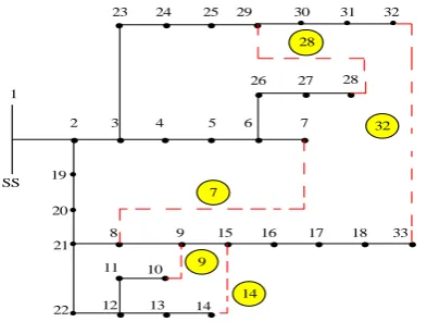
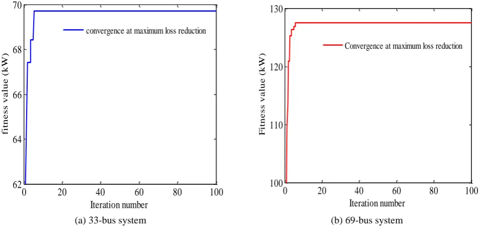
It is identified that the power loss is reduced and node voltage is improved when the switches 7, 9, 14, 28, 32are opened in test system-I whereas, the switches 69, 70, 14, 55, 61 are opened in test system-II. In this scenario, the corresponding optimal DNR is shown in Fig. 2 and 3 respectively that reveals the radial topology of the network. Furthermore, Fig. 4 shows the convergence characteristics of the mGWO algorithm; where the fitness value drastically dropped from a high value, and the mGWO can be attained optimal solution within the lesser iteration.
Fig. 2Optimal reconfiguration of 33-bus for minimum power loss by mGWO
Fig. 3Optimal reconfiguration of 69-bus for minimum power loss by mGWO
9 33 28 19 20 21 22
23 24 25
26 27 1
SS
15 16 17 18
2 3 4 5 6 7
8 9
10 11
12 13 14
14 7 28 32 31 32 30 29 38 69 70 14 55 61 1 SS 47 48 49 50
2 3 4 5 6 7 8 9 10 11 12 13
14
31
32 33 34 35
62
51 52
39 40 41 42
36 37 30 29 28 61 56 57 58 59 60 66 67 68 69
43 44 45 46 15 16 17 18 19 20 21 22 55 53 54
63 64 65
(a) 33-bus system (b) 69-bus system Fig. 4 Convergence characteristics of mGWO
5.3.2. Comparison of a viable solution
In an attempt to expose the predominance of mGWO algorithm in tackling DNR problem, the viable solution is obtained using CSA, IAICA, MBFOA, AWIDPSO, and RRA, and techniques including mGWO are contrasted in Tables 3 and 4 for test systems-I and II respectively. The improvement in power loss reduction of CSA, IAICA, MBFOA, AWIDPSO, and RRA, and mGWO from primary pattern is 63.84, 63.20, 68.19, 63.16, 69.72 and 68.95 kW respectively for test system-I. Similarly, CSA, IAICA, MBFOA, AWIDPSO, and mGWO are reduced the power loss from the initial configuration as 126.8685, 126.8658, 126.8765, 127.2395, and 127.4476 kW respectively for test system-II. Further, the algorithms’ potentiality of power loss reduction is illustrated in Fig. 5 for two test systems. It is experienced that the mGWO augmented the power loss diminishment massively in contrasted with the other competing methods in both test cases. Certainly, mGWO maximized the power loss reduction of 34.39 %, 56.53 % of test system-I and test system-II respectively. The mGWO method offered the least power losses, and similarly, regulated the node voltage by 5.85 %, 4.21 % of test system-I and test system-II respectively.
Fig. 5Comparisons of maximization of power loss reduction
Table 3Comparison of minimum power loss for 33 bus systems
Methods Optimal
Tie-switches
Power Loss (kW)
% of Power loss reduction
No. of Switches changed
% of Voltage regulation at Vmin Initial
condition 33, 34, 35, 36, 37 202.7100 --- --- 8.70
CSA 7, 9, 14, 32, 37 138.8700 31.49 4 6.63
IAICA 7, 9, 14, 32, 37 139.5100 31.18 4 6.75
MBFOA 7, 14, 28, 32, 36 134.5200 33.64 4 ---
AWIDPSO 7, 14, 11, 32, 28 133.7281 34.03 5 6.24
RRA 7, 14, 9, 32, 37 139.5500 31.16 4 6.63
mGWO 7, 9, 14, 28, 32 132.9939 34.39 5 5.85
0 20 40 60 80 100
62 64 66 68 70
Iteration number
fi
tn
e
s
s
v
a
lu
e
(
k
W)
convergence at maximum loss reduction
0 20 40 60 80 100
100 110 120 130
Iteration number
F
it
n
e
s
s
v
a
lu
e
(
k
W)
Convergence at maximum loss reduction
IAICA CS A MBFOA RRA AWIDPSO mGWO IAICA CS A MBFOA AWIDPSOmGWO
63.2kW 63.84kW
68.2kW
63.16kW
68.95kW
69.72kW
126.87kW 126.87kW
126.88kW
126.88kW
127.45kW
Table 4Comparison of minimum power loss for 69 bus systems
Methods Optimal
Tie-switches
Power Loss (kW)
% of Power loss reduction
No .of Switches changed
% of Voltage regulation at Vmin
Initial condition 69, 70, 71, 72, 73 225.4365 --- --- 9.17
CS 14, 57, 61 ,69, 70 98.5680 56.28 3 5.32
IAICA 14, 57, 61, 69, 70 98.5707 56.12 3 5.43
MBFOA 18, 43, 56, 61, 69 98.5600 56.28 4 ---
AWIDPSO 69, 18, 14, 57, 61 98.1970 56.44 4 5.02
mGWO 69, 70, 14, 55, 61 97.9889 56.53 3 4.21
5.3.3. Solution quality improvement
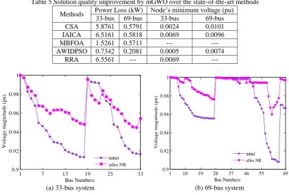
The performance of the mGWO algorithm while, performing stated objective is compared in Table 5 with well-known optimization techniques that are already proven their ability in solving the DNR problem. The power loss reduction rate is 5.8761, 6.5161, 1.5261, 0.7342 and 6.5561 kW greater than CSA, IAICA, MBFOA, AWIDPSO, and RRA respectively, of test system-I. Likewise, the power loss reduction rate is 0.5791, 0.5818, 0.5711, and 0.2081 kW greater than CSA, IAICA, MBFOA, and AWIDPSO respectively, of test system-II. The nodal pu minimum voltage obtained using mGWO is 0.0024, 0.0069, 0.0005 and 0.0069 higher than CSA, IAICA, AWIDPSO, and RRA respectively, of test system-I while in the case of test system-II the pu minimum nodal voltage is 0.010, 0.0096, and 0.0074 higher than CSA, IAICA, and AWIDPSO respectively. Fig. 6 shows the voltage profile of test systems-I and II, and the voltage profile is enhanced significantly after reconfiguration for the majority of the node.
Table 5 Solution quality improvement by mGWO over the state-of-the-art methods Methods Power Loss (kW) Node’s minimum voltage (pu)
33-bus 69-bus 33-bus 69-bus
CSA 5.8761 0.5791 0.0024 0.0101
IAICA 6.5161 0.5818 0.0069 0.0096
MBFOA 1.5261 0.5711 --- ---
AWIDPSO 0.7342 0.2081 0.0005 0.0074
RRA 6.5561 --- 0.0069 ---
(a) 33-bus system (b) 69-bus system
Fig. 6 Voltage profile improvement by mGWO
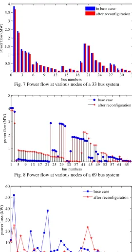
Power flow at a node and power loss in the branch are analyzed in Figs. 7 to 10 are for test systems I and II respectively to investigate the solution quality improvement while reconfiguring the distribution network. It observed that the power flow at all nodes in test system-I are reduced after reconfiguration. Conversely, the power flow at nodes 5-22, 41-45, 47, 48, 51-54, 57, 61 are increased. The investigation shows that the existing DS operates without overloading the feeder conductors after reconfiguration and also capable of supply extendable load. Consequently, power loss also streamlined among the branches. The power loss decreased some of the branches and is increased the remaining branches. Ultimately, the net power loss is reduced in the optimally restructured distribution network.
1 7 13 19 25 33
0.9 0.92 0.94 0.96 0.98 1
Bus Numbers
V
o
lt
a
g
e
m
a
g
n
it
u
d
e
(
p
u
)
initial after NR
1 10 19 28 37 46 55 69
0.9 0.92 0.94 0.96 0.98 1
Bus Numbers
V
o
lt
a
g
e
m
a
g
n
it
u
d
e
(
p
u
)
Fig. 7 Power flow at various nodes of a 33 bus system
Fig. 8 Power flow at various nodes of a 69 bus system
Fig. 9 Power loss at various branches of a 33 bus system
Fig. 10 Power loss at various branches of a 69 bus system
0 3 6 9 12 15 18 21 24 27 30 33
0.5 1 1.5 2 2.5 3 3.5 4
bus numbers
P
o
w
er
f
lo
w
(
M
W)
in base case after reconfiguration
1 5 9 13 17 21 25 29 33 37 41 45 49 53 57 61 65 69
1 2 3 4 5
bus numbers
p
o
w
e
r
fl
o
w
(
M
W)
base case
after reconfiguration
1 4 7 10 13 16 19 22 25 28 31 34 37
0 10 20 30 40 50 60
branch numbers
p
o
w
e
r
lo
ss
(
k
W)
base case
after reconfiguration
1 6 11 16 21 26 31 36 41 46 51 56 61 66 73
10 20 30 40 50
branch nombers
p
o
w
e
r
lo
ss
(
k
W)
5.3.4. Statistical comparison
Any evolutionary and swarm intelligence algorithm can provide an optimal solution for engineering problems. In this scenario, a standard analytical procedure has been employed to know whether it is a global optimum, or not. Therefore, the best solutions of the objective function that was obtained over 50 trials by IAICA, MBFOA, AWIDPSO, RRA, and mGWO algorithms for test system-I and Test system-II are statistically analyzed, and the best, average and the worst values among the final solutions are presented in Table 6 and Table 7 respectively. The mGWO algorithm found the best global fitness function and the average value of the fitness function smaller than the best value of other algorithms for both test systems.
Moreover, the RRA algorithm is exercised on test system-I only, and the final fitness function seems to strike at the premature solution as the best, average and worst values which are stayed same. Finally, the mGWO algorithm is ranked first while reconfiguring distribution system since it has the lowest standard deviation. During the procedure, it observed that 46 and 48 good quality fitness functions of test system-I, and test system-II out of 50 are relatively fallen between the best and average solution. The success rate is found to be 93.33 % and 86.67 % for test system-I and II, respectively while optimizing using the mGWO algorithm.
Table 6Statistical indices of the test results of a 33-bus system
Methods Power Loss (kW) Std
Dev. Rank Best Average Worst
Initial State 202.7060 --- --- -- ---
CSA 138.8700 --- --- --- ---
IAIC 139.5100 140.5700 142.3800 1.44 3 MBFOA 134.5200 150.5800 165.4000 15.44 4 AWIDPSO 133.7281 134.5154 135.8254 1.05 2 RRA 139.5500 139.5500 139.5500 0.00 --- mGWO 132.9939 133.6423 135.0000 1.00 1
Table 7Statistical indices of the test results of a 69-bus test system
Methods Power Loss (kW) Std
Dev. Rank Best Average Worst
Initial State 225.4365 --- --- --- ---
CSA 98.5680 --- --- --- ---
IAICA 98.5707 100.1577 103.8273 2.6283 3 MBFOA 98.5600 110.3033 155.58 28.51 4 AWIDPSO 98.1970 98.5885 100.0045 0.9038 2 mGWO 97.9889 98.1419 99.6200 0.8156 1
5.4. Case Study-II: Maximizing loss reduction in the presence of DG 5.4.1. Optimal location and size of DG
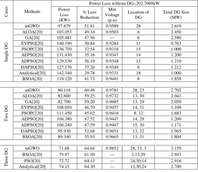
This case study is conducted under three circumstances. First, the system of the initial configuration is considered and standard load flow is employed to identify sensitive nodes; the most sensitive node is identified for DG placement, and the optimal size of DG is determined using the proposed algorithm for minimizing power loss. Second, the two most sensitive nodes are identified, and the optimal DG size is established using the proposed algorithm, again for maximizing the loss reduction. Conversely, in the third scenario, the three most sensitive nodes are preferred as the optimal locations and sizing of DG, which are determined using mGWO. Table 8 shows the optimal tie switch, DG sizes, and locations for all three circumstances.
Table 8 Feasible solutions obtained using mGWO for a 33-bus system
Particulars Without DG With DG
Single Two Three Power Loss (KW) 202.7069 97.6793 80.1161 71.68 % Loss Reduction --- 51.81 60.48 64.64 Min Voltage (p.u) 0.9131 0.9589 0.9781 0.9852
Location of DG --- 28 28, 23 28,23,3
DG’s Size (MW) --- 2.6190 1.232(28) 1.470(23)
0.858 (28) 1.033(23) 1.268(3)
5.4.2. Feasible solution
In Table 9, the feasible solution obtained using mGWO for the three circumstances at the maximum loss reduction is compared with those obtained using other methods. The proposed method achieves 51.81 % loss reduction from the initial state when integrating a single DG device, which is higher than that obtained using other methods; that is, 5.21%, 7.40%, 30.32%, 28.57 %, 25.68 %, 24.59 %, 23.19 %, 31.38 %, and 17.31 % for ALOA, GA, EVPSO, PSOPC, ADPSO, DAPSO, ANALYTICAL, and BSOA, respectively. Regarding the placement of two DG device, mGWO results in a loss reduction of 60.48 % from the fundamental configuration, which is superior to the values obtained using other algorithms: 3.01%, 3.12%, 25.85%, 28.11%, 24.69%, 24.59%, 16.48%, and 10.32% for ALOA, GA, EVPSO, PSOPC, AEPSO, ADPSO, DAPSO, and BSOA, respectively. For three DG devices, mGWO results in a loss reduction of 71.68% with regards to the initial configuration, higher than that obtained using other contestant algorithms: 10.37 %, 1.43%, and 3.33 % for BSOA, PSO, and ANALYTICAL, respectively.
Table 9 Comparison of feasible solutions obtained using various methods for the 33-bus system
Ca
se
s
Methods
Power Loss without DG=202.7069kW Power
Loss (KW)
% Loss Reduction
Min Voltage
(p.u)
Location of DG
Total DG Size (MW)
S
in
g
le DG
mGWO 97.679 51.81 0.9589 28 2.619
ALOA[20] 103.053 49.16 0.9503 6 2.450
GA[20] 105.481 47.96 --- 6 2.580
EVPSO[20] 140.190 30.84 0.9284 11 0.763
PSOPC[20] 136.750 32.54 0.9318 15 1.000
AEPSO[20] 131.430 35.16 0.9347 14 1.200
ADPSO[20] 129.530 36.10 0.9348 13 1.210
DAPSO[20] 127.170 37.26 0.9349 8 1.212
Analytical[20] 142.340 29.78 0.9331 18 1.000
BSOA[20] 118.120 41.73 0.9441 8 1.858
Two
DG
mGWO 80.116 60.48 0.9781 28, 23 2.702
ALOA[20] 82.600 59.25 0.9732 13, 30 2.041
GA[20] 82.700 59.20 0.9685 13, 29 2.050
EVPSO[20] 108.050 46.70 0.9457 14, 31 1.109
PSOPC[20] 111.450 45.02 0.9418 8, 12 1.683
AEPSO[20] 106.380 47.52 0.9447 14, 29 1.200
ADPSO[20] 106.240 47.59 0.9467 15, 30 1.171
DAPSO[20] 95.930 52.68 0.9651 13, 32 1.965
BSOA[20] 89.340 55.93 0.9665 13, 31 1.804
Th
re
e
DG
mGWO 71.68 64.64 0.9852 28, 23, 3 3.159
BSOA[20] 79.97 61.50 --- 3,13,29 2.943
PSO[20] 72.72 64.13 --- 24,30,14 2.916
Analytical[20] 74.15 64.30 --- 13,30,24 2.700
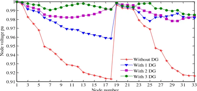
the existing DS. The effect of DG on voltage profile improvement is analyzed in Fig. 11, which compares the node voltage improvements without and with DG for all three scenarios. The voltage magnitude at all nodes is favorably altered.
Fig. 11 Power loss at various branches of a 33 bus system
6.
Conclusions
In this paper, a powerful metaheuristic algorithm, mGWO, is successfully employed to maximize power loss reduction in a DS through two methods. In the first method, the network reconfiguration is optimized, whereas in the second method, the penetration of DG in the existing DS and the selection of the required DG size are performed optimally, which results in voltage profile improvement. This is a complicated combinatorial, nondifferentiable, constrained optimization problem. In the first approach, the difference in a power loss of all branch sections of the feeder, as well as the network reconfiguration is deemed an objective function. In the second approach, the difference between the power loss that occurs in the system without and with DG is considered the objective function. To identify a weak node, the loss sensitivity factor approach is incorporated in the forward/backward-sweep distribution load flow algorithm.
The mGWO algorithm is used to solve this problem; this algorithm emulates the inherent behavior of gray wolves, which encircle, hunt, and attack their prey. The strategic ratio between the global and local searches of the algorithm varies linearly from a high value to zero in the basic GWO. This may decrease the diversity of global optima. When obtaining the best fitness value from local optima, the strategic balance between global and local search is varied exponentially from a high value to zero in the mGWO method. Simulation is performed on 33- and 69-bus DSs for network reconfiguration and a 33-bus system for DG implementation. The simulation results are compared with those of previous studies; the optimal determination of a tie switch is unique, and the acquired configuration is autonomous of the initial state of the DS. Moreover, this paper provides a solution to reduce massive power loss in radial DSs, and the improvement brought about by this solution is analyzed in detail. Hence, the proposed mGWO is a robust and viable algorithm for discovering the global optimum DS reconfiguration, and ultimately, the numerical outcomes are helpful for power distribution companies wishing to inject real power into a DS through PV-type DG. The penetration of a different type of DG, placement of DG after reconfiguration, and performing network reconfiguration in the presence of DG are topics for future research.
Conflicts of Interest
The authors declare no conflict of interest.
Acknowledgement
The authors would like to thank Misrimal Navajee Munoth Jain Engineering College, Chennai, India for providing infrastructural facilities to conduct the research work.
1 3 5 7 9 11 13 15 17 19 21 23 25 27 29 31 33
0.91 0.92 0.93 0.94 0.95 0.96 0.97 0.98 0.99 1
Node number
N
o
d
e
v
o
lt
ag
e
p
u
Nomenclature
k
I kth branch current t Current iteration
max
k
I kth branch maximum current A, C Coefficient vectors
,
k k
R X Resistance and reactance of the line section
between buses p and q a Acceleration vector
k
P, Qk Real and reactive power is flowing out of
bus p r1 Random vectors in [0 1]
q
P, Qq Real and reactive power is flowing out of
bus q T Maximum iteration
,
q L
P , Qq L, Real and reactive power load at bus q NL Number of fundamental loops
p p
V Voltage magnitude and the angle at bus p Lj jth loop vector
q q
V Voltage magnitude and the angle at bus q SWj d, dth branch or closed switch in the jth loop
,
k loss
P Real power loss in the branch segment k NP Population size
, , ,
q eff q eff
P Q Effective active and reactive power
supplied beyond the bus q LSW
Total number of the closed switch in the jth loop at loop vector matrix
ss
N Number of substations 1.. 3
i NP
g g
P P Size of distributed generation
' ' , , ,
q eff q eff
P Q
Effective active and reactive power supplied beyond the bus q after reconfiguration
ij
Pseudorandom integer values are drawn from the discrete uniform distribution between any two intervals.
, ,?
bus br
DG
N N
N
Number of bus, branch and distributed generation
List of abbreviations
CSA Cuckoo search algorithm
g
P , Qg Real and reactive power supplied by DG GA Genetic Algorithm D Distance from source to the DG location in
km
PSO Particle Swarm Optimization RRA Runner-root algorithm
L The total length of the feeder from source
to bus k in km EVPSO Escape Velocity PSO
Loss P
Net power loss after reconfiguration PSOPC PSO with Passive Congregation
DG Loss
P
Net power loss after DG placed AEPSO PSO with Area Extension
D Position vector of each hunter from any other hunters ADPSO Adaptive Dissipative PSO
prey
X Position vector of the prey DAPSO Dynamic Adaptation of PSO
wolf
X Position vector of the gray wolf BSOA Backtracking search optimization algorithm
Appendix
Algorithm parameter Population size (NP) : 30 Maximum number of iteration : 100
System voltage limits V-Min : 0.95pu
V-Max : 1.05pu
References
[1] M. E. Baran and F. F. Wu, “Network reconfiguration in distribution systems for loss reduction and load balancing,” IEEE Power Engineering Review, vol. 9, pp. 101-102, April 1989.
[2] H. D. Chiang and R. Jean-Jumeau, “Optimal network reconfigurations in distribution systems. II. Solution algorithms and numerical results,” IEEE Transactions on Power Delivery, vol. 5, pp. 1568-1574, July 1990.
[3] B. Venkatesh, R. Rakesh, and H. B. Gooi, “Optimal reconfiguration of radial distribution systems to maximize loadability,” IEEE Transactions on Power Systems, vol. 19, pp.260-266, February 2004.
[5] C. T. Su, C. F. Chang, and J. P. Chiou, “Distribution network reconfiguration for loss reduction by ant colony search algorithm,” Electric Power Systems Research, vol. 75, pp. 190-199, August 2005.
[6] F. Rivas-Davalos and M. Irving, “The edge-set encoding in evolutionary algorithms for power distribution network planning problem part I: Single-objective optimization planning,” Proc. IEEE Con. Electronics, Robotics and Automotive Mechanics Conference, September 2006.
[7] C. Wang and H. Z. Cheng, “Optimization of network configuration in large distribution systems using plant growth simulation algorithm,” IEEE Transactions on Power Systems, vol. 23, pp. 119-126, February 2008.
[8] K. Sathish Kumar and T. Jayabarathi, “Power system reconfiguration and loss minimization for a distribution systems using bacterial foraging optimization algorithm,” International Journal of Electrical Power & Energy Systems, vol. 36, pp. 13-17, March 2012.
[9] T. T. Nguyen and A. V. Truong, “Distribution network reconfiguration for power loss minimization and voltage profile improvement using cuckoo search algorithm,” International Journal of Electrical Power & Energy Systems, vol. 68, pp. 233-242, June 2015.
[10] A. Swarnkar, N. Gupta, and K. R. Niazi, “Adapted ant colony optimization for efficient reconfiguration of balanced and unbalanced distribution systems for loss minimization,” Swarm and Evolutionary Computation, vol. 1, pp. 129-137, September 2011.
[11] S. H. Mirhoseini, S. M. Hosseini, M. Ghanbari, and M. Ahmadi, “A new improved adaptive imperialist competitive algorithm to solve the reconfiguration problem of distribution systems for loss reduction and voltage profile improvement,” International Journal of Electrical Power & Energy Systems, vol. 55, pp. 128-143, February 2014.
[12] S. Naveen, K. Sathish Kumar, and K. Rajalakshmi, “Distribution system reconfiguration for loss minimization using modified bacterial foraging optimization algorithm,” International Journal of Electrical Power & Energy Systems, vol. 69, pp. 90-97, July 2015.
[13] M. Subramaniyan, S. Subramaniyan, V. Jawalkar, and M. Veerasamy, “Adaptive weighted improved discrete particle swarm optimization for optimal distribution network reconfiguration,” Journal of Computational and Theoretical Nanoscience, vol. 14, pp. 3344-3350, July 2017.
[14] C. T. Su and C. S. Lee, “Network reconfiguration of distribution systems using improved mixed-integer hybrid differential evolution,” IEEE Transactions on Power Delivery, vol. 18, pp. 1022-1027, July 2003.
[15] T. Niknam, “An efficient hybrid evolutionary algorithm based on PSO and ACO for distribution feeder reconfiguration,” European Transactions on Electrical Power, vol. 20, pp. 575-590, July 2010.
[16] T. T. Nguyen, A. V. Truong, Q. T. Nguyen, and T. A. Phung, “Multiobjective electric distribution network reconfiguration solution using runner-root algorithm,” Applied Soft Computing, vol. 52, pp. 93-108, March 2017.
[17] S. Manikandan, S. Sasidharan, J. Viswanatharao, and V. Moorthy, “Fuzzy satisfied multiobjective distribution network reconfiguration: an application of adaptive weighted improved discrete particle swarm optimization,” International Review on Modelling and Simulations, vol. 10, pp. 247-257, August 2017.
[18] A. Y. Abdelaziz, E. S. Ali, and S. M. Abd Elazim, “Flower pollination algorithm and loss sensitivity factors for optimal sizing and placement of capacitors in radial distribution systems,” International Journal of Electrical Power & Energy Systems, vol. 78, pp. 207-214, June 2016.
[19] E. S. Ali, S. M. Abd Elazim, and A. Y. Abdelaziz, “Improved harmony algorithm and power loss index for optimal locations and sizing of capacitors in radial distribution systems,” International Journal of Electrical Power & Energy Systems, vol. 80, pp. 252-263, September 2016.
[20] E. S. Ali, S. M. Abd Elazim, and A. Y. Abdelaziz, “Ant lion optimization algorithm for renewable distributed generations,” Energy, vol. 116, pp. 445-458, December 2016.
[21] S. Mirjalili, S. M. Mirjalili, and A. Lewis, “Grey wolf optimizer,” Advances in Engineering Software, vol. 69, pp. 46-61, March 2014.
[22] J. Rameshkumar, S. Ganesan, S. Subramanian, and M. Abirami, “Cost, emission and reserve pondered pre-dispatch of thermal power generating units coordinated with real coded grey wolf optimisation,” IET Generation, Transmission & Distribution, vol. 10, pp. 972-985, March 2016.
[23] N. Mittal, U. Singh, and B. S. Sohi, “Modified grey wolf optimizer for global engineering optimization,” Applied Computational Intelligence and Soft Computing, vol. 2016, pp. 1-16, 2016.
Copyright© by the authors. Licensee TAETI, Taiwan. This article is an open access article distributed under the terms and conditions of the Creative Commons Attribution (CC BY-NC) license