When Are Overcomplete Topic Models Identifiable? Uniqueness of Tensor Tucker Decompositions with Structured Sparsity

(1)

When Are Overcomplete Topic Models Identifiable?

Uniqueness of Tensor Tucker Decompositions

with Structured Sparsity

Animashree Anandkumar [email protected]

Department of Electrical Engineering and Computer Science University of California, Irvine

Engineering Hall, #4408 Irvine, CA 92697, USA

Daniel Hsu [email protected]

Department of Computer Science Columbia University

1214 Amsterdam Avenue, #0401 New York, NY 10027, USA

Majid Janzamin [email protected]

Department of Electrical Engineering and Computer Science University of California, Irvine

Engineering Hall, #4407 Irvine, CA 92697, USA

Sham Kakade [email protected]

Department of Computer Science Department of Statistics

University of Washington Seattle, WA 98195, USA

Editor:Benjamin Recht

Abstract

(2)

Anandkumar, Hsu, Janzamin and Kakade

Keywords: overcomplete representations, topic models, generic identifiability, tensor decomposition

1. Introduction

The performance of many machine learning methods is hugely dependent on the choice of data representations or features. Overcomplete representations, where the number of features can be greater than the dimensionality of the input data, have been extensively employed, and are arguably critical in a number of applications such as speech and computer vision (Bengio et al., 2012). Overcomplete representations are known to be more robust to noise, and can provide greater flexibility in modeling (Lewicki et al., 1998). Unsupervised estimation of overcomplete representations has been hugely popular due to the availability of large-scale unlabeled samples in many applications.

A probabilistic framework for incorporating features posits latent or hidden variables that can provide a good explanation to the observed data. Overcomplete probabilistic models can incorporate a much larger number of latent variables compared to the observed dimensionality. In this paper, we characterize the conditions under which overcomplete latent variable models can be identified from their observed moments.

For any parametric statistical model, identifiability is a fundamental question of whether the model parameters can be uniquely recovered given the observed statistics. Identifiability is crucial in a number of applications where the latent variables are the quantities of in-terest, e.g. inferring diseases (latent variables) through symptoms (observations), inferring communities (latent variables) via the interactions among the actors in a social network (observations), and so on. Moreover, identifiability can be relevant even in predictive set-tings, where feature learning is employed for some higher level task such as classification. For instance, non-identifiability can lead to the presence of non-isolated local optima for optimization-based learning methods, and this can affect their convergence properties, e.g., see Uschmajew (2012).

In this paper, we characterize identifiability for a popular class of latent variable models, known as the admixture or topic models (Blei et al., 2003; Pritchard et al., 2000). These are hierarchical mixture models, which incorporate the presence of multiple latent states (i.e. topics) in each document consisting of a tuple of observed variables (i.e. words). Pre-vious works have established that the model parameters can be estimated efficiently using low order observed moments (second and third order) under some non-degeneracy assump-tions, e.g. Anandkumar et al. (2012b); Anandkumar et al. (2012); Arora et al. (2012b). However, these non-degeneracy conditions imply that the model is undercomplete, i.e., the latent dimensionality (number of topics) cannot exceed the observed dimensionality (word vocabulary size). In this paper, we remove this restriction and consider overcomplete topic models, where the number of topics can far exceed the word vocabulary size.

(3)

h

y1 y2 y2r

x1 xn xn+1 x2n x(2r−1)n+1 x2rn A A A

A A A

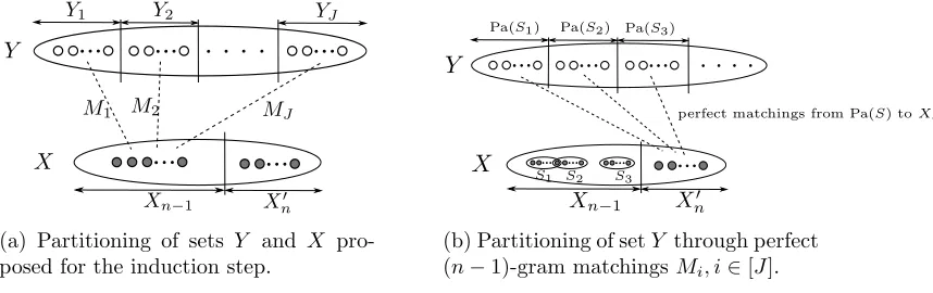
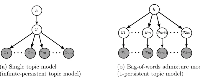
Figure 1: Hierarchical structure of the n-persistent topic model is illustrated for 2rnnumber of words (views) wherer≥1 is an integer. A single topicyj, j∈[2r], is chosen for each sequence ofn

views{x(j−1)n+1, . . . , x(j−1)n+n}. MatrixAis the population structure or topic-word matrix.

and speech, and can lead to a more faithful representation. In addition, we establish that the presence of topic persistence is central towards obtaining model identifiability in the overcomplete regime, and we provide an in-depth analysis of this phenomenon in this paper.

1.1 Summary of Results

In this paper, we provide conditions forgeneric1 _{model identifiability of overcomplete topic} models given observable moments of a certain order (i.e., having a certain number of words in each document). We introduce the notion of topic persistence, and analyze its effect on identifiability. We establish identifiability in the presence of a novel combinatorial object, referred to asperfectn-gram matching, in the bipartite graph from topics to words. Finally, we prove that random structured topic models satisfy these criteria, and are thus identifiable in the overcomplete regime.

1.1.1 Persistent Topic Model

We first introduce the n-persistent topic model, where the parameter n determines the persistence level of a common topic in a sequence of n successive words. For instance, in Figure 1, the sequence of successive wordsx1, . . . , xnshare a common topicy1, and similarly, the words xn+1, . . . , x2n share topic y2, and so on. The n-persistent model reduces to the popular “bag-of-words” model, whenn= 1, and to the single topic model (i.e. only one topic in each document) when n→ ∞. Intuitively, topic persistence aids identifiability since we have multipleviewsof the common hidden topic generating a sequence of successive words. We establish that the bag-of-words model (with n = 1) is too non-informative about the topics in the overcomplete regime, and is therefore, not identifiable. On the other hand,n -persistent overcomplete topic models with n_≥2 can become identifiable, and we establish a set of transparent conditions for identifiability.

1.1.2 Deterministic Conditions for Identifiability

Our sufficient conditions for identifiability are in the form of expansion conditions from the latent topic space to the observed word space. In the overcomplete regime, there are more topics than words in the vocabulary, and thus it is impossible to have expansion on the bipartite graph from topics to words, i.e., the graph encoding the sparsity pattern of

1. A model is generically identifiable, if all the parameters in the parameter space are identifiable, almost surely. Refer to Definition 2 for more discussion.

3

Figure 1: Hierarchical structure of the n-persistent topic model is illustrated for 2rn number of words (views) wherer _≥1 is an integer. A single topic yj, j ∈ [2r], is chosen for each

sequence ofnviews_{x(j−1)n+1, . . . , x(j−1)n+n}. MatrixAis the population structure or

topic-word matrix.

and speech, and can lead to a more faithful representation. In addition, we establish that the presence of topic persistence is central towards obtaining model identifiability in the overcomplete regime, and we provide an in-depth analysis of this phenomenon in this paper.

1.1 Summary of Results

In this paper, we provide conditions forgeneric1 _{model identifiability of overcomplete topic}

models given observable moments of a certain order (i.e., having a certain number of words in each document). We introduce the notion oftopic persistence, and analyze its effect on identifiability. We establish identifiability in the presence of a novel combinatorial object, referred to asperfectn-gram matching, in the bipartite graph from topics to words. Finally, we prove that random structured topic models satisfy these criteria, and are thus identifiable in the overcomplete regime.

1.1.1 Persistent Topic Model

We first introduce the n-persistent topic model, where the parameter n determines the persistence level of a common topic in a sequence of n successive words. For instance, in Figure 1, the sequence of successive wordsx1, . . . , xnshare a common topicy1, and similarly,

the words xn+1, . . . , x2n share topic y2, and so on. The n-persistent model reduces to the

popular “bag-of-words” model, whenn= 1, and to the single topic model (i.e. only one topic in each document) whenn→ ∞. Intuitively, topic persistence aids identifiability since we have multipleviewsof the common hidden topic generating a sequence of successive words. We establish that the bag-of-words model (with n = 1) is too non-informative about the topics in the overcomplete regime, and is therefore, not identifiable. On the other hand, n -persistent overcomplete topic models with n_≥2 can become identifiable, and we establish a set of transparent conditions for identifiability.

(4)

1.1.2 Deterministic Conditions for Identifiability

Our sufficient conditions for identifiability are in the form of expansion conditions from the latent topic space to the observed word space. In the overcomplete regime, there are more topics than words in the vocabulary, and thus it is impossible to have expansion on the bipartite graph from topics to words, i.e., the graph encoding the sparsity pattern of the topic-word matrix. Instead, we impose an expansion constraint from topics to “higher order” words, which allows us to incorporate overcomplete models. We establish that this condition translates to the presence of a novel combinatorial object, referred to as the

perfect n-gram matching, on the topic-word bipartite graph. Intuitively, the perfectn-gram matching condition implies “diversity” among the higher-order word supports for different topics which leads to identifiability. In addition, we present trade-offs among the following quantities: number of topics, size of the word vocabulary, the topic persistence level, the order of the observed moments at hand, the minimum and maximum degrees of any topic in the topic-word bipartite graph, and the Kruskal rank (Kruskal, 1976) of the topic-word matrix, under which identifiability holds. To the best of our knowledge, this is the first work to provide conditions for characterizing identifiability of overcomplete topic models with structured sparsity.

As a corollary of our result, we also show that the expansion condition can be removed if the topic-word matrix is full column rank (and therefore undercomplete) and the model is persistent with persistence level at least two.

1.1.3 Identifiability of Random Structured Topic Models

We explicitly characterize the regime of identifiability for the random setting, where each topiciis supported on a random set ofdiwords. Therefore, the bipartite graph from topics

to words is a random graph with prescribed degrees for topics. For this random model with q topics,p-dimensional word vocabulary, and topic persistence leveln, whenq=O(pn_{) and}

Θ(logp) ≤ di ≤ Θ(p1/n), for all topics i, the topic-word matrix is identifiable from 2nth

order observed moments with high probability. Intuitively, the upper bound on the degrees diis needed to limit the overlap of word supports among different topics in the overcomplete

regime: as the number of topics q increases (i.e., n increases in the above degree bound), the degree needs to be correspondingly smaller to ensure identifiability, and we make this dependence explicit. Intuitively, as the extent of overcompleteness increases, we need sparser connections from topics to words to ensure sufficient diversity in the word supports among different topics. The lower bound on the degrees is required so that there are enough edges in the topic-word bipartite graph so that various topics can be distinguished from one another. Furthermore, we establish that the size condition q =O(pn) for identifiability is tight.

As in the deterministic case, we also argue the result in the undercomplete setting and show that ifq_≤O(p) anddi≥Ω(logp), then the topic-word matrix is identifiable from 2nth

(5)

1.1.4 Implications on Uniqueness of Overcomplete Tucker and CP Tensor Decompositions

We establish that identifiability of an overcomplete topic model is equivalent to uniqueness of decomposition of the observed moment tensor (of a certain order). Our identifiability results for persistent topic models imply uniqueness of a structured class of tensor decompositions, which is contained in the class of Tucker decompositions, but is more general than the

candecomp/parafac(CP) decomposition (Kolda and Bader, 2009). This sub-class of Tucker decompositions involves structured sparsity and symmetry constraints on the core tensor, and sparsity constraints on theinverse factorsof the Tucker decomposition. The structural constraints on the Tucker tensor decomposition are related to the topic model as follows: the sparsity and symmetry constraints on the core tensor are related to the persistence property of the topic model, and the sparsity constraints on the inverse factors are equivalent to the sparsity constraints on the topic-word matrix. Forn-persistent topic model withn= 1 (bag-of-words model), the tensor decomposition is a general Tucker decomposition, where the core tensor is fully dense, while forn_{→ ∞} (single-topic model), the tensor decomposition reduces to a CP decomposition, i.e. the core tensor is a diagonal tensor. For a finite persistence leveln, in between these two extremes, the core tensor satisfies certain sparsity and symmetry constraints, which becomes crucial towards establishing identifiability in the overcomplete regime.

1.2 Overview of Techniques

We now provide a short overview of the techniques employed in this paper.

Recap of Identifiability Conditions in Under-complete Setting (Expansion Conditions on Topic-Word Matrix): Our approach is based on the recent results of Anandkumar et al. (2012), where conditions for identifiability of topic models are derived, given pairwise ob-served moments (specifically, co-occurrence of word-pairs in documents). Consider a topic model with q topics and observed word vocabulary of size p. Let A ∈ Rp×q _{denote the}

topic-word matrix. Expansion conditions are imposed in Anandkumar et al. (2012) on the topic-word bipartite graph which imply that (generically) the sparsest vectors in the column span ofA, denoted by Col(A), are the columns of Athemselves. Thus the topic-word ma-trix A is identifiable from pairwise moments under expansion constraints. However, these expansion conditions constrain the model to be under-complete, i.e., the number of topics q ≤p, the size of the word vocabulary. Therefore, the techniques derived in Anandkumar et al. (2012) are not directly applicable here since we consider overcomplete models.

Identifiability in Overcomplete Setting and Why Topic-Persistence Helps: Pairwise mo-ments are thus not sufficient for identifiability of overcomplete models, and the question is whether higher order moments can yield identifiability. We can view the higher order moments as pairwise moments of another equivalent topic model, which enables us to apply the techniques of Anandkumar et al. (2012). The key question is whether we have expansion in the equivalent topic model, which implies identifiability. For a general topic model (with-out any topic persistence constraints), it can be shown that for identifiability, we require expansion of thenth_-order_{Kronecker product} _{of the original topic-word matrix} _A_{, denoted} by A⊗n ∈ Rpn_×_qn

(6)

models are not identifiable in general. On the other hand, we show that imposing the con-straint of topic persistence can lead to identifiability. For an-persistent topic model, given (2n)th_{-order moments, we establish that identifiability occurs when the}_nth_-order_Khatri-Rao

productofA, denoted by An_∈_Rpn_×_q

, expands. Note that the Khatri-Rao productAn_is

a sub-matrix of the Kronecker productA⊗n, and the Khatri-Rao product An can expand as long as q _≤ pn. Thus, the property of topic persistence is central towards achieving identifiability in the overcomplete regime.

First-Order Approach for Identifiability of Overcomplete Models (Expansion of n-gram Topic-Word Matrix): We refer to An _∈ _Rpn_×_q

as the n-gram topic-word matrix, and intuitively, it relates topics to n-tuple words. Imposing the expansion conditions derived in Anandkumar et al. (2012) on An _{implies that (generically) the sparsest vectors in}

Col(An_{), are the columns of}_An_{themselves. Thus, the topic-word matrix}_A_{is identifiable}

from (2n)th_{-order moments for a} _n_{-persistent topic model. We refer to this as the} “first-order” approach since we directly impose the expansion conditions of Anandkumar et al. (2012) on An_{, without exploiting the additional structure present in} _An_.

Why the First-Order Approach is not Enough: Note that An _∈ _Rpn_×_q

matrix relates topics to n-tuples of words. Thus, the entries of An are highly correlated, even if the original topic-word matrixAis assumed to be randomly generated. It is non-trivial to derive conditions on A, so that An _{expands. Moreover, we establish that} _An _{fails to expand}

on “small” sets, as required in Anandkumar et al. (2012), when the degrees are sufficiently different2. Thus, the first-order approach is highly restrictive in the overcomplete setting.

Incorporating Rank Criterion: Note that An is highly structured: the columns ofAn matrix possess a tensor3rank of 1, whenn >1. This can be incorporated in our identifiabil-ity criteria as follows: we provide conditions under which the sparsest vectors in Col(An_),

which also possess a tensor rank of 1, are the columns of An themselves. This implies identifiability of a n-persistent topic model, when given access to (2n)th_{-order moments.} Note that when a small number of columns ofAn _{are combined, the resulting vector}

can-not possess a tensor rank of 1, and thus, we can rule out that such sparse combinations of columns using the rank criterion. The maximum such number is at least theKruskal rank4

ofA. Thus, sparse combinations of columns of A(up to the Kruskal rank) can be ruled out using the rank criterion, and we require expansion on An only on large sets of topics (of size larger than the Kruskal rank). This agrees with the intuition that when the topic-word matrixAhas a larger Kruskal rank, it should be easier to identifyA, since the Kruskal rank is related to themutual incoherence5 _{among the columns of} _A_{, see Gandy et al. (2011).}

2. ForAnto expand on a set of sizes≥2, it is necessary thats· dmin+n−1 n

≥s+ dmax+n−1 n

, wheredmin

anddmax are the minimum and maximum degrees, andnis the extent of overcompleteness: q= Θ(pn).

When the model is highly overcomplete (large n) and we require small set expansion (small s), the degrees need to be nearly the same. Thus, it is desirable to impose expansion only on large sets, since it allows for more degree diversity.

3. When any column ofAn_∈_Rpn×q _{(of length}_pn_{) is reshaped as a}_nth_{-order tensor}_T _∈_Rp×p×···×p_{, the} tensorT is rank 1.

4. The Kruskal rank is the maximum number k such that every k-subset of columns of A are linearly independent. Note that the Kruskal rank is equal to the rank of A, whenAhas full column rank. But this cannot happen in the overcomplete setting.

(7)

Notion of Perfect n-gram Matching and Final Identifiability Conditions: Thus, we es-tablish identifiability of overcomplete topic models subject to expansion conditionsAn on sets of size larger than the Kruskal rank of the topic-word matrix A. However, it is desir-able to impose transparent and interpretdesir-able conditions directly onAfor identifiability. We introduce the notion ofperfect n-gram matching on the topic-word bipartite graph, which ensures that each topic can be uniquely matched to a n-tuple word. This combined with a lower bound on the Kruskal rank provides the final set of deterministic conditions for identifiability of the overcomplete topic model. Intuitively, we require that the columns of A be sparse, while still maintaining a large enough Kruskal rank; in other words, the topics have to be sparse and have sufficiently diverse word supports. Thus, we establish identifiability under a set of transparent conditions on the topic-word matrix A, consisting of perfectn-gram matching condition and a lower bound on the Kruskal rank ofA.

Analysis under Random-Structured Topic-Word Matrices: Finally, we establish that the derived deterministic conditions are satisfied when the topic-word bipartite graph is ran-domly generated, as long as the degrees satisfy certain lower and upper bounds. Intuitively, a lower bound on the degrees of the topics is required to have degree concentration on various subsets so that expansion can occur, while the upper bound is required so that the Kruskal rank of the topic-word matrix is large enough compared to the sparsity level. Here, the main technical result is establishing the presence of a perfect n-gram matching in a random bipartite graph with a wide range of degrees. We present a greedy and a recursive mechanism for constructing such a n-gram matching for overcomplete models, which can be relevant even in other settings. For instance, our results imply the presence of a perfect matching when the edges of a bipartite graph are correlated in a structured manner, as given by the Khatri-Rao product.

1.3 Related Works

We now summarize some recent related works in the area of identifiability and learning of latent variable models.

1.3.1 Identifiability, Learning and Applications of Overcomplete Latent Representations

(8)

of the model, and here, the dimensionality of the latent space is required to be of the same order as the observed space dimensionality. In contrast, a number of recent works analyze

generic identifiability of overcomplete CP decomposition, which is weaker than strict iden-tifiability, e.g. Jiang and Sidiropoulos (2004); Lathauwer (2006); Stegeman et al. (June 2006); De Lathauwer et al. (2007); Chiantini and Ottaviani (2012); Bocci et al. (2013); Chiantini et al. (2013). These works assume that the factors (i.e. the components) of the CP decomposition are generically drawn and provide conditions for uniqueness. They allow for the latent dimensionality to be much larger (polynomially larger) than the observed dimensionality. These results on the uniqueness of CP decompositions also lead to identifi-ability of other latent variable models, such as latent tree models, e.g. Allman et al. (2009, Dec. 2012), and the single-topic model, or more generally latent Dirichlet allocation (LDA). Recently, Goyal et al. (2013) proposed an alternative framework for overcomplete ICA mod-els based on the eigen-decomposition of the reweighted covariance matrix (or higher order moments), where the weights are the Fourier coefficients. However, their approach requires independence of sources (i.e. latent topics in our context), which is not imposed here.

In contrast to the above works dealing with the CP tensor decomposition, we require uniqueness for a more general class of tensor decompositions, in order to establish identifia-bility of topic models with arbitrarily correlated topics. We establish that our class of tensor decomposition is contained in the class ofTuckerdecompositions which is more general than CP decomposition. Moreover, we explicitly characterize the effect of the sparsity pattern of the factors (i.e., the topic-word matrix) on model identifiability, while all the previous works based on generic identifiability assume fully dense factors (since sparse factors are not generic). For a general overview of tensor decompositions, see Kolda and Bader (2009); Landsberg (2012).

1.3.2 Identifiability and Learning of Undercomplete/Over-determined latent Representations

Much of the theoretical results on identifiability and learning of the latent variable models are limited to non-singular models, which implies that the latent space dimensionality is at most the observed dimensionality. We outline some of the recent works below.

(9)

of higher computational complexity for overcomplete CP tensor decomposition. However, it is not clear how the sparsity constraints affect the guarantees of such methods. Moreover, these approaches cannot handle general topic models, where the distribution of the topic proportions is not limited to these classes (i.e. either single topic or Dirichlet distribution), and we require tensor decompositions which are more general than the CP decomposition. There are many other works which consider learning mixture models when multiple views are available. See Anandkumar et al. (2012) for a detailed description of these works. Recently, Rabani et al. (2012) consider learning discrete mixtures given a large number of “views”, and they refer to the number of views as the sampling aperture. They establish improved recovery results (in terms of `1 bounds) when sufficient number of views are

available (2k−1 views for a k-component mixture). However, their results are limited to discrete mixtures or single-topic models, while our setting can handle more general topic models. Moreover, our approach is different since we incorporate sparsity constraints in the topic-word distribution. Another series of recent works by Arora et al. (2012a,b) employ approaches based on non-negative matrix factorization (NMF) to recover the topic-word matrix. These works allow models with arbitrarily correlated topics, as considered here. They establish guaranteed learning when every topic has ananchor word, i.e. the word is uniquely generated from that topic, and does not occur under any other topic. Note that the anchor-word assumption cannot be satisfied in the overcomplete setting.

Our work is closely related to the work of Anandkumar et al. (2012) which considers identifiability and learning of topic models under expansion conditions on the topic-word matrix. The work of Spielman et al. (2012b) considers the problem of dictionary learning, which is closely related to the setting of Anandkumar et al. (2012), but in addition assumes that the coefficient matrix is random. However, these works in Anandkumar et al. (2012); Spielman et al. (2012b) can handle only the under-complete setting, where the number of topics is less than the dimensionality of the word vocabulary (or the number of dictionary atoms is less than the number of observations in Spielman et al. (2012b)). We extend these results to the overcomplete setting by proposing novel higher order expansion conditions on the topic-word matrix, and also incorporate additional rank constraints present in higher order moments.

1.3.3 Dictionary Learning/Sparse Coding

(10)

predic-Anandkumar, Hsu, Janzamin and Kakade

tive tasks here, but the task of recovering the underlying latent representation. Hillar and Sommer (2011) consider the problem of identifiability of sparse coding and establish that when the dictionary succeeds in reconstructing a certain set of sparse vectors, then there exists a unique sparse coding, up to permutation and scaling. However, our setting here is different, since we do not assume that a sparse set of topics occur in each document.

2. Model

We first introduce some notations, and then we provide the persistent topic model.

2.1 Notation

The set _{1,2, . . . , n_} is denoted by [n] := _{1,2, . . . , n_}. Given a set X = _{1, . . . , p_}, set X(n) denotes all orderedn-tuples generated fromX. The cardinality of a setS is denoted by |S|. For any vector u (or matrix U), the support is denoted by Supp(u), and the `0

norm is denoted by _ku_k0, which corresponds to the number of non-zero entries of u, i.e.,

kuk0:=|Supp(u)|. For a vectoru∈Rq, Diag(u)∈Rq×qis the diagonal matrix with vector

u on its diagonal. The column space of a matrix A is denoted by Col(A). Vector ei ∈Rq

is the i-th basis vector, with the i-th entry equal to 1 and all the others equal to zero. For A_∈_Rp×q _and_B _∈_Rm×n_{, the}_Kronecker_product_A_⊗_B _∈_Rpm×qn_{is defined as (Golub and}

Loan, 2012)

A_⊗B =     

a11B a12B · · · a1qB a21B a22B · · · a2qB

..

. ... . .. ... ap1B ap2B · · · apqB

    ,

and forA = [a1|a2| · · · |ar]∈Rp×r and B = [b1|b2| · · · |br]∈Rm×r, the Khatri-Rao product AB _∈_Rpm×r _{is defined as}

AB = [a1⊗b1|a2⊗b2| · · · |ar⊗br]. 2.2 Persistent Topic Model

In this section, the n-persistent topic model is introduced and this imposes an additional constraint, known as topic persistence on the popular admixture model(Blei et al., 2003; Pritchard et al., 2000; Nguyen, 2012). The n-persistent topic model reduces to the bag-of-words admixture model whenn= 1.

An admixture model specifies a q-dimensional vector of topic proportionsh∈∆q−1 := {u _∈ Rq : ui ≥ 0,Piq=1ui = 1} which generates the observed variables xl ∈ Rp through

vectors a1, . . . , aq ∈ Rp. This collection of vectors ai, i ∈ [q], is referred to as the popula-tion structure or the topic-word matrix(Nguyen, 2012). For instance,ai is the conditional

distribution of words given topic i. The latent variable h is a q dimensional random vec-tor h := [h1, . . . , hq]> known as proportion vector. A prior distribution P(h) over the

(11)

The n-persistent topic model has a three-level multi-view hierarchy in Figure 1. 2rn number of words (views) are shown in the model for some integerr ≥1. In this model, a common hidden topic is persistent for a sequence ofnwords _{x₍_j₋₁₎_n₊₁, . . . , x₍_j₋₁₎_n₊_n_}, j_∈ [2r]. Note that the random observed variables (words) are exchangeable within groups of sizen, wherenis the persistence level, but are not globally exchangeable.

We now describe a linear representation of the n-persistent topic model, on lines of Anandkumar et al. (2012b), but with extensions to incorporate persistence. Each random variable yj, j ∈ [2r], is a discrete valued random variable taking one of the q possibilities

{1, . . . , q_}, i.e., yj ∈ [q] for j ∈ [2r]. In the n-persistent model, a single common topic

is chosen for a sequence of n words _{x₍_j₋₁₎_n₊₁, . . . , x₍_j₋₁₎_n₊_n_}, j _∈ [2r], i.e., the topic is persistent for n successive views. For notational purposes, we equivalently assume that variables yj, j ∈ [2r], are encoded by the basis vectors ei, i ∈ [q]. Thus, the variable yj, j∈[2r], is

yj =ei ∈Rq ⇐⇒the topic of the j-th group of words is i.

Given proportion vector h, topics yj, j ∈ [2r], are independently drawn according to the

conditional expectation

Eyj|h=h, j ∈[2r],

or equivalently Pryj =ei|h=hi, j∈[2r], i∈[q].

Finally, at the bottom layer, each observed variablexl forl∈[2rn], is a discrete-valued p-dimensional random variable, where p is the size of word vocabulary. Again, we assume that variablesxl, are encoded by the basis vectors ek, k∈[p], such as

xl=ek ∈Rp ⇐⇒thel-th word in the document is k.

Given the corresponding topic yj, j ∈ [2r], words xl, l ∈ [2rn], are independently drawn

according to the conditional expectation

Ex₍_j₋₁₎_n₊_k_|yj =ei=ai, i∈[q], j∈[2r], k∈[n], (1)

where vectors ai ∈ Rp, i ∈ [q], are the conditional probability distribution vectors. The

matrix A = [a1|a2| · · · |aq] ∈ Rp×q collecting these vectors is the population structure or topic-word matrix.

The (2rn)-th order moment of observed variables xl ∈ Rp, l ∈ [2rn], for some integer r≥1, is defined as (in the matrix form)6

M2rn(x) :=E h

(x1⊗x2⊗ · · · ⊗xrn)(xrn+1⊗xrn+2⊗ · · · ⊗x2rn)> i

∈Rprn_×_prn . (2)

We now briefly remind why this matrix corresponds to the (2rn)-th order moment. Let vectors i := (i1, . . . , irn) and j := (j1, . . . , jrn) index the rows and columns of moment

matrixM2rn(x). Then, from the above definition, the (i,j)-th entry of M2rn(x) is equal to E[(x1)i1· · ·(xrn)irn(xrn+1)j1· · ·(x2rn)jrn],

(12)

which specifies the corresponding (2rn)-th observed moment.

For the n-persistent topic model with 2rnnumber of observations (words)xl, l∈[2rn],

the corresponding moment is denoted by M₂(_rnn)(x). Note that to estimate the (2rn)th mo-ment, we require a minimum of 2rn words in each document. We can select the first 2rn words in each document, and average over the different documents to obtain a consistent estimate of the moment. In this paper, we consider the problem of identifiability when exact moments are available.

The moment characterization of then-persistent topic model is provided in Lemma 2 in Section 4.1. GivenM₂(n_rn)(x), what are the sufficient conditions under which the population structureA is identifiable? This is answered in Section 3.

Remark 1 Note that our results are valid for the more general linear modelxl=Ayj (more precisely, x(j−1)n+k=Ayj, j∈[2r], k∈[n]), i.e., each column of matrix Adoes not need to be a valid probability distribution. Furthermore, the observed random variables xl, can be continuous while the hidden ones yj are assumed to be discrete.

3. Sufficient Conditions for Generic Identifiability

In this section, the identifiability result for the n-persistent topic model with access to (2n)-th order observed moment is provided. First, sufficient deterministic conditions on the population structureAare provided for identifiability in Theorem 9. Next, the deterministic analysis is specialized to a random structured model in Theorem 15.

We now make the notion of identifiability precise. As defined in literature, (strict) identi-fiability means that the population structureAcan be uniquely recovered up to permutation and scaling for all A_∈_Rp×q_{. Instead, we consider a more relaxed notion of identifiability,}

known as generic identifiability.

Definition 2 (Generic identifiability) We refer to a matrixA_∈Rp×q as generic, with a fixed sparsity pattern when the nonzero entries ofAare drawn from a distribution which is absolutely continuous with respect to Lebesgue measure7. For a given sparsity pattern, the class of population structure matrices is said to be generically identifiable (Allman et al., Dec. 2012), if all the non-identifiable matrices form a set of Lebesgue measure zero.

The (2r)-th order moment of hidden variablesh ∈Rq_{, denoted by}_M

2r(h) ∈Rq r_×_qr

, is defined as

M2r(h) :=E

r terms

z }| {

h⊗ · · · ⊗h

r terms

z }| {

h⊗ · · · ⊗h>

∈Rqr_×_qr

. (3)

We now provide a set of sufficient conditions for generic identifiability of structured topic models given (2rn)-th order observed moment. We first start with a natural assumption on the hidden variables.

Condition 1 (Non-degeneracy) The(2r)-th order moment of hidden variables h∈Rq_, defined in equation (3), is full rank (non-degeneracy of hidden nodes).

(13)

Note that there is no hope of distinguishing distinct hidden nodes without this non-degeneracy assumption. We do not impose any other assumption on hidden variables and can incorpo-rate arbitrarily correlated topics.

Furthermore, we can only hope to identify the population structureAup to scaling and permutation. Therefore, we can identifyA up to a canonical form defined as:

Definition 3 (Canonical form) Population structure A is said to be in canonical form

if all of its columns have unit norm.

3.1 Deterministic Conditions for Generic Identifiability

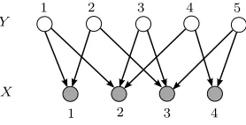
In this section, we consider a fixed sparsity pattern on the population structure A and establish generic identifiability when non-zero entries ofAare drawn from some continuous distribution. Before providing the main result, a generalized notion of (perfect) matching for bipartite graphs is defined. We subsequently impose these conditions on the bipartite graph from topics to words which encodes the sparsity pattern of population structureA.

3.1.1 Generalized Matching for Bipartite Graphs

A bipartite graph with two disjoint vertex sets Y and X and an edge set E between them is denoted byG(Y, X;E). Given the bi-adjacency matrixA, the notationG(Y, X;A) is also used to denote a bipartite graph. Here, the rows and columns of matrix A ∈R|X|×|Y| _are respectively indexed byXand Y vertex sets. For any subsetS_⊆Y, the set of neighbors of vertices in S with respect to A is defined as NA(S) :={i∈X :Aij 6= 0 for some j∈S},

or equivalently,NE(S) :={i∈X: (j, i)∈E for some j ∈S} with respect to edge setE.

Here, we define a generalized notion of matching for a bipartite graph and refer to it as n-gram matching.

Definition 4 ((Perfect) n-gram matching) An-gram matchingM for a bipartite graph

G(Y, X;E) is a subset of edges M ⊆ E which satisfies the following conditions. First, for any j _∈ Y, we have _|NM(j)| ≤ n. Second, for any j1, j2 ∈ Y, j1 6= j2, we have

min_{|NM(j1)|,|NM(j2)|}>|NM(j1)∩NM(j2)|.

A perfect n-gram matching or Y-saturating n-gram matching for the bipartite graph

G(Y, X;E) is a n-gram matching M in which each vertex in Y is exactly connected to n

edges in M.

In words, in a n-gram matching M, each vertex j _∈ Y is at most connected to n edges in M and for any pair of vertices in Y (j1, j2 ∈Y, j1 6=j2), there exists at least one

non-common neighbor in setX for each of them (j1 and j2).

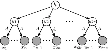
As an example, a bipartite graph G(Y, X;E) with _|X_| = 4 and _|Y_| = 6 is shown in Figure 2 for which the edge setE itself is a perfect 2-gram matching.

We also define the following definition of a n-gram matrix.

Definition 5 (n-gram Matrix) Given a matrix A ∈ Rp×q_{, its} _n_{-gram matrix} _An _∈ Rpn_×_q

is defined as the matrix whose(i, j)-th entry is given by, fori:= (i1, i2, . . . , in)∈[p]n and j_∈[q],

An(i, j) :=Ai1,jAi2,j· · ·Ain,j, or A n_:=

ntimes

z }| {

(14)

Anandkumar, Hsu, Janzamin and Kakade When are Overcomplete Topic Models Identifiable?

Y

X

Figure 2: A bipartite graphG(Y, X;E) with|X|= 4 and|Y|= 6 where the edge set Eitself is a perfect 2-gram matching.

Definition 3 (Canonical form) Population structure A is said to be in canonical form if all of its columns have unit norm.

3.1 Deterministic Conditions for Generic Identifiability

In this section, we consider a fixed sparsity pattern on the population structure A and establish generic identifiability when non-zero entries ofAare drawn from some continuous distribution. Before providing the main result, a generalized notion of (perfect) matching for bipartite graphs is defined. We subsequently impose these conditions on the bipartite graph from topics to words which encodes the sparsity pattern of population structureA.

3.1.1 Generalized Matching for Bipartite Graphs

A bipartite graph with two disjoint vertex setsY andX and an edge set E between them is denoted byG(Y, X;E). Given the bi-adjacency matrix A, the notationG(Y, X;A) is also used to denote a bipartite graph. Here, the rows and columns of matrixA ∈R|X|×|Y| _are

respectively indexed byX andY vertex sets. For any subsetS ⊆Y, the set of neighbors of vertices in S with respect to A is defined asNA(S) :={i ∈X :Aij #= 0 for some j ∈S}, or equivalently, NE(S) :={i∈X: (j, i)∈E for some j∈S}with respect to edge set E.

Here, we define a generalized notion of matching for a bipartite graph and refer to it as n-gram matching.

Definition 4 ((Perfect) n-gram matching) An-gram matchingM for a bipartite graph G(Y, X;E) is a subset of edges M _⊆ E which satisfies the following conditions. First, for any j _∈ Y, we have _|NM(j)| ≤ n. Second, for any j1, j2 ∈ Y, j1 #= j2, we have min{|NM(j1)|,|NM(j2)|}>|NM(j1)∩NM(j2)|.

A perfect n-gram matching or Y-saturating n-gram matching for the bipartite graph G(Y, X;E) is a n-gram matching M in which each vertex in Y is exactly connected to n edges in M.

In words, in a n-gram matching M, each vertex j ∈ Y is at most connected to n edges in M and for any pair of vertices inY (j1, j2 ∈Y, j1 #=j2), there exists at least one non-common neighbor in setX for each of them (j1 andj2).

As an example, a bipartite graph G(Y, X;E) with _|X_| = 4 and _|Y_| = 6 is shown in Figure 2 for which the edge setE itself is a perfect 2-gram matching.

We also define the following definition of an-gram matrix.

Definition 5 (n-gram Matrix) Given a matrix A ∈ Rp×q_{, its} _n_{-gram matrix} _A"n _∈

Rpn_×_q

is defined as the matrix whose(i, j)-th entry is given by, fori:= (i1, i2, . . . , in)∈[p]n 13

Figure 2: A bipartite graphG(Y, X;E) with |X|= 4 and |Y|= 6 where the edge setE itself is a perfect 2-gram matching.

That is,Anis the column-wisenth _{order Kronecker product of}_n_{copies of}_A_{, and is known} as the Khatri-Rao product (Golub and Loan, 2012). Given bipartite graph G(Y, X;A), the notation G(Y, X(n)_;_An_{) is also used to denote the bipartite graph corresponding to}

bi-adjacency matrix An. HereX(n) denotes all orderedn-tuples generated from elements of setX which indexes the rows of An.

The above two definitions might seem unrelated at the first glance, but the following lemma connects them where an interesting property is stated relating the existence of perfect matching in G(Y, X(n);An) to the existence of perfect n-gram matching in G(Y, X;A). This property is also the original motivation behind defining such notion of generalized matching.

Lemma 1 IfG(Y, X;A)has a perfectn-gram matching, thenG(Y, X(n)_;_An₎_{has a perfect} matching. In the other direction, if G(Y, X(n);An) has a perfect matching Mn, then

G(Y, X;A) has a perfect n-gram matching under the following condition on Mn. All the matching edges (j,(i1, . . . , in))∈ Mn should satisfy i1 6= i2 6= · · · 6= in for all j ∈ Y. In words, the matching edges should be connected to nodes inX(n), which are indexed by tuples of distinct indices.

See Appendix A.4 for the proof.

We also provide more discussions and remarks on the n-gram matching as follows.

Remark 6 (Relationship to other matchings) The relationship of n-gram matching to other types of matchings is discussed below.

• Regular matching: For special case n = 1, the (perfect) n-gram matching reduces to the usual (perfect) matching for bipartite graphs.

• b-matching: For a bipartite graph G(Y, X;E), a b-matching for vertices in Y is a subset of edges Mb ⊆E, where each vertex in Y is connected to b edges. Comparing with the proposed perfect (Y-saturating)b-gram matching,b-matching does not enforce that the set of neighbors be different.

Remark 7 (Necessary size bound) Consider a bipartite graphG(Y, X;E) with|Y|=q

and_|X_|=pwhich has a perfectn-gram matching. Note that there are _npn-combinations on

Xside and each combination can at most have one neighbor (a node inY which is connected to all nodes in the combination) through the matching, and therefore we necessarily have

(15)

Finally, note that the existence of perfect n-gram matching results in the existence of perfect (n+1)-gram matching8, but the reverse is not true. For example, the bipartite graph G(Y, X;E) with_|X_|= 4 and_|Y_|= 4₂= 6 in Figure 2, has a perfect 2-gram matching, but not a perfect (1-gram) matching (since 6>4).

3.1.2 Identifiability Conditions Based on Existence of Perfect n-gram

Matching in Topic-word Graph

Now, we are ready to propose the identifiability conditions and result.

Condition 2 (Perfect n-gram matching on A) The bipartite graphG(Vh, Vo;A)between hidden and observed variables, has a perfect n-gram matching9.

The above condition implies that the sparsity pattern of matrix A is appropriately scattered in the mapping from hidden to observed variables to be identifiable. Intuitively, it means that every hidden node can be distinguished from another hidden node by its unique set of neighbors under the corresponding n-gram matching.

Furthermore, condition 2 is the key to be able to propose identifiability in the overcom-plete regime. As stated in the size bound in Remark 7, for n _≥ 2, the number of hidden variables can be more than the number of observed variables and we can still have perfect n-gram matching.

Definition 8 (Kruskal rank, (Kruskal, 1977)) The Kruskal rankor the krankof ma-trix A is defined as the maximum number k such that every subset of k columns of A is linearly independent.

Note that krank is different from the general notion of matrix rank and it is a lower bound for the matrix rank, i.e., Rank(A)≥krank(A).

Condition 3 (Krank condition on A) The Kruskal rank of matrixAsatisfies the bound

krank(A)≥dmax(A)n, where dmax(A)is the maximum node degree of any column ofA, i.e.,

dmax(A) := maxi∈[q]kAeik0. Heren is the same as parametern in Condition 2.

In the overcomplete regime, it is not possible forAto be full column rank and krank(A)<

|Vh|=q. However, note that a large enough krank ensures that appropriate sized subsets of

columns ofAare linearly independent. For instance, when krank(A)>1, any two columns cannot be collinear and the above condition rules out the collinear case for identifiability. In the above condition, we see that a larger krank can incorporate denser connections between topics and words.

On the other hand, the bound in Condition 3 imposes sparsity on the columns of topic-word matrix asdmax(A)≤krank(A)1/n. Under such sparsity constraint, each topic (index-8. Note that the degree of each node (on matching sideY) in the original bipartite graph should be at least

n+ 1.

(16)

ing the columns ofA) is supported on a specific set of words which enables us to distinguish between different topics and identify the model. But, it seems that this bound is not tight10. The main identifiability result under a fixed graph structure is stated in the following theorem forn_≥2, wherenis the topic persistence level. The identifiability result relies on having access to the (2rn)-th order moment of observed variables xl, l ∈ [2rn], defined in

equation (2) as

M2rn(x) :=E h

∈Rprn_×_prn ,

for some integerr ≥1.

Theorem 9 (Generic identifiability under deterministic topic-word graph structure) LetM₂(n_rn)(x)in equation (2)be the(2rn)-th order observed moment of the n-persistent topic model for some integer r _≥ 1. If the model satisfies conditions 1, 2 and 3, then, for any

n_≥2, all the columns of population structureA are generically identifiablefrom M₂(_rnn)(x). Furthermore, the (2r)-th order moment of the hidden variables, denoted by M2r(h), is also

generically identifiable.

The theorem is proved in Appendix A. It is seen that the population structure A is iden-tifiable, given any observed moment of order at least 2n. Increasing the order of observed moment results in identifying higher order moments of the hidden variables.

The above theorem does not cover the case when the persistence leveln= 1. This is the usual bag-of-words admixture model. Identifiability of this model has been studied earlier in Anandkumar et al. (2012) and we recall it below.

Remark 10 (Bag-of-words admixture model, (Anandkumar et al., 2012)) Given(2r) -th order observed moments wi-th r≥1, the structure of the popular bag-of-words admixture model and the (2r)-th order moment of hidden variables are identifiable, when A is full column rank and the following expansion condition holds (Anandkumar et al., 2012)

|NA(S)| ≥ |S|+dmax(A), ∀S ⊆Vh, |S| ≥2. (4) Our result for n≥2 in Theorem 9, provides identifiability in the overcomplete regime with weaker matching condition 2 and krank condition 3. The matching condition 2 is weaker than the above expansion condition which is based on the perfect matching and hence, does not allow overcomplete models. Furthermore, the above result for the bag-of-words admixture model requires full column rank of A which is more stringent than our krank condition 3.

Remark 11 (Kruskal rank and degree diversity) Condition 3 requires that the Kruskal rank of the topic-word matrix be large enough compared to the maximum degree of the top-ics. Intuitively, a larger Kruskal rank ensures enough diversity in the word supports among different topics under a higher level of sparsity. This Kruskal rank condition also allows for more degree diversity among the topics, when the topic persistence level n > 1. On

10. The looseness originates from bound (37) as

NA_Rest.n (S)

≥ |NA(S)|+|S| in the proof. See

Defini-tions 5 and 25 for the definition ofA_Restn _.. Note that many terms in this lower bound on

NA_Rest.n (S)

(17)

the other hand, for the bag-of-words model (n = 1), using (4) implies that 2dmin > dmax, where dmin, dmax are the minimum and maximum degrees of the topics. Thus, we provide identifiability results with more degree diversity when higher order moments are employed.

Remark 12 (Recovery using `1 optimization) It turns out that our conditions for iden-tifiability imply that the columns of then-gram matrix An, defined in Definition 5, are the sparsest vectors in ColM₂(n_n)(x), having a tensor rank of one. See Appendix A. This im-plies recovery of the columns of A through exhaustive search, which is not efficient. On the other hand, efficient `1-based recovery algorithms have been analyzed in Spielman et al. (2012a); Anandkumar et al. (2012) for the undercomplete case (n= 1). They can be em-ployed here for recovery from higher order moments as well. Exploiting additional structure present in An_{, for} _{n >} ₁_{, such as rank-1 test devices proposed in De Lathauwer et al.} (2007) are interesting avenues for future investigation.

In Theorem 9, we provide our identifiability result for the overcomplete topic-word matrix A under topic persistent model. The result for the bag-of-words admixture model is also reviewed in Remark 10 under the assumption that A is full column rank. In the following corollary, we provide the strong identifiability result for the full column rank topic-word matrix under the topic persistent model.

Corollary 13 (Identifiability for undercomplete topic-word matrix) LetM₂(n_rn)(x)in equation (2)be the (2rn)-th order observed moment of then-persistent topic model for some integer r _≥ 1. If the model satisfies condition 1, and in addition A is full column rank, then for any n _≥ 2, all the columns of population structure A are generically identifiable

from M₂(_rnn)(x). Furthermore, the (2r)-th order moment of the hidden variables, denoted by

M2r(h), is also generically identifiable.

Comparing to Theorem 9 and Remark 10, the expansion (and krank) conditions are not required in the above result which is a huge relaxation. The reason is both undercomplete regime and topic persistence are assumed here which relaxes the other conditions. Note that the assumptions that topic persists with persistencen≥2, and the topic-word matrix is full column rank (and therefore undercomplete) is reasonable in many applications.

3.2 Analysis Under Random Topic-word Graph Structures

In this section, we specialize the identifiability result to the random case. This result is based on more transparent conditions on the size and the degree of the random bipartite graph G(Vh, Vo;A). We consider the random model where in the bipartite graph G(Vh, Vo;A),

each node i_∈Vh is randomly connected todi different nodes in setVo. Note that this is a

heterogeneous degree model.

Furthermore, the random identifiability result is provided with high probability which is defined as follows.

Definition 14 (whp) A sequence of eventsEp(depending on size parameterp) occurs with

high probability(whp) ifPr(_Ep) = 1−O(p−) for some >0.

(18)

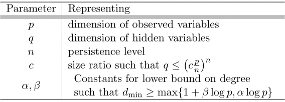
Parameter Representing

p dimension of observed variables q dimension of hidden variables n persistence level

c size ratio such thatq ≤ c_npn

α, β Constants for lower bound on degree such thatdmin ≥max{1 +βlogp, αlogp}

Table 1: Table of parameters.

This size condition is required to establish that the random bipartite graph has a perfect n-gram matching (and hence satisfies deterministic condition 2). It is shown in Section 5.2.1 that the necessary size constraint q = O(pn) stated in Remark 7, is achieved in the random case. Thus, the above constraint allows for the overcomplete regime, where q p forn_≥2, and is tight.

Condition 5 (Degree condition) In the random bipartite graphG(Vh, Vo;A) with|Vh|= q,|Vo| =p, and A ∈Rp×q, the degree di of nodes i ∈ Vh satisfies the following lower and upper bounds (di∈[dmin, dmax]):

• Lower bound: dmin ≥ max{1 +βlogp, αlogp} for some constants β > _{log 1}n−1_/c, α >

max2n2 _β_log1 c + 1

,2βn .

• Upper bound: dmax≤(cp)

1

n.

Intuitively, the lower bound on the degree is required to show that the corresponding bi-partite graph G(Vh, Vo;A) has sufficient number of random edges to ensure that it has

perfect n-gram matching with high probability. The upper bound on the degree is mainly required to satisfy the krank condition 3, where dmax(A)n ≤krank(A). As discussed after

Condition 3, this upper bound is not tight.

It is important to see that, for n≥2, the above condition on degree covers a range of models from sparse to intermediate regimes and it is reasonable in a number of applications that each topic does not generate a very large number of words.

The proposed parameters in Conditions 4 and 5 are summarized in Table 1.

The main random identifiability result is stated in the following theorem forn≥2, while n= 1 case is addressed in Remark 17. The identifiability result relies on having access to the (2rn)-th order moment of observed variables xl, l∈[2rn], defined in equation (2) as

M2rn(x) :=E h

∈Rprn_×_prn ,

for some integerr ≥1.

Probability rate constants: The probability rate of success in the following random iden-tifiability result is specified by constantsβ0 >0 and γ =γ1+γ2 >0 as

(19)

γ1 =en−1

_c

nn−1 +

e2 1₋δ1

nβ0+1, (6)

γ2 =

cn−1e2 nn₍₁₋_δ

2)

, (7)

where δ1 and δ2 are some constants satisfying e2

p n

−βlog 1/c

< δ1 < 1 and c n−1_e2

nn p−β 0

< δ2 <1.

Theorem 15 (Random identifiability) LetM₂(n_rn)(x) in equation (2) be the(2rn)-th or-der observed moment of the n-persistent topic model for some integer r ≥1. If the model with random population structure A satisfies conditions 1, 4 and 5, then whp (with proba-bility at least 1₋γp−β0 _{for constants}_β0 _>₀ _and_{γ >}₀_{, specified in} ₍₅₎_-₍₇₎_{), for any}_n_≥₂_,

all the columns of population structure A are identifiable from M₂(n_rn)(x). Furthermore, the

(2r)-th order moment of hidden variables, denoted byM2r(h), is also identifiable, whp.

The theorem is proved in Appendix B. Similar to the deterministic analysis, it is seen that the population structure A is identifiable given any observed moment with order at least 2n. Increasing the order of observed moment results in identifying higher order mo-ments of the hidden variables.

Remark 16 (Trade-off between topic-word size ratio and degree) When the num-ber of hidden variables increases, i.e. c increases, but the order n is kept fixed, the bounds on degree in condition 5 also needs to grow. Intuitively, a larger degree is needed to provide more flexibility in choosing the subsets of neighbors for hidden nodes to ensure the existence of a perfect n-gram matching in the bipartite graph, which in turn ensures identifiability. Note that as c grows, the parameter β, which is the lower bound on dalso grows, and the probability rate (i.e., the term −βlogc) remains constant. Hence, the probability rate does not change as c increases, since the increase in the degree d compensates the additional “difficulty” arising due to a larger number of hidden variables.

The above identifiability theorem only covers forn≥2 and then= 1 case is addressed in the following remark.

Remark 17 (Bag-of-words admixture model) The identifiability result for the ran-dom bag-of-words admixture model is comparable to the result in Spielman et al. (2012a), which considers exact recovery of sparsely-used dictionaries. They assume that Y = DX

is given for some unknown arbitrary dictionary D _∈ Rq×q and unknown random sparse coefficient matrix X _∈_Rq×p_{. They establish that if} _D _∈_Rq×q _{is full rank and the random} sparse coefficient matrix X ∈Rq×p _{follows the Bernoulli-subgaussian model with size} con-straint p > Cqlogq and degree constraint O(logq) < E[d]< O(qlogq), then the model is identifiable, whp. Comparing the size and degree constraints, our identifiability result for

(20)

Remark 18 (The size condition is tight) The size boundq=O(pn₎ _{in the above} theo-rem achieves the necessary condition thatq≤ _np=O(pn) (see Remark 7), and is therefore tight. The sufficiency is argued in Theorem 22, where we show that the matching condition 2 holds under the above size and degree conditions 4 and 5.

As in the deterministic case, we finish this section by providing random identifiability result for the full column rank topic-word matrix under the topic persistent model.

Corollary 19 (Random identifiability for undercomplete topic-word matrix) Let

M₂(_rnn)(x) in equation (2) be the (2rn)-th order observed moment of the n-persistent topic model for some integer r _≥ 1. If the model with random population structure A _∈ Rp×q

satisfies condition 1, size condition q _≤ cp for some constant 0 < c < 1 and the degree condition dmin ≥1 +βlogp for some constant β > 0, then whp (with probability at least

1₋O(z−βlog 1/c)whereβlog1_c >0), for anyn_≥2, all the columns of population structureA

are identifiable from M₂(n_rn)(x). Furthermore, the(2r)-th order moment of hidden variables, denoted by M2r(h), is also identifiable, whp.

Comparing to Theorem 15, the upper bound on the degree (sparsity constraint) is not required in the above result which is a huge relaxation.

4. Identifiability via Uniqueness of Tensor Decompositions

In this section, we characterize the moments of the n-persistent topic model in terms of the model parameters, i.e. the topic-word matrix A and the moment of hidden variables. We relate identifiability of the topic model to uniqueness of a certain class of tensor de-compositions, which in turn, enables us to prove Theorems 9 and 15. We then discuss the special cases of the persistent topic model, viz., the single topic model (infinite-persistent topic model) and the bag-of-words admixture model (1-persistent topic model).

4.1 Moment Characterization of the Persistent Topic Model

In the following lemma, which is proved in Appendix A.2, we characterize the observed moments of a persistent topic model. Throughout this section, the order of the observed moment is fixed to 2m.

Lemma 2 (n-persistent topic model moment characterization) The (2m)-th order moment of observed variables, defined in equation (2), for the n-persistent topic model is characterized as11:

• if m=rn, for some integer r≥1, then

M₂(_mn)(x) =

r times

z }| {

An⊗ · · · ⊗An

M2r(h)

r times

z }| {

An⊗ · · · ⊗An _>

, (8)

where M2r(h) ∈ Rq r_×_qr

is the (2r)-th order moment of hidden variables h _∈ Rq, defined in equation (3), and then-gram matrix An _{is defined in Definition 5.}

(21)

h

y

x1 xm xm+1 x2m

(a) Single topic model

(infinite-persistent topic model)

h

y1 ym ym+1 y2m

x1 xm xm+1 x2m

(b) Bag-of-words admixture model (1-persistent topic model)

Figure 3: Hierarchical structure of the single topic model and bag-of-words admixture model shown for 2mnumber of words (views).

the persistence level is large enough compared to the order of the moment (n≥ 2m), the moment form reduces to a Khatri-Rao product form in (9). Moreover, in (9), we have a diag-onal matrixM1(h) instead of a general (dense) matrixM2r(h) in (8), whenn <2m= 2rn. Thus, we have a more succinct representation of the moments in (9) when the persistence level of the topics is large enough.

In the following, we contrast the special cases when the persistence level n is n → ∞

(single topic model) and n = 1 (bag of words admixture model), as shown in Fig.3a and Fig.3b. In order to have a fair comparison, the number of observed variables is fixed to 2m and the persistence level is varied.

Single topic model (n→ ∞): The condition in (9) (n≥2m) is always satisfied for the single-topic model, since n→ ∞in this case, and we have

M2(∞m)(x) = !

A"m"M1(h)!A"m"#. (10)

Note that M1(h) is a diagonal matrix.

Bag-of-words admixture model (n= 1): From Lemma 2, the (2m)-th order moment of observed variables xl, l ∈ [2m], for the bag-of-words admixture model (1-persistent topic model), shown in Figure 3b, is given by

M₂(1)_m(x) =#

mtimes $ %& '

A⊗ · · · ⊗A(M2m(h)

#$ mtimes%& '

A⊗ · · · ⊗A(#, (11)

where M2m(h)∈Rq m_×_qm

is the (2m)-th order moment of hidden variables h∈Rq, defined in (3). Note thatM2m(h) is a full matrix in general.

Contrasting single topic (n → ∞) and bag of words models (n = 1): Comparing equa-tions (10) and (11), it is seen that the moments under the single topic model in (10) are more “structured” compared to the bag of words model in (11). In (11), we have Kronecker products of the topic-word matrix A, while (10) involves Khatri-Rao products of A. This forms a crucial criterion in determining of whether overcomplete models are identifiable, as discussed below.

Why does persistence help in identifiability of overcomplete models? For simplicity, let the order of the moment 2m= 4. The equations (10) and (11) reduce to

M₄(∞)(x) = (A&A) Diag!_E)h]"(A&A)#, (12)

21 (a) Single topic model

(infinite-persistent topic model) h

y

x1 xm xm+1 x2m

(a) Single topic model

(infinite-persistent topic model)

h

y1 ym ym+1 y2m

x1 xm xm+1 x2m

the persistence level is large enough compared to the order of the moment (n_≥ 2m), the moment form reduces to a Khatri-Rao product form in (9). Moreover, in (9), we have a diag-onal matrix M1(h) instead of a general (dense) matrixM2r(h) in (8), whenn <2m= 2rn. Thus, we have a more succinct representation of the moments in (9) when the persistence level of the topics is large enough.

In the following, we contrast the special cases when the persistence level n is n_{→ ∞} (single topic model) and n = 1 (bag of words admixture model), as shown in Fig.3a and Fig.3b. In order to have a fair comparison, the number of observed variables is fixed to 2m and the persistence level is varied.

Single topic model (n→ ∞): The condition in (9) (n≥ 2m) is always satisfied for the single-topic model, since n_{→ ∞}in this case, and we have

M₂(∞_m)(x) =!A"m"M1(h)!A"m"#. (10) Note that M1(h) is a diagonal matrix.

Bag-of-words admixture model (n= 1): From Lemma 2, the (2m)-th order moment of observed variables xl, l ∈ [2m], for the bag-of-words admixture model (1-persistent topic model), shown in Figure 3b, is given by

M₂(1)_m(x) =#

mtimes $ %& '

A_{⊗ · · · ⊗}A(M2m(h)

#$ mtimes%& '

A_{⊗ · · · ⊗}A(#, (11)

whereM2m(h)∈Rq m_×_qm

is the (2m)-th order moment of hidden variables h_∈_Rq_{, defined} in (3). Note thatM2m(h) is a full matrix in general.

Contrasting single topic (n→ ∞) and bag of words models (n= 1): Comparing equa-tions (10) and (11), it is seen that the moments under the single topic model in (10) are more “structured” compared to the bag of words model in (11). In (11), we have Kronecker products of the topic-word matrix A, while (10) involves Khatri-Rao products of A. This forms a crucial criterion in determining of whether overcomplete models are identifiable, as discussed below.

M₄(∞)(x) = (A_&A) Diag!_E)h]"(A_&A)#, (12)

21

• If n_≥2m, then

M₂(_mn)(x) = AmM1(h) Am

_>

, (9)

where M1(h) := Diag(E[h]) ∈ Rq×q is the first order moment of hidden variables

h_∈Rq, stacked in a diagonal matrix.

Thus, we see that the observed moments can be expressed in terms of the hidden mo-mentsM(h) and the Kronecker products of then-gram matrices. In the special case, when the persistence level is large enough compared to the order of the moment (n_≥ 2m), the moment form reduces to a Khatri-Rao product form in (9). Moreover, in (9), we have a diag-onal matrixM1(h) instead of a general (dense) matrixM2r(h) in (8), when n <2m= 2rn.

Thus, we have a more succinct representation of the moments in (9) when the persistence level of the topics is large enough.

In the following, we contrast the special cases when the persistence level n is n → ∞ (single topic model) and n= 1 (bag of words admixture model), as shown in Fig.3a and Fig.3b. In order to have a fair comparison, the number of observed variables is fixed to 2m and the persistence level is varied.

Single topic model (n_{→ ∞}): The condition in (9) (n_≥2m) is always satisfied for the single-topic model, since n_{→ ∞} in this case, and we have

M₂(_m∞)(x) = AmM1(h) Am>. (10)

Note thatM1(h) is a diagonal matrix.

Bag-of-words admixture model (n= 1): From Lemma 2, the (2m)-th order moment of observed variables xl, l ∈ [2m], for the bag-of-words admixture model (1-persistent topic

model), shown in Figure 3b, is given by

M₂(1)_m(x) =

mtimes

z }| {

A_{⊗ · · · ⊗}AM2m(h)

z mtimes}| {

A_{⊗ · · · ⊗}A>, (11)

whereM2m(h)∈Rq m_×_qm

is the (2m)-th order moment of hidden variables h∈Rq_{, defined}

(22)

Contrasting single topic (n_{→ ∞}) and bag of words models (n= 1): Comparing equa-tions (10) and (11), it is seen that the moments under the single topic model in (10) are more “structured” compared to the bag of words model in (11). In (11), we have Kronecker products of the topic-word matrix A, while (10) involves Khatri-Rao products of A. This forms a crucial criterion in determining of whether overcomplete models are identifiable, as discussed below.

M₄(∞)(x) = (AA) Diag Eh](AA)>, (12) M₄(1)(x) = (A⊗A)E(h⊗h)(h⊗h)>(A⊗A)>. (13) Note that for the single topic model in (12), the Khatri-Rao product matrixAA∈Rp2_×_q has the same as the number of columns (i.e. the latent dimensionality) of the original matrix A, while the number of rows (i.e. the observed dimensionality) is increased. Thus, the Khatri-Rao product “expands” the effect of hidden variables to higher order observed variables, which is the key towards identifying overcomplete models. In other words, the original overcomplete representation becomes determined due to the ‘expansion effect’ of the Khatri-Rao product structure of the higher order observed moments.

On the other hand, in the bag-of-words admixture model in (13), this interesting ‘expan-sion property’ does not occur, and we have the Kronecker productA_⊗A_∈_Rp2_×_q2

, in place of the Khatri-Rao products. The Kronecker product operation increases both the number of the columns (i.e. latent dimensionality) and the number of rows (i.e. observed dimen-sionality), which implies that higher order moments do not help in identifying overcomplete models.

An example is provided in Figure 4 which helps to see how the matrices AA and A_⊗A behave differently in terms of mapping topics to word tuples.

Note that for the n-persistent model, for n= 2, the 4th _{order moment reduces to}

M₄(2)(x) = (AA)Ehh>](AA)>. (14) Contrasting the above equation with (12) and (13), we find that the 2-persistent model retains the desirable property of possessing Khatri-Rao products, while being more general than the form for single topic model in (12). This key property enables us to establish identifiability of topic models with finite persistence levels.

4.2 Tensor Algebra of the Moments

In Section 4.1, we provided a representation of the moment forms in the matrix form. We now provide the equivalent tensor representation of the moments. The tensor representation is more compact and transparent, and allows us to compare the topic models under different levels of persistence. We compare the derived tensor form with the well-known Tucker and CP decompositions. We first introduce some tensor notations and definitions.

4.2.1 Tensor Notations and Definitions

A real-valued order-n tensor A ∈ Nni=1Rpi := Rp1×···×pn is a n dimensional array A(1 :