An Interior-Point Method for Large-Scale
`
1-Regularized
Logistic Regression
Kwangmoo Koh [email protected]
Seung-Jean Kim [email protected]
Stephen Boyd [email protected]
Information Systems Laboratory Electrical Engineering Department Stanford University
Stanford, CA 94305-9510, USA
Editor: Yi Lin
Abstract
Logistic regression with `1 regularization has been proposed as a promising method for feature selection in classification problems. In this paper we describe an efficient interior-point method for solving large-scale`1-regularized logistic regression problems. Small problems with up to a thousand or so features and examples can be solved in seconds on a PC; medium sized problems, with tens of thousands of features and examples, can be solved in tens of seconds (assuming some sparsity in the data). A variation on the basic method, that uses a preconditioned conjugate gradient method to compute the search step, can solve very large problems, with a million features and ex-amples (e.g., the 20 Newsgroups data set), in a few minutes, on a PC. Using warm-start techniques, a good approximation of the entire regularization path can be computed much more efficiently than by solving a family of problems independently.
Keywords: logistic regression, feature selection,`1regularization, regularization path, interior-point methods.
1. Introduction
In this section we describe the basic logistic regression problem, the`2- and`1-regularized versions,
and the regularization path. We set out our notation, and review existing methods and literature. Finally, we give an outline of this paper.
1.1 Logistic Regression
Let x∈Rndenote a vector of explanatory or feature variables, and b∈ {−1,+1}denote the associ-ated binary output or outcome. The logistic model has the form
Prob(b|x) = 1
1+exp(−b(wTx+v)) =
exp b(wTx+v) 1+exp(b(wTx+v)),
where Prob(b|x)is the conditional probability of b, given x∈Rn. The logistic model has parameters
v∈R (the intercept) and w∈Rn(the weight vector). When w6=0, wTx+v=0 defines the neutral
the conditional probability of outcome b=1 is 1/(1+1/e)≈0.73, and the conditional probability of b=−1 is 1/(1+e)≈0.27. On the hyperplane wTx+v=−1, these conditional probabilities are reversed. As wTx+v increases above one, the conditional probability of outcome b=1 rapidly approaches one; as wTx+v decreases below −1, the conditional probability of outcome b=−1 rapidly approaches one. The slab in feature space defined by|wTx+v| ≤1 defines the ambiguity
region, in which there is substantial probability of each outcome; outside this slab, one outcome is
much more likely than the other.
Suppose we are given a set of (observed or training) examples,
(xi,bi)∈Rn× {−1,+1}, i=1, . . . ,m,
assumed to be independent samples from a distribution. We use plog(v,w)∈Rmto denote the vector
of conditional probabilities, according to the logistic model,
plog(v,w)i=Prob(bi|xi) =
exp(wTai+vbi)
1+exp(wTa
i+vbi)
, i=1, . . . ,m,
where ai=bixi. The likelihood function associated with the samples is ∏i=m1plog(v,w)i, and the
log-likelihood function is given by
m
∑
i=1
log plog(v,w)i=− m
∑
i=1
f(wTai+vbi),
where f is the logistic loss function
f(z) =log(1+exp(−z)). (1)
This loss function is convex, so the likelihood function is concave. The negative of the log-likelihood function is called the (empirical) logistic loss, and dividing by m we obtain the average
logistic loss,
lavg(v,w) = (1/m) m
∑
i=1
f(wTai+vbi).
We can determine the model parameters w and v by maximum likelihood estimation from the observed examples, by solving the convex optimization problem
minimize lavg(v,w), (2)
with variables v∈R and w∈Rn, and problem data A= [a1 · · · am]T∈Rm×nand the vector of binary
outcomes b= [b1 · · · bm]T∈Rm. The problem (2) is called the logistic regression problem (LRP).
The average logistic loss is always nonnegative, that is, lavg(v,w)≥0, since f(z)≥0 for any z.
For the choice w=0, v=0, we have lavg(0,0) =log 2≈0.693, so the optimal value of the LRP
lies between 0 and log 2. In particular, the optimal value can range (roughly) between 0 and 1. The optimal value is 0 only when the original data are linearly separable, that is, there exist w and v such that wTxi+v>0 when bi=1, and wTxi+v<0 when bi =−1. In this case the optimal value of
the LRP (2) is not achieved (except in the limit with w and v growing arbitrarily large). The optimal value is log 2, that is, w=0, v=0 are optimal, only if∑mi=1bi=0 and∑mi=1ai=0. (This follows
examples (i.e., those for which bi=1) is equal to the number of negative examples, and the average
of xiover the positive examples is the negative of the average value of xiover the negative examples.
The LRP (2) is a smooth convex optimization problem, and can be solved by a wide variety of methods, such as gradient descent, steepest descent, Newton, quasi-Newton, or conjugate-gradients (CG) methods (see, for example Hastie et al., 2001, § 4.4).
Once we find maximum likelihood values of v and w, that is, a solution of (2), we can predict the probability of the two possible outcomes, given a new feature vector x∈Rn, using the associated
logistic model. For example, when w6=0, we can form the logistic classifier
φ(x) =sgn(wTx+v), (3)
where
sgn(z) =
+1 z>0 −1 z≤0,
which picks the more likely outcome, given x, according to the logistic model. This classifier is linear, meaning that the boundary between the two decision outcomes is a hyperplane (defined by
wTx+v=0).
1.2 `2-Regularized Logistic Regression
When m, the number of observations or training examples, is not large enough compared to n, the number of feature variables, simple logistic regression leads to over-fit. That is, the classifier found by solving the LRP (2) performs perfectly (or very well) on the training examples, but may perform poorly on unseen examples. Over-fitting tends to occur when the fitted model has many feature variables with (relatively) large weights in magnitude, that is, w is large.
A standard technique to prevent over-fitting is regularization, in which an extra term that pe-nalizes large weights is added to the average logistic loss function. The `2-regularized logistic regression problem is
minimize lavg(v,w) +λkwk22= (1/m)∑mi=1f(wTai+vbi) +λ∑ni=1w2i. (4)
Hereλ>0 is the regularization parameter, used to control the trade-off between the average logistic loss and the size of the weight vector, as measured by the`2-norm. No penalty term is imposed
on the intercept, since it is a parameter for thresholding the weighted sum wTx in the linear
classi-fier (3). The solution of the`2-regularized regression problem (4) (which exists and is unique) can
be interpreted in a Bayesian framework, as the maximum a posteriori probability (MAP) estimate of w and v, when w has a Gaussian prior distribution on Rn with zero mean and covarianceλI and v has the (improper) uniform prior on R; see, for example, Chaloner and Larntz (1989) or Jaakkola
and Jordan (2000).
the author compares several methods for`2-regularized LRPs with large data sets. The fastest
meth-ods turn out to be conjugate-gradients and limited memory Newton methmeth-ods, outperforming IRLS, gradient descent, and steepest descent methods. Truncated Newton methods have been applied to large-scale problems in several other fields, for example, image restoration (Fu et al., 2006) and support vector machines (Keerthi and DeCoste, 2005). For large-scale iterative methods such as truncated Newton or CG, the convergence typically improves as the regularization parameterλis increased, since (roughly speaking) this makes the objective more quadratic, and improves the con-ditioning of the problem.
1.3 `1-Regularized Logistic Regression
More recently, `1-regularized logistic regression has received much attention. The`1-regularized logistic regression problem is
minimize lavg(v,w) +λkwk1= (1/m)∑mi=1f(wTai+vbi) +λ∑ni=1|wi|, (5)
whereλ>0 is the regularization parameter. The only difference with `2-regularized logistic
re-gression is that we measure the size of w by its`1-norm, instead of its`2-norm. A solution of the
`1-regularized logistic regression must exist, but it need not be unique. Any solution of the`1 -regularized logistic regression problem (5) can be interpreted in a Bayesian framework as a MAP estimate of w and v, when w has a Laplacian prior distribution and v has the (improper) uniform prior. The objective function in the`1-regularized LRP (5) is convex, but not differentiable (specif-ically, when any of the weights is zero), so solving it is more of a computational challenge than solving the`2-regularized LRP (4).
Despite the additional computational challenge posed by `1-regularized logistic regression,
compared to`2-regularized logistic regression, interest in its use has been growing. The main moti-vation is that`1-regularized LR typically yields a sparse vector w, that is, w typically has relatively few nonzero coefficients. (In contrast, `2-regularized LR typically yields w with all coefficients
nonzero.) When wj=0, the associated logistic model does not use the jth component of the feature
vector, so sparse w corresponds to a logistic model that uses only a few of the features, that is, components of the feature vector. Indeed, we can think of a sparse w as a selection of the relevant or important features (i.e., those associated with nonzero wj), as well as the choice of the intercept
value and weights (for the selected features). A logistic model with sparse w is, in a sense, sim-pler or more parsimonious than one with nonsparse w. It is not surprising that`1-regularized LR
can outperform`2-regularized LR, especially when the number of observations is smaller than the number of features (Ng, 2004; Wainwright et al., 2007).
We refer to the number of nonzero components in w as its cardinality, denoted card(w). Thus,
`1-regularized LR tends to yield w with card(w)small; the regularization parameterλroughly
con-trols card(w), with largerλtypically (but not always) yielding smaller card(w).
The general idea of `1 regularization for the purposes of model or feature selection (or just
sparsity of solution) is quite old, and widely used in other contexts such as geophysics (Claerbout and Muir, 1973; Taylor et al., 1979; Levy and Fullagar, 1981; Oldenburg et al., 1983). In statistics, it is used in the well-known Lasso algorithm (Tibshirani, 1996) for`1-regularized linear regression,
2001), signal recovery from incomplete measurements (Cand `es et al., 2006, 2005; Donoho, 2006), and wavelet thresholding (Donoho et al., 1995), decoding of linear codes (Cand `es and Tao, 2005), portfolio optimization (Lobo et al., 2005), controller design (Hassibi et al., 1999), computer-aided design of integrated circuits (Boyd et al., 2001), computer vision (Bhusnurmath and Taylor, 2007), sparse principal component analysis (d’Aspremont et al., 2005; Zou et al., 2006), graphical model selection (Wainwright et al., 2007), maximum likelihood estimation of graphical models (Banerjee et al., 2006; Dahl et al., 2005), boosting (Rosset et al., 2004), and`1-norm support vector machines
(Zhu et al., 2004). A recent survey of the idea can be found in Tropp (2006). Donoho and Elad (2003) and Tropp (2006) give some theoretical analysis of why`1regularization leads to a sparse
model in linear regression. Recently, theoretical properties of`1-regularized linear regression have
been studied by several researchers; see, for example, Zou (2006), Zhao and Yu (2006), and Zou et al. (2007).
To solve the`1-regularized LRP (5), generic methods for nondifferentiable convex problems can
be used, such as the ellipsoid method or subgradient methods (Shor, 1985; Polyak, 1987). These methods are usually very slow in practice, however. (Because`1-regularized LR typically results in
a weight vector with (many) zero components, we cannot simply ignore the nondifferentiability of the objective in the`1-regularized LRP (5), hoping to not encounter points of nondifferentiability.)
Another approach is to transform the problem to one with differentiable objective and constraint functions. We can solve the `1-regularized LRP (5), by solving an equivalent formulation, with
linear inequality constraints,
minimize lavg(v,w) +λ1Tu
subject to −ui≤wi≤ui, i=1, . . . ,n,
(6)
where the variables are the original ones v∈R, w∈Rn, along with u∈Rn. Here 1 denotes the vector with all components one, so 1Tu is the sum of the components of u. (To see the equivalence
with the`1-regularized LRP (5), we note that at the optimal point for (6), we must have ui=|wi|,
in which case the objectives in (6) and (5) are the same.) The reformulated problem (6) is a convex optimization problem, with a smooth objective, and linear constraint functions, so it can be solved by standard convex optimization methods such as SQP, augmented Lagrangian, interior-point, and other methods. High quality solvers that can directly handle the problem (6) (and therefore, carry out
`1-regularized LR) include for example LOQO (Vanderbei, 1997), LANCELOT (Conn et al., 1992),
MOSEK (MOSEK ApS, 2002), and NPSOL (Gill et al., 1986). These general purpose solvers can solve small and medium scale`1-regularized LRPs quite effectively.
Other recently developed computational methods for`1-regularized logistic regression include
the IRLS method (Lee et al., 2006; Lokhorst, 1999), a generalized LASSO method (Roth, 2004) that extends the LASSO method proposed in Osborne et al. (2000) to generalized linear models, generalized iterative scaling (Goodman, 2004), bound optimization algorithms (Krishnapuram et al., 2005), online algorithms (Balakrishnan and Madigan, 2006; Perkins and Theiler, 2003), coordinate descent methods (Friedman et al., 2007; Genkin et al., 2006), and the Gauss-Seidel method (Shevade and Keerthi, 2003). Some of these methods can handle very large problems (assuming some sparsity in the data) with modest accuracy. But the additional computational cost required for these methods to achieve higher accuracy can be very large.
The main goal of this paper is to describe a specialized interior-point method for solving the`1
large-scale methods (conjugate-gradients and limited memory Newton) applied to the`2-regularized
LRP.
Numerical experiments show that our method is as fast as, or faster than, other methods, and reliably provides very accurate solutions. Compared with high-quality implementations of general purpose primal-dual interior-point methods, our method is far faster, especially for large problems. Compared with first-order methods such as coordinate descent methods, our method is comparable in solving large problems with modest accuracy, but is able to solve them with high accuracy with relatively small additional computational cost.
In this paper we focus on methods for solving the `1-regularized LRP; we do not discuss the benefits or advantages of`1-regularized LR, compared to `2-regularized LR or other methods for
modeling or constructing classifiers for two-class data.
1.4 Regularization Path
Let(v?λ,w?λ)be a solution for the`1-regularized LRP with regularization parameterλ. The family of
solutions, asλvaries over(0,∞), is called the (`1-) regularization path. In many applications, the
regularization path (or some portion) needs to be computed, in order to determine an appropriate value ofλ. At the very least, the`1-regularized LRP must be solved for multiple, and often many,
values ofλ.
In`1-regularized linear regression, which is the problem of minimizing
kFz−gk2
2+λkzk1
over the variable z, whereλ>0 is the regularization parameter, F ∈Rp×n is the covariate matrix, and g∈Rp is the vector of responses, it can be shown that the regularization path is piecewise linear, with kinks at each point where any component of the variable z transitions from zero to nonzero, or vice versa. Using this fact, the entire regularization path in a (small or medium size)`1
-regularized linear regression problem can be computed efficiently (Hastie et al., 2004; Efron et al., 2004; Rosset, 2005; Rosset and Zhu, 2007; Osborne et al., 2000). These methods are related to numerical continuation techniques for following piecewise smooth curves, which have been well studied in the optimization literature (Allgower and Georg, 1993).
Path following methods have been applied to several problems (Hastie et al., 2004; Park and Hastie, 2006a,b; Rosset, 2005). Park and Hastie (2006a) describe an algorithm for (approximately) computing the entire regularization path for general linear models (GLMs) including logistic re-gression models. In Rosset (2005), a general path-following method based on a predictor-corrector method is described for general regularized convex loss minimization problems. Path-following methods can be slow for large-scale problems, where the number of kinks or events is very large (at least n). When the number of kinks on the portion of the regularization path of interest is modest, however, these path-following methods can be very fast, requiring just a small multiple of the effort needed to solve one regularized problem to compute the whole path (or a portion).
regularization path, much more efficiently than by solving a family of the problems independently. Our method is far more efficient than path following methods in computing a good approximation of the regularization for a medium-sized or large data set.
1.5 Outline
In Section 2, we give (necessary and sufficient) optimality conditions, and a dual problem, for the
`1-regularized LRP. Using the dual problem, we show how to compute a lower bound on the
subopti-mality of any pair(v,w). We describe our basic interior-point method in Section 3, and demonstrate its performance in Section 4 with small and medium scale synthetic and machine learning bench-mark examples. We show that`1-regularized LR can be carried out within around 35 or so iterations,
where each iteration has the same complexity as solving an`2-regularized linear regression problem.
In Section 5, we describe a variation on our basic method that uses a preconditioned conjugate gradient approach to compute the search direction. This variation on our method can solve very large problems, with a million features and examples (e.g., the 20 Newsgroups data set), in under an hour, on a PC, provided the data matrix is sufficiently sparse.
In Section 6, we consider the problem of computing the regularization path efficiently, at a variety of values ofλ(but potentially far fewer than the number of kinks on the path). Using warm-start techniques, we show how this can done much more efficiently than by solving a family of problems independently. In Section 7, we compare the interior-point method with several existing methods for `1-regularized logistic regression. In Section 8, we describe generalizations of our method to other`1-regularized convex loss minimization problems.
2. Optimality Conditions and Dual
In this section we derive a necessary and sufficient optimality condition for the`1-regularized LRP,
as well as a Lagrange dual problem, from which we obtain a lower bound on the objective that we will use in our algorithm.
2.1 Optimality Conditions
The objective function of the`1-regularized LRP, lavg(v,w)+λkwk1, is convex but not differentiable,
so we use a first-order optimality condition based on subdifferential calculus (see Bertsekas, 1999, Prop. B.24 or Borwein and Lewis, 2000, §2). The average logistic loss is differentiable, with
∇vlavg(v,w) = (1/m) m
∑
i=1
f0(wTai+vbi)bi
= −(1/m) m
∑
i=1
and
∇wlavg(v,w) = (1/m) m
∑
i=1
f0(wTai+vbi)ai
= −(1/m) m
∑
i=1
(1−plog(v,w)i)ai = −(1/m)AT(1−plog(v,w)).
The subdifferential ofkwk1is given by (∂kwk1)i=
{1} wi>0, {−1} wi<0, [−1,1] wi=0.
The necessary and sufficient condition for(v,w)to be optimal for the`1-regularized LRP (5) is
∇vlavg(v,w) =0, 0∈∇wlavg(v,w) +λ∂kwk1,
which can be expressed as
bT(1−plog(v,w)) =0, (7)
and
(1/m) AT(1−plog(v,w))
i∈
{+λ} wi>0, {−λ} wi<0, [−λ,λ] wi=0,
i=1, . . . ,n. (8)
Let us analyze when a pair of the form(v,0)is optimal. This occurs if and only if
bT(1−plog(v,0)) =0, k(1/m)AT(1−plog(v,0))k∞≤λ.
The first condition is equivalent to v=log(m+/m−), where m+is the number of training examples
with outcome 1 (called positive) and m− is the number of training examples with outcome −1 (called negative). Using this value of v, the second condition becomes
λ≥λmax=k(1/m)AT(1−plog(log(m+/m−),0))k∞.
The numberλmax gives us an upper bound on the useful range of the regularization parameterλ: For any larger value ofλ, the logistic model obtained from`1-regularized LR has weight zero (and therefore has no ability to classify). Put another way, for λ≥λmax, we get a maximally sparse weight vector, that is, one with card(w) =0.
We can give a more explicit formula forλmax:
λmax= (1/m)
m−
m b
∑
i=1
ai+
m+
m b
∑
i=−1
ai
∞
= (1/m)
XT˜b
∞ , where
˜bi=
m−/m bi=1 −m+/m bi=−1, i
=1, . . . ,m.
Thus, λmax is a maximum correlation between the individual features and the (weighted) output vector ˜b. When the features have been standardized, we have∑mi=1xi=0, so we get the simplified
expression
λmax= (1/m)
∑
bi=1
xi
∞
= (1/m)
∑
bi=−1
2.2 Dual Problem
To derive a Lagrange dual of the`1-regularized LRP (5), we first introduce a new variable z∈Rm,
as well as new equality constraints zi=wTai+vbi, i=1, . . . ,m, to obtain the equivalent problem
minimize (1/m)∑m
i=1f(zi) +λkwk1
subject to zi=wTai+vbi, i=1, . . . ,m. (9)
Associating dual variablesθi∈R with the equality constraints, the Lagrangian is
L(v,w,z,θ) = (1/m) m
∑
i=1
f(zi) +λkwk1+θT(−z+Aw+bv).
The dual function is
inf
v,w,zL(v,w,z,θ) = (1/m)infz m
∑
i=1
(f(zi)−mθizi) +inf
w λkwk1+θ
TAw
+inf
v θ
Tbv
=
−(1/m)∑m
i=1f∗(−mθi) kATθk∞≤λ, bTθ=0,
−∞ otherwise,
where f∗is the conjugate of the logistic loss function f :
f∗(y) =sup
u∈R
(yu−f(u)) =
(−y)log(−y) + (1+y)log(1+y), −1<y<0
0 y=−1 or y=0
∞, otherwise.
For general background on convex duality and conjugates, see, for example, Boyd and Vanden-berghe (2004, Chap. 5) or Borwein and Lewis (2000).
Thus, we have the following Lagrange dual of the`1-regularized LRP (5):
maximize G(θ)
subject to kATθk∞≤λ, bTθ=0, (10)
where
G(θ) =−(1/m) m
∑
i=1
f∗(−mθi)
is the dual objective. The dual problem (10) is a convex optimization problem with variableθ∈Rm, and has the form of an`∞-norm constrained maximum generalized entropy problem. We say that
θ∈Rmis dual feasible if it satisfieskATθk
∞≤λ, bTθ=0.
From standard results in convex optimization we have the following.
• Weak duality. Any dual feasible pointθgives a lower bound on the optimal value p? of the (primal)`1-regularized LRP (5):
G(θ)≤p?. (11)
• Strong duality. The`1-regularized LRP (5) satisfies a variation on Slater’s constraint
qualifi-cation, so there is an optimal solution of the dual (10)θ?, which satisfies
G(θ?) =p?.
We can relate a primal optimal point (v?,w?) and a dual optimal point θ? to the optimality conditions (7) and (8). They are related by
θ?= (1/m)(1−p
log(v?,w?)).
We also note that the dual problem (10) can be derived starting from the equivalent problem (6), by introducing new variables zi (as we did in (9)), and associating dual variablesθ+≥0 for the
inequalities w≤u, andθ−≥0 for the inequalities−u≤w. By identifyingθ=θ+−θ− we obtain the dual problem (10).
2.3 Suboptimality Bound
We now derive an easily computed bound on the suboptimality of a pair(v,w), by constructing a dual feasible point ¯θfrom an arbitrary w. Define ¯v as
¯
v=arg min
v lavg(v,w), (12)
that is, ¯v is the optimal intercept for the weight vector w, characterized by bT(1−plog(v¯,w)) =0.
Now, we define ¯θas
¯
θ= (s/m)(1−plog(v¯,w)), (13)
where the scaling constant s is
s=minmλ/kAT(1−plog(v¯,w))k∞,1 .
Evidently ¯θis dual feasible, so G(θ¯)is a lower bound on p?, the optimal value of the`1-regularized LRP (5).
To compute the lower bound G(θ¯), we first compute ¯v. This is a one-dimensional smooth convex
optimization problem, which can be solved very efficiently, for example, by a bisection method on the optimality condition
bT(1−plog(v,w)) =0,
since the lefthand side is a monotone function of v. Newton’s method can be used to ensure ex-tremely fast terminal convergence to ¯v. From ¯v, we compute ¯θusing (13), and then evaluate the lower bound G(θ¯).
The difference between the primal objective value of (v,w), and the associated lower bound
G(θ¯), is called the duality gap, and denotedη:
η(v,w) = lavg(v,w) +λkwk1−G(θ¯) = (1/m)∑m
i=1 f(wTai+vbi) +f∗(−mθi)
+λkwk1. (14)
We always haveη≥0; and (by weak duality (11)) the point(v,w) is no more thanη-suboptimal. At the optimal point(v?,w?), we haveη=0.
3. An Interior-Point Method
In this section we describe an interior-point method for solving the`1-regularized LRP (5), in the equivalent formulation
minimize lavg(v,w) +λ1Tu
subject to −ui≤wi≤ui, i=1, . . . ,n,
3.1 Logarithmic Barrier and Central Path
The logarithmic barrier for the bound constraints−ui≤wi≤uiis
Φ(w,u) =− n
∑
i=1
log(ui+wi)− n
∑
i=1
log(ui−wi) =− n
∑
i=1
log(u2i −w2i),
with domain
domΦ={(w,u)∈Rn×Rn| |wi|<ui,i=1, . . . ,n}.
The logarithmic barrier function is smooth and convex. We augment the weighted objective function by the logarithmic barrier, to obtain
φt(v,w,u) =tlavg(v,w) +tλ1Tu+Φ(w,u),
where t >0 is a parameter. This function is smooth, strictly convex, and bounded below, and so has a unique minimizer which we denote(v?(t),w?(t),u?(t)). This defines a curve in R×Rn×Rn, parametrized by t, called the central path. (See Boyd and Vandenberghe, 2004, Chap. 11 for more on the central path and its properties.)
With the point(v?(t),w?(t),u?(t))we associate
θ?(t) = (1/m)(1−p
log(v?(t),w?(t))),
which can be shown to be dual feasible. (Indeed, it coincides with the dual feasible point ¯θ con-structed from w?(t)using the method of Section 2.3.) The associated duality gap satisfies
lavg(v?(t),w?(t)) +λkw?(t)k1−G(θ?(t))≤lavg(v?(t),w?(t)) +λ1Tu?(t)−G(θ?(t)) =2n/t.
In particular,(v?(t),w?(t))is no more than 2n/t-suboptimal, so the central path leads to an optimal
solution.
In a primal interior-point method, we compute a sequence of points on the central path, for an increasing sequence of values of t, using Newton’s method to minimizeφt(v,w,u), starting from the
previously computed central point. A typical method uses the sequence t=t0,µt0,µ2t0, . . ., where
µ is between 2 and 50 (see Boyd and Vandenberghe, 2004, §11.3). The method can be terminated
when 2n/t≤ε, since then we can guaranteeε-suboptimality of(v?(t),w?(t)). The reader is referred to Nesterov and Nemirovsky (1994), Wright (1997), and Ye (1997) for more on (primal) interior-point methods.
3.2 A Custom Interior-Point Method
Using our method for cheaply computing a dual feasible point and associated duality gap for any
(v,w)(and not just for(v,w)on the central path, as in the general case), we can construct a custom interior-point method that updates the parameter t at each iteration.
CUSTOMINTERIOR-POINTMETHOD FOR`1-REGULARIZEDLR.
given toleranceε>0, line search parametersα∈(0,1/2),β∈(0,1)
Set initial values. t :=1/λ, v :=log(m+/m−), w :=0, u :=1.
1. Compute search direction.
Solve the Newton system∇2φt(v,w,u)
∆v ∆w ∆u
=−∇φt(v,w,u).
2. Backtracking line search. Find the smallest integer k≥0 that satisfies
φt(v+βk∆v,w+βk∆w,u+βk∆u)≤φt(v,w,u) +αβk∇φt(v,w,u)T
∆v ∆w ∆u
.
3. Update. (v,w,u):= (v,w,u) +βk(∆v,∆w,∆u).
4. Set v :=v, the optimal value of the intercept, as in (12).¯ 5. Construct dual feasible pointθfrom (13).
6. Evaluate duality gapηfrom (14). 7. quit ifη≤ε.
8. Update t.
This description is complete, except for the rule for updating the parameter t, which will be described below. Our choice of initial values for v, w, u, and t can be explained as follows. The choice w=0 and u=1 seems to work very well, especially when the original data are standardized.
The choice v=log(m+/m−)is the optimal value of v when w=0 and u=1, and the choice t=1/λ minimizesk(1/t)∇φt(log(m+/m−),0,1)k2. (In any case, the choice of the initial values does not
greatly affect performance.) The construction of a dual feasible point and duality gap, in steps 4–6, is explained in Section 2.3. Typical values for the line search parameters areα=0.01, β=0.5, but here too, these parameter values do not have a large effect on performance. The computational effort per iteration is dominated by step 1, the search direction computation.
There are many possible update rules for the parameter t. In a classical primal barrier method, t is held constant untilφt is (approximately) minimized, that is,k∇φtk2 is small; when this occurs, t
is increased by a factor typically between 2 and 50. More sophisticated update rules can be found in, for example, Nesterov and Nemirovsky (1994), Wright (1997), and Ye (1997).
The update rule we propose is
t :=
(
max{µ min{ˆt,t},t}, s≥smin t, s<smin
(15)
where ˆt=2n/η, and s=βkis the step length chosen in the line search. Here µ>1 and s
min∈(0,1]
are algorithm parameters; we have found good performance with µ=2 and smin=0.5.
To explain the update rule (15), we first give an interpretation of ˆt. If(v,w,u)is on the central path, that is,φt is minimized, the duality gap isη=2n/t. Thus ˆt is the value of t for which the
associated central point has the same duality gap as the current point. Another interpretation is that if t were held constant at t=ˆt,(v,w,u)would converge to(v?(ˆt),w?(ˆt),u?(ˆt)), at which point the duality gap would be exactlyη.
We use the step length s as a crude measure of proximity to the central path. When the current point is near the central path, that is,φt is nearly minimized, we have s=1; far from the central
path, we typically have s1. Now we can explain the update rule (15). When the current point is near the central path, as judged by s≥sminand ˆt≈t, we increase t by a factor µ; otherwise, we
We can give an informal justification of convergence of the custom interior-point algorithm. (A formal proof of convergence would be quite long.) Assume that the algorithm does not terminate. Since t never decreases, it either increases without bound, or converges to some value ¯t. In the first case, the duality gapηconverges to zero, so the algorithm must exit. In the second case, the algorithm reduces (roughly) to Newton’s method for minimizing φ¯t. This must converge, which means that(v,w,u)converges to (v?(¯t),w?(¯t),u?(¯t)). Therefore the duality gap converges to ¯η=
2n/¯t. A basic property of Newton’s method is that near the solution, the step length is one. At the limit, we therefore have
¯t=max{µ min{2n/η,¯ ¯t},¯t}=µ¯t,
which is a contradiction since µ>1.
3.3 Gradient and Hessian
In this section we give explicit formulas for the gradient and Hessian of φt. The gradient g= ∇φt(v,w,u)is given by
g=
g1 g2 g3
∈R2n+1, where
g1 = ∇vφt(v,w,u) =−(t/m)bT(1−plog(v,w))∈R,
g2 = ∇wφt(v,w,u) =−(t/m)AT(1−plog(v,w)) +
2w1/(u21−w21)
.. . 2wn/(u2n−w2n)
∈R
n,
g3 = ∇uφt(v,w,u) =tλ1−
2u1/(u21−w21)
.. . 2un/(u2n−w2n)
∈R
n.
The Hessian H=∇2φ
t(v,w,u)is given by
H=
tbTD0b tbTD0A 0 tATD0b tATD0A+D1 D2
0 D2 D1
∈R(2n+1)×(2n+1),
where
D0 = (1/m)diag(f00(wTa1+vb1), . . . ,f00(wTam+vbm)),
D1 = diag 2(u21+w12)/(u21−w21)2, . . . ,2(u2n+w2n)/(u2n−w2n)2
,
D2 = diag −4u1w1/(u21−w21)2, . . . ,−4unwn/(u2n−w2n)2
.
Here, we use diag(z1, . . . ,zm)to denote the diagonal matrix with diagonal entries z1, . . . ,zm, where
3.4 Computing the Search Direction
The search direction is defined by the linear equations (Newton system)
tbTD0b tbTD0A 0 tATD0b tATD0A+D1 D2
0 D2 D1
∆v ∆w ∆u
=−
g1 g2 g3
.
We first eliminate∆u to obtain the reduced Newton system
Hred
∆
v ∆w
=−gred, (16)
where
Hred=
tbTD0b tbTD0A tATD0b tATD0A+D3
, gred=
g1 g2−D2D−11g3
, D3=D1−D2D−11D2.
Once this reduced system is solved,∆u can be recovered as
∆u=−D−11(g3+D2∆w).
Several methods can be used to solve the reduced Newton system (16), depending on the relative sizes of n and m and the sparsity of the data A.
3.4.1 MOREEXAMPLES THANFEATURES
We first consider the case when m≥n, that is, there are more examples than features. We form Hred, at a cost of O(mn2)flops (floating-point operations), then solve the reduced system (16) by
Cholesky factorization of Hred, followed by back and forward substitution steps, at a cost of O(n3)
flops. The total cost using this method is O(mn2+n3)flops, which is the same as O(mn2) when there are more examples than features.
When A is sufficiently sparse, the matrix tATD0A+D3is sparse, so Hredis sparse, with a dense
first row and column. By exploiting sparsity in forming tATD0A+D3, and using a sparse Cholesky
factorization to factor Hred, the complexity can be much smaller than O(mn2)flops (see Boyd and
Vandenberghe, 2004, App. C or George and Liu, 1981).
3.4.2 FEWER EXAMPLES THAN FEATURES
When m≤n, that is, there are fewer examples than features, the matrix Hred is a diagonal matrix
plus a rank m+1 matrix, so we can use the Sherman-Morrison-Woodbury formula to solve the reduced Newton system (16) at a cost of O(m2n)flops (see Boyd and Vandenberghe, 2004, §4.3). We start by eliminating∆w from (16) to obtain
(tbTD0b−t2bTD0AS−1ATD0b)∆v=−g1+tbTD0AS−1(g2−D2D−11g3),
where S=tATD0A+D3. By the Sherman-Morrison-Woodbury formula (Golub and Van Loan,
1996, p. 50), the inverse of S is given by
We can now calculate∆v via Cholesky factorization of the matrix (1/t)D0−1+AD−31ATand two backsubstitutions (Boyd and Vandenberghe, 2004, App. C). Once we compute∆v, we can compute
the other components of the search direction as
∆w = −S−1(g2−D2D1−1g3+tATD0b∆v), ∆u = −D−11(g3+D2∆w).
The total cost of computing the search direction is O(m2n) flops. We can exploit sparsity in the Cholesky factorization, whenever (1/t)D0−1+AD−31AT is sufficiently sparse, to reduce the com-plexity.
3.4.3 SUMMARY
In summary, the number of flops needed to compute the search direction is
O(min(n,m)2max(n,m)),
using dense matrix methods. If m≥n and ATA is sparse, or m≤n and AAT is sparse, we can use (direct) sparse matrix methods to compute the search direction with less effort. In each of these cases, the computational effort per iteration of the interior-point method is the same as the effort of solving one`2-regularized linear regression problem.
4. Numerical Examples
In this section we give some numerical examples to illustrate the performance of the interior-point method described in Section 3, using algorithm parameters
α=0.01, β=0.5, smin=0.5, µ=2, ε=10−8.
(The algorithm performs well for much smaller values of ε, but this accuracy is more than ade-quate for any practical use.) The algorithm was implemented in both Matlab and C, and run on a 3.2GHz Pentium IV under Linux. The C implementation, which is more efficient than the Matlab implementation (especially for sparse problems), is available online (www.stanford.edu/˜boyd/ l1_logreg).
4.1 Benchmark Problems
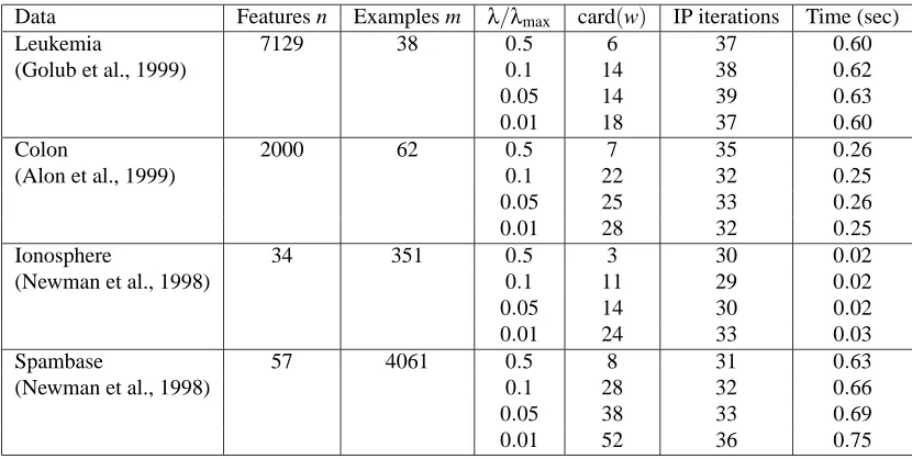
The data are four small or medium standard data sets taken from the UCI machine learning bench-mark repository (Newman et al., 1998) and other sources. The first data set is leukemia cancer gene expression data (Golub et al., 1999), the second is colon tumor gene expression data (Alon et al., 1999), the third is ionosphere data (Newman et al., 1998), and the fourth is spambase data (Newman et al., 1998).
For each data set, we considered four values of the regularization parameter: λ=0.5λmax,
λ=0.1λmax, λ=0.05λmax, and λ=0.01λmax. We discarded examples with missing data, and standardized each data set. The dimensions of each problem, along with the number of interior-point method iterations (IP iterations) needed, and the execution time, are given in Table 1. In reporting card(w), we consider a component wito be zero when
(1/m) AT(1−plog(v,w))
i
Data Features n Examples m λ/λmax card(w) IP iterations Time (sec)
Leukemia 7129 38 0.5 6 37 0.60
(Golub et al., 1999) 0.1 14 38 0.62
0.05 14 39 0.63
0.01 18 37 0.60
Colon 2000 62 0.5 7 35 0.26
(Alon et al., 1999) 0.1 22 32 0.25
0.05 25 33 0.26
0.01 28 32 0.25
Ionosphere 34 351 0.5 3 30 0.02
(Newman et al., 1998) 0.1 11 29 0.02
0.05 14 30 0.02
0.01 24 33 0.03
Spambase 57 4061 0.5 8 31 0.63
(Newman et al., 1998) 0.1 28 32 0.66
0.05 38 33 0.69
0.01 52 36 0.75
Table 1: Performance of the interior-point method on 4 data sets, each for 4 values ofλ.
whereτ=0.9999. This rule is inspired by the optimality condition in (8).
In all sixteen examples, around 35 iterations were required. We have observed this behavior over a large number of other examples as well. The execution times are well predicted by the complexity order min(m,n)2max(m,n).
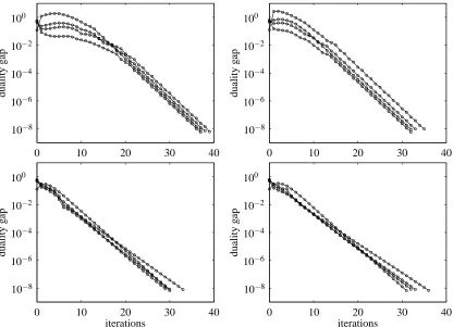
Figure 1 shows the progress of the interior-point method on the four data sets, for the same four values ofλ. The vertical axis shows duality gap, and the horizontal axis shows iteration number, which is the natural measure of computational effort when dense linear algebra methods are used. The figures show that the algorithm has linear convergence, with duality gap decreasing by a factor around 1.85 in each iteration.
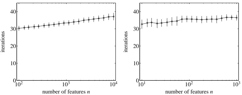
4.2 Randomly Generated Problems
To examine the effect of problem size on the number of iterations required, we generate 100 random problem instances for each of 20 values of n, ranging from n=100 to n=10000, with m=0.1n, that is, 10 times more features than examples. Each problem has an equal number of positive and negative examples, that is, m+ =m− =m/2. Features of positive (negative) examples are independent and identically distributed, drawn from a normal distribution
N
(v,1), where v is in turn drawn from a uniform distribution on[0,1]([−1,0]).For each of the 2000 data sets, we solve the`1-regularized LRP forλ=0.5λmax,λ=0.1λmax,
andλ=0.05λmax. The lefthand plot in Figure 2 shows the mean and standard deviation of the number of iterations required to solve the 100 problem instances associated with each value of n andλ. It can be seen that the number of iterations required is very near 35, for all 6000 problem instances.
ANINTERIOR-POINTMETHOD FORLARGE-SCALE`1-REGULARIZEDLOGISTICREGRESSION PSfrag replacements
duality
g
ap
0 10 20 30 40
50 10−10
10−8 10−6 10−4 10−2 100
PSfrag replacements
duality gap
0 10 20 30 40
50 10−10
10−8 10−6 10−4 10−2 100 duality g ap duality gap 0 10 20 30 40 50 10−10 10−8 10−6 10−4 10−2 100 duality gap iterations duality g ap
0 10 20 30 40
50 10−10
10−8 10−6 10−4 10−2 100 0 10 20 30 40 50 10−10 10−8 10−6 10−4 10−2 100 duality gap
iterations duality gap
0 10 20 30 40
50 10−10
10−8 10−6 10−4 10−2 100
iterations
duality
g
ap
Figure 1: Progress of the interior-point method on 4 data sets, showing duality gap versus iteration number. Top left: Leukemia cancer gene data set. Top right: Colon tumor gene data set.
Bottom left: Ionosphere data set. Bottom right: Spambase data set.
of the number of iterations required to solve the 100 problem instances associated with each value of n andλ. The results are quite similar to the case with m=0.1n.
5. Truncated Newton Interior-Point Method
In this section we describe a variation on our interior-point method that can handle very large prob-lems, provided the data matrix A is sparse, at the cost of having a run time that is less predictable. The basic idea is to compute the search direction approximately, using a preconditioned conjugate gradients (PCG) method. When the search direction in Newton’s method is computed approxi-mately, using an iterative method such as PCG, the overall algorithm is called a conjugate gradient
Newton method, or a truncated Newton method (Ruszczynski, 2006; Dembo and Steihaug, 1983).
Truncated Newton methods have been applied to interior-point methods (see, for example, Vanden-berghe and Boyd, 1995 and Portugal et al., 2000).
5.1 Preconditioned Conjugate Gradients
The PCG algorithm (Demmel, 1997, §6.6) computes an approximate solution of the linear equations
KOH, KIM ANDBOYD
PSfrag replacements
number of features n
iterations
102 103 104
0 10 20 30 40
102 103 104
0 10 20 30 40
number of features n
iterations
101 102 103
10 20 30 40
Figure 2: Average number of iterations required to solve 100 randomly generated `1-regularized LRPs with different problem size and regularization parameter. Left: n=10m. Right:
n=0.1m. Error bars show standard deviation.
PRECONDITIONED CONJUGATE GRADIENTS ALGORITHM
given relative toleranceεpcg>0, iteration limit Npcg, and x0∈Rk k :=0, r0:=Hx0−g, p1:=−P−1g, y0:=P−1r0.
repeat
k :=k+1
z :=H pk
θk:=yTk−1rk−1/pTkz
xk:=xk−1+θkpk
rk:=rk−1−θkz
yk:=P−1rk
µk+1:=yTkrk/yTk−1rk−1 pk+1:=yk+µk+1pk
until krkk2/kgk2≤εpcgor k=Npcg.
Each iteration of the PCG algorithm involves a handful of inner products, the matrix-vector product H pk and a solve step with P in computing P−1rk. With exact arithmetic, and ignoring the
stopping condition, the PCG algorithm is guaranteed to compute the exact solution x=−H−1g in N steps. When P−1/2HP−1/2 is well conditioned, or has just a few extreme eigenvalues, the PCG algorithm can compute an approximate solution in a number of steps that can be far smaller than N. Since P−1rkis computed in each step, we need this computation to be efficient.
5.2 Truncated Newton Interior-Point Method
We can compute H pkin the PCG algorithm using
H pk =
tbTD0b tbTD0A 0 tATD0b tATD0A+D1 D2
0 D2 D1
pk1 pk2 pk3 =
bTu ATu+D1pk2
D2pk2+D1pk3
,
where u=tD0(bpk1+Apk2)∈Rm. The cost of computing H pk is O(p) flops when A is sparse
with p nonzero elements. (We assume p≥n, which holds if each example has at least one nonzero
feature.)
We now describe a simple choice for the preconditioner P. The Hessian can be written as
H=t∇2lavg(v,w) +∇2Φ(w,u).
To obtain the preconditioner, we replace the first term with its diagonal part, to get
P=diag t∇2lavg(v,w)
+∇2Φ(w,u) =
d0 0 0
0 D3 D2
0 D2 D1
, (17)
where
d0=tbTD0b, D3=diag(tATD0A) +D1.
(Here diag(S) is the diagonal matrix obtained by setting the off-diagonal entries of the matrix S to zero.) This preconditioner approximates the Hessian of tlavg with its diagonal entries, while
retaining the Hessian of the logarithmic barrier. For this preconditioner, P−1rk can be computed
cheaply as
P−1rk =
d0 0 0
0 D3 D2
0 D2 D1
−1
rk1 rk2 rk3 =
rk1/d0
(D1D3−D22)−1(D1rk2−D2rk3) (D1D3−D22)−1(−D2rk2+D3rk3)
,
which requires O(n)flops.
We can now explain how implicit standardization can be carried out. When using standardized data, we work with the matrix Astd defined in (20), instead of A. As mentioned in Appendix A,
Astd is in general dense, so we should not form the matrix. In the truncated Newton interior-point method we do not need to form the matrix Astd; we only need a method for multiplying a vector by
Astd and a method for multiplying a vector by Astd T. But this is easily done efficiently, using the
fact that Astdis a sparse matrix (i.e., A) times a diagonal matrix, plus a rank-one matrix; see (20) in Appendix A.
There are several good choices for the initial point in the PCG algorithm (labeled x0 in
The PCG relative tolerance parameterεpcghas to be carefully chosen to obtain good efficiency in a truncated Newton method. If the tolerance is too small, too many PCG steps are needed to compute each search direction; if the tolerance is too high, then the computed search directions do not give adequate reduction in duality gap per iteration. We experimented with several methods of adjusting the PCG relative tolerance, and found good results with the adaptive rule
εpcg=min{0.1,ξη/kgk2}, (18)
where g is the gradient and η is the duality gap at the current iterate. Here, ξ is an algorithm parameter. We have found thatξ=0.3 works well for a wide range of problems. In other words, we solve the Newton system with low accuracy (but never worse than 10%) at early iterations, and solve it more accurately as the duality gap decreases. This adaptive rule is similar in spirit to standard methods used in inexact and truncated Newton methods (see Nocedal and Wright, 1999).
The computational effort of the truncated Newton interior-point algorithm is the product of
s, the total number of PCG steps required over all iterations, and the cost of a PCG step, which
is O(p), where p is the number of nonzero entries in A, that is, the total number of (nonzero) features appearing in all examples. In extensive testing, we found the truncated Newton interior-point method to be very efficient, requiring a total number of PCG steps ranging between a few hundred (for medium size problems) and several thousand (for large problems). For medium size (and sparse) problems it was faster than the basic interior-point method; moreover the truncated Newton interior-point method was able to solve very large problems, for which forming the Hessian
H (let alone computing the search direction) would be prohibitively expensive.
While the total number of iterations in the basic interior-point method is around 35, and nearly independent of the problem size and problem data, the total number of PCG iterations required by the truncated Newton interior-point method can vary significantly with problem data and the value of the regularization parameterλ. In particular, for small values ofλ(which lead to large values of card(w)), the truncated Newton interior-point method requires a larger total number of PCG steps. Algorithm performance that depends substantially on problem data, as well as problem dimension, is typical of all iterative (i.e., non direct) methods, and is the price paid for the ability to solve very large problems.
5.3 Numerical Examples
In this section we give some numerical examples to illustrate the performance of the truncated Newton interior-point method. We use the same algorithm parameters for line search, update rule, and stopping criterion as those used in Section 4, and the PCG tolerance given in (18) with ξ=
0.3. We chose the parameter Npcg to be large enough (5000) that the iteration limit was never
reached in our experiments; the typical number of PCG iterations was far smaller. The algorithm is implemented in both Matlab and C, on a 3.2GHz Pentium IV running Linux, except for very large problems. For very large problems whose data could not be handled on this computer, the method was run on AMD Opteron 254 with 8GB main memory. The C implementation is available online atwww.stanford.edu/˜boyd/l1_logreg.
5.3.1 A MEDIUMSPARSEPROBLEM
ANINTERIOR-POINTMETHOD FORLARGE-SCALE`1-REGULARIZEDLOGISTICREGRESSION PSfrag replacements
iterations
duality
g
ap
0 10 20 30 40
50 10−10
10−8 10−6 10−4 10−2 100
(a),(b),(c) (d)
0 10 20 30 40 50 10−10 10−8 10−6 10−4 10−2 100 (a),(b),(c)
(d)
cumulative PCG iterations
duality
g
ap
0 200 400 600 700 1000 10−10
10−8 10−6 10−4 10−2 100
(a) (b) (c) (d)
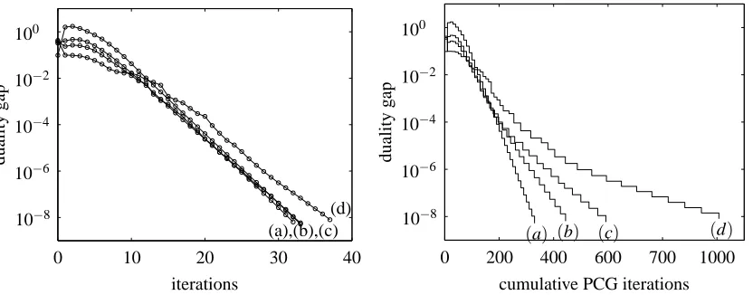
Figure 3: Progress of the truncated Newton interior-point method on the Internet advertisements data set with four regularization parameters: (a)λ=0.5λmax, (b)λ=0.1λmax, (c)λ=
0.05λmax, and (d)λ=0.01λmax.
matrix A is p=39011. We standardized the data set using implicit standardization, as explained in Section 5.2, solving four`1-regularized LRPs, with λ=0.5λmax, λ=0.1λmax, λ=0.05λmax,
andλ=0.01λmax. Figure 3 shows the convergence behavior. The lefthand plot shows the duality gap versus outer iterations; the righthand plot shows duality gap versus cumulative PCG iterations, which is the more accurate measure of computational effort.
The lefthand plot shows that the number of Newton iterations required to solve the problem is not much more than in the basic interior-point method described in Section 3. The righthand plot shows that the total number of PCG steps is several hundred, and depends substantially on the value ofλ. Thus, the search directions are computed using on the order of ten PCG iterations.
To give a very rough comparison with the direct method applied to this sparse problem, the truncated Newton interior-point method is much more efficient than the basic interior-point method that does not exploit the sparsity of the data. It is comparable to or faster than the basic interior-point method that uses sparse linear algebra methods, when the regularization parameter is not too small.
5.3.2 A LARGESPARSEPROBLEM
Our next example uses the 20 Newsgroups data set (Lang, 1995). We processed the data set in a way similar to Keerthi and DeCoste (2005). The positive class consists of the 10 groups with names of form sci.*, comp.*, and misc.forsale, and the negative class consists of the other 10 groups. We used McCallum’s Rainbow program (McCallum, 1996) with the command
rainbow -g 3 -h -s -O 2 -i
to tokenize the (text) data set. These options specify trigrams, skip message headers, no stoplist, and drop terms occurring fewer than two times. The resulting data set has n=777811 features (trigrams) and m=11314 examples (articles). Each example contains an average of 425 nonzero features. The total number of nonzero entries in the data matrix A is p=4802169. We standardized the data set using implicit standardization, as explained in Section 5.2, solving three`1-regularized
KOH, KIM ANDBOYD
λ/λmax card(w) Iterations PCG iterations Time (sec)
0.5 9 43 558 134
0.1 544 60 1036 256
0.05 2531 58 2090 501
Table 2: Performance of truncated Newton interior-point method on the 20 newsgroup data set (n=777811 features, m=11314 examples) for 3 values ofλ.
PSfrag replacements
iterations
duality
g
ap
0 20 40 60
80 100 10−10
10−8 10−6 10−4 10−2 100
(a) (c()b)
0 20 40 60 80 100 10−10 10−8 10−6 10−4 10−2 100
(a) (b) (c)
cumulative PCG iterations
duality
g
ap
0 500 1000 1500 2000 10−10
10−8 10−6 10−4 10−2 100
(a) (b) (c)
Figure 4: Progress of the truncated Newton interior-point method on the 20 Newsgroups data set for (a)λ=0.5λmax, (b) λ=0.1λmax, and (c) λ=0.05λmax. Left. Duality gap versus iterations. Right. Duality gap versus cumulative PCG iterations.
the cardinality of the optimal solution is around 10000 and comparable to the number of examples.) The performance of the algorithm, and the cardinality of the weight vectors, is given in Table 2. Figure 4 shows the progress of the algorithm, with duality gap versus iteration (lefthand plot), and duality gap versus cumulative PCG iteration (righthand plot).
The number of iterations required to solve the problems ranges between 43 and 60, depending on
λ. The more relevant measure of computational effort is the total number of PCG iterations, which ranges between around 500 and 2000, again, increasing with decreasingλ, which corresponds to increasing card(w). The average number of PCG iterations, per iteration of the truncated Newton interior-point method, is around 13 forλ=0.5λmax, 17 forλ=0.1λmax, and 36 forλ=0.05λmax. (The variance in the number of PCG iterations required per iteration, however, is large.) The running time is consistent with a cost of around 0.24 seconds per PCG iteration. The increase in running time, for decreasing λ, is due primarily to an increase in the average number of PCG iterations required per iteration, but also from an increase in the overall number of iterations required.
5.3.3 RANDOMLYGENERATEDPROBLEMS
number of features n
runtime
in
seconds
102 103 104 105 106 107 10−2
10−1 100 101 102 103 104
λ=0.5λmax
λ=0.1λmax λ=0.05λmax
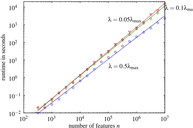
Figure 5: Runtime of the truncated Newton interior-point method, for randomly generated sparse problems, with three values ofλ.
set using implicit standardization, as explained in Section 5.2, solving each problem instance for the three values λ=0.5λmax, λ=0.1λmax, and λ=0.05λmax. The total runtime, for the 63 `1
-regularized LRPs, is shown in Figure 5. The plot shows that runtime increases asλdecreases, and grows approximately linearly with problem size.
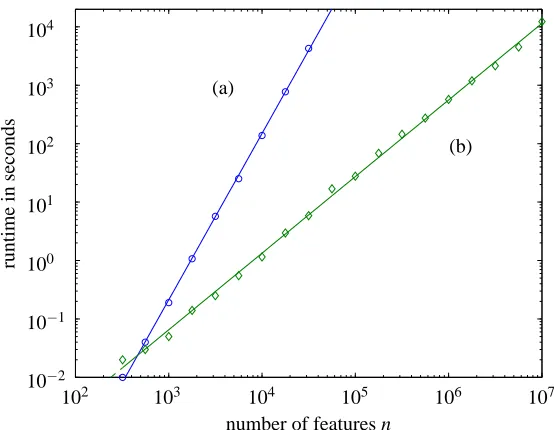
We compare the runtimes of the truncated Newton interior-point and the basic interior-point method using dense linear algebra methods to compute the search direction. Figure 6 shows the re-sults forλ=0.1λmax. The truncated Newton interior-point method is far more efficient for medium problems. For large problems, the basic interior-point method fails due to memory limitations, or extremely long computation times.
By fitting an exponent to the data over the range from n=320 to the largest problem successfully solved by each method, we find that the basic interior-point method scales as O(n2.8) (which is consistent with the basic flop count analysis, which predicts O(n3)). For the truncated Newton interior-point method, the empirical complexity is O(n1.3).
When sparse matrix methods are used to compute the search direction in the basic interior-point method, we get an empirical complexity of O(n2.2) for the Matlab implementation of the basic interior-point method that uses sparse matrix methods, showing a good efficiency gain over dense methods, for medium scale problems. The C implementation would have the same empirical complexity as the Matlab one with a smaller constant hidden in the O(·)notation.
5.3.4 PRECONDITIONERPERFORMANCE
number of features n
runtime
in
seconds
102 103 104 105 106 107 10−2
10−1 100 101 102 103 104
(a)
(b)
Figure 6: Runtime of (a) the basic interior-point method and (b) the truncated Newton interior-point method, for a family of randomly generated sparse problems.
PSfrag replacements
index
eigen
v
alues
preconditioned Hessian Hessian
1 1000 2000 3000 4000 10−1
100 101 102 103 104
105
index eigenvalues
preconditioned Hessian Hessian
1 1000 2000 3000 4000 10−1 100 101 102 103 104 105
index
eigen
v
alues preconditioned Hessian Hessian
1 1000 2000 3000 4000 10−2
100 102 104 106 108
1010
Figure 7: Eigenvalue distributions of Hessian and preconditionned Hessian, at the 15th iterate, for the colon gene tumor problem, forλ=0.5λmax(left) andλ=0.05λmax(right).
with just a few extreme eigenvalues, which explains the good performance with relatively few PCG iterations per iteration (Demmel, 1997, §6.6).
6. Computing the Regularization Path
In this section we consider the problem of solving the `1-regularized LRP for M values of the
regularization parameterλ,
λmax=λ1>λ2>· · ·>λM>0.
is efficient when multiple processors are used, since the LRPs can be solved simultaneously, on different processors. But when one processor is used, we can solve these M problems much more efficiently by solving them sequentially, using the previously computed solution as a starting point for the next computation. This is called a warm-start approach.
We first note that the solution forλ=λ1=λmaxis(log(m+/m−),0,0). Since this point does not satisfy|wi|<ui, it cannot be used to initialize the computation forλ=λ2. We modify it by adding
a small increment to u to get
(v(1),w(1),u(1)) = (log(m+/m−),0,(εabs/(nλ))1),
which is strictly feasible. In fact, it is on the central path with parameter t =2n/εabs, and so is
εabs-suboptimal. Note that so far we have expended no computational effort.
Now for k=2, . . . ,M we compute the solution(v(k),w(k),u(k))of the problem withλ=λk, by
applying the interior-point method, with starting point modified to be
(vinit,winit,uinit) = (v(k−1),w(k−1),u(k−1)),
and initial value of t set to t=2n/εabs.
In the warm-start technique described above, the number of grid points, M, is fixed in advance. The grid points (and M) can be chosen adaptively on the fly, while taking into account the curvature of the regularization path trajectories, as described in Park and Hastie (2006a).
6.1 Numerical Results
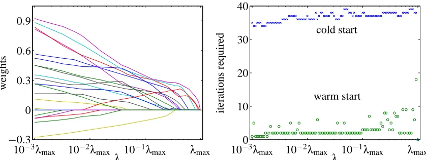
Our first example is the leukemia cancer gene expression data, for M=100 values ofλ, uniformly distributed on a logarithmic scale over the interval [0.001λmax,λmax]. (For this example, λmax=
0.37.) The left plot in Figure 8 shows the regularization path, that is, w(k), versus regularization parameterλ. The right plot shows the number of iterations required to solve each problem from a warm-start, and from a cold-start.
The number of cold-start iterations required is always near 36, while the number of warm-start iterations varies, but is always smaller, and typically much smaller, with an average value of 3.1. Thus the computational savings for this example is over 11 : 1.
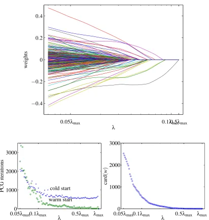
Our second example is the 20 Newsgroups data set, with M=100 values ofλuniformly spaced on a logarithmic scale over[0.05λmax,λmax]. For this problem we haveλmax=0.12. The top plot in Figure 9 shows the regularization path. The bottom left plot shows the total number of PCG iterations required to solve each problem, with the warm-start and cold-start methods. The bottom right plot shows the cardinality of w as a function ofλ.
Here too the warm-start method gives a substantial advantage over the cold-start method, at least forλnot too small, that is, as long as the optimal weight vector is relatively sparse. The total runtime using the warm-start method is around 2.8 hours, and the total runtime using the cold-start method is around 6.2 hours, so the warm-start methods gives a savings of around 2 : 1. If we consider only the range from 0.1λmaxtoλmax, the savings increases to 5 : 1.