Infinite-
σ
Limits For Tikhonov Regularization
Ross A. Lippert [email protected]
Department of Mathematics
Massachusetts Institute of Technology 77 Massachusetts Avenue
Cambridge, MA 02139-4307, USA
Ryan M. Rifkin [email protected]
Honda Research Institute USA, Inc. 145 Tremont Street
Boston, MA 02111, USA
Editor: Gabor Lugosi
Abstract
We consider the problem of Tikhonov regularization with a general convex loss function: this for-malism includes support vector machines and regularized least squares. For a family of kernels that includes the Gaussian, parameterized by a “bandwidth” parameterσ, we characterize the limiting solution asσ→∞.In particular, we show that if we set the regularization parameterλ=˜λσ−2p, the regularization term of the Tikhonov problem tends to an indicator function on polynomials of degree⌊p⌋(with residual regularization in the case where p∈Z). The proof rests on two key ideas:
epi-convergence, a notion of functional convergence under which limits of minimizers converge to
minimizers of limits, and a value-based formulation of learning, where we work with regularization on the function output values (y) as opposed to the function expansion coefficients in the RKHS. Our result generalizes and unifies previous results in this area.
Keywords: Tikhonov regularization, Gaussian kernel, theory, kernel machines
1. Introduction
Given a data set(x1,yˆ1), . . . ,(xn,yˆn)∈Rd×R, the supervised learning task is to construct a function f(x) that, given a new point, x, will predict the associated y value. A number of methods for this problem have been studied. One popular family of techniques is Tikhonov regularization in a Reproducing Kernel Hilbert Space (RKHS) (Evgeniou et al., 2000):
inf
f∈H
(
nλ||f||2κ+
n
∑
i=1
v(f(xi),yˆi)
)
.
Here, v :R×R→Ris a loss function indicating the price we pay when we see xi, predict f(xi),
and the true value is ˆyi. The squared norm, ||f||2κ, in the RKHS
H
involves the kernel function κ(Aronszajn, 1950). The regularization constant,λ>0, controls the trade-off between fitting the training set accurately (minimizing the penalties) and forcing f to be smooth inH
. The Representerthe Tikhonov regularization can be written in the form
f(x) =
n
∑
i=1
ciκ(xi,x).
In practice, solving a Tikhonov regularization problem is equivalent to finding the expansion coef-ficients ci.
One popular choice forκis the Gaussian kernelκσ(x,x′) =e−||
x−x′||2
2σ2 , whereσis the bandwidth
of the Gaussian. Common choices for v include the square loss, v(y,yˆ) = (y−yˆ)2, and the hinge
loss, v(y,yˆ) =max{0,1−y ˆy}, which lead to regularized least squares and support vector machines, respectively.
Our work was originally motivated by the empirical observation that on a range of tasks, reg-ularized least squares achieved very good performance with very largeσ. (For example, we could often choose σ so large that every kernel product between pairs of training points was between
.99999 and 1.) To get good results with largeσ, it was necessary to makeλsmall. We decided to study this relationship.
Regularized least squares (RLS) is an especially simple Tikhonov regularization algorithm: “training” RLS simply involves solving a system of linear equations. In particular, defining the matrix K via Ki j =κ(xi,xj), the RLS expansion coefficients c are given by (K+nλI)c=y, orˆ c= (K+nλI)−1y. Given a test point xˆ
0, we define the n-vector k via ki=κ(x0,xi), and we have, for
RLS with a fixed bandwidth,
f(x0) =kt(K+nλI)−1yˆ.
In Lippert and Rifkin (2006), we studied the limit of this expression as σ→∞, showing that if we set λ=˜λσ−2p−1 for p a positive integer, the infinite-σ limit converges (pointwise) to the
degree p polynomial with minimal empirical risk on the training set. The asymptotic predictions are equivalent to those we would get if we simply fit an (unregularized) degree p polynomial to our training data.
In Keerthi and Lin (2003), a similar phenomenon was also noticed for support vector machines (SVM) with Gaussian kernels, where it was observed that the SVM function could be made to converge (in the infinite-σlimit) to a linear function which minimized the hinge loss plus a residual regularization (discussed further below). In that work, only a linear result was obtained; no results were given for general polynomial approximation limits.
In the current work, we unify and generalize these results, showing that the occurrence of these polynomial approximation limits is a general phenomenon, which holds across all convex loss func-tions and a wide variety of kernels taking the formκσ(x,x′) =κ(x/σ,x′/σ). Our main result is that for a convex loss function and a valid kernel, if we takeσ→∞andλ=˜λσ−2p, the regularization
term of the Tikhonov problem tends to an indicator function on polynomials of degree ⌊p⌋. In the case where p∈Z, there is residual regularization on the degree-p coefficients of the limiting polynomial.
Our proof relies on two key ideas. The first is the notion of epi-convergence, a functional convergence under which limits of minimizers converge to minimizers of limits. This notion allows us to characterize the limiting Tikhonov regularization problem in a mathematically precise way. The second notion is a value-based formulation of learning. The idea is that instead of working with the expansion coefficients in the RKHS (ci), we can write the regularization problem directly
in terms of the predicted values (yi). This allows us to avoid combining and canceling terms whose
2. Notation
In this section, we describe the notation we use throughout the paper. Some of our choices are non-standard, and we try to indicate these.
2.1 Data Sets and Regularization
We refer to a general d dimensional vector with the symbol x (plus superscripts or subscripts). We assume a fixed set of n training points xi ∈Rd (1≤i≤n) and refer to the totality of these data
points by X , such that for any f :Rd →R, f(X) = (f(x1) ··· f(xn) )t is the vector of values
over the points and for any g :Rd×Rd→R, g(X,X)is the matrix of values over pairs of points, i.e. [g(X,X)]i j=g(xi,xj). We let x0represent an arbitrary “test point” not in the training set. We assume
we are given “true” ˆy values at the training points: ˆyi ∈R,1≤i≤n.While it is more common to
use ˆy to refer to the “predicted” output values and y to refer to the “true” output values, we find
this choice much more notationally convenient, because our value-based formulation of learning (3) requires us to work with the predicted values very frequently.
Tikhonov regularization is given by
inf
f∈H
(
nλ||f||2κ+
n
∑
i=1
v(f(xi),yˆi)
)
. (1)
Tikhonov regularization can be used for both classification and regression tasks, but we refer to the function f as the regularized solution in all cases. We call the left-hand portion the regularization
term, and the right-hand portion the loss term. We assume a loss function v(y,yˆ)that is convex in its first argument and minimized at y=y (thereby ruling out, for example, the 0/1 “misclassificationˆ rate”). We call such a loss function valid. Aside from convexity, we will be unconcerned with the form of the loss function and often take the loss term in the optimization in (1) to be some convex function V :Rn→Rwhich is minimized by the vector ˆy of ˆyi’s.
To avoid confusion, when subscripting over d dimensional indices, we use letters from the beginning of the alphabet (a,b,c, . . .), while using letters from the middle (i,j, . . .) for n dimensional indices.
When referring to optimization problems, we use an over-dot (e.g. ˙y) to denote optimizing
quantities. We are not time-differentiating anything in this work, so this should not cause confusion.
2.2 Polynomials
By a multi-index we refer to I∈Zd such that Ia≥0. Given x∈Rd we write xI =∏da=1xIaa. We
also write XI to denote(xI1 ··· xnI)t. The degree of a multi-index is|I|=∑d
a=1Ia. We use the
“choose” notation
|I| I
= |I|!
∏d a=1Ia!
.
Let {Ii}∞i=0 be an ordering of multi-indices which is non-decreasing by degree (in particular, I0= (0 ··· 0)). We consider this fixed for the remainder of the work. Define dc=|{I :|I| ≤c}|
and note that dc=
d+c+1
c
. Put differently,{I :|I|=c}={Ii: dc−1≤i<dc}.
Given a data set, while the monomials xIi are linearly independent as functions, no more than
linearly independent. This is equivalent to requiring that the data not reside on the zero-set of a low degree system polynomials. This is not an unreasonable assumption for data which is presumed to have been generated by distributions supported onRnor some sphere inRn. Throughout this paper, we assume that our data is generic. It is possible to carry out the subsequent derivations without it, but the modifications which result are tedious. In particular, parts of Theorem 12, which treat the first n monomials XIi as linearly independent (e.g. assuming v
α(X) is non-singular in the proof), would need to be replaced with analogous statements about the first n monomials XIi j which are
linearly independent, and various power-series expansion coefficients would have to be adjusted accordingly. Additionally, our main result requires not only genericity of the data, but also that
n>dpwhere p is the degree of the asymptotic regularized solution.
2.3 Kernels
It is convenient to use infinite matrices and vectors to express certain infinite series. Where used, the convergence of the underlying series implies the convergence of any infinite sums that arise from the matrix products we form, and we will not attempt to define any inverses of non-diagonal infinite matrices. This is merely a notational device to avoid excessive explicit indexing and summing in the formulas ahead. Additionally, since many of our vectors come from power series expansions, we adopt the convention of indexing such vectors and matrices starting from 0.
A Reproducing Kernel Hilbert Space (RKHS) is characterized by a kernel functionκ. Ifκhas a power series expansion, we may write
κ(x,x′) =
∑
i,j≥0
Mi jxIix′Ij
= v(x)Mv(x′)t
where M∈R∞×∞is an infinite matrix and v(x) = (1 xI1 xI2 ···)∈R1×∞ is an infinite row-vector valued function of x. We emphasize that M is an infinite matrix induced by the kernel function
κand the ordering of multi-indices; it has nothing to do with our data set.
We say that a kernel is valid if every finite upper-left submatrix of M is symmetric and positive definite; in this case, we also say that the infinite matrix M is symmetric positive definite. This con-dition is the one we use in our main proof; however, it can be difficult to check. It is independent of the Mercer property (which states that the kernel matrixκ(X,X)for a set X is positive semidefinite), sinceκ(x,x′) = 1−1xx′ is valid but not Mercer, and exp(−(x3−x′3)2)is Mercer but not valid. This
notion is, basically, that the feature space ofκcan approximate any polynomial function near the origin to arbitrary accuracy. We are not aware of any mention of this property in the literature. The following lemma gives a stronger condition that implies validity.
Lemma 1 Ifκ(x,x′) =∑c≥0(x·x′)cgc(x)gc(x′)for some analytic functions gc(x)such that gc(0)6=0, thenκis a valid kernel.
Proof By the multinomial theorem,
(x·x′)c=
d
∑
i=1 xix′i
!c
=
∑
|I|=c
|I| I
Let gc(x) =∑IGcIxI, and note gc(0) =Gc0, thus
κ(x,x′) =
∑
I,J,c≥0|E
∑
|=c
|E| E
xI+EGcIGcJx′J+E
=
∑
I,J,E
|Ik| Ik
xI+EG|E|IG|E|Jx′J+E
=
∑
I,J≥E
xIG|E|(I−E)
|E| E
G|E|(J−E)x′J
= v(x)LLtv(x′)
where Li j =
|Ij| Ij
12
G|Ij|(Ii−Ij)when Ii≥Ij and 0 otherwise. In other words, L is an infinite lower
triangular matrix with non-vanishing diagonal elements (since Gc06=0 for all c).
Since M=LLt, the upper-left submatrices of L are the Cholesky factors of the corresponding upper-left submatrix of M, and thus M is positive definite.
We note thatκ(x,x′) =exp(−12||x−x′||2)can be written in the form of Lemma 1:
κ(x,x′) = exp
−12||x||2
exp(x·x′)exp
−12||x′||2
=
∞
∑
c=0
(x·x′)c c! exp
−12||x||2
exp
−12||x′||2
=
∞
∑
c=0
(x·x′)cgc(x)gc(x′),
where gc(x) =√1c!exp(−12||x||2).
We will consider kernel functionsκσ which are parametrized by a bandwidth parameterσ(or
s= 1
σ). We will occasionally use Kσto refer to the matrix whose i,jth entryκσ(xi,xj), for 1≤i≤ n,1≤ j≤n. We will also use kσ to denote the n-vector whose ith entry isκσ(xi,x0)— the kernel product between the ith training point xiand the test point x0.
3. Value-Based Learning Formulation
In this section, we discuss our value-based learning formulation. Using the representer theorem and basic facts about RKHS, the standard Tikhonov regularization problem (1) can be written in terms of the expansion coefficients c and the kernel matrix K:
inf
c∈Rn
(
nλctKc+
∑
n i=1v([Kc]i,yˆi)
)
. (2)
The predicted values on the training set are y= f(X) =Kc. If the kernel matrix K is invertible
(which is the case for a Gaussian kernel and a generic data set), then c=K−1y, and we can rewrite
the minimization as
inf
y∈Rn
where V is convex (V(y) =∑n
i=1vi(yi,yˆi)).
While problem 2 is explicit in the coefficients of the expansion of the regularized solution, problem 3 is explicit in the predicted values yi. The purpose behind our choice of formulation is to
avoid the unnecessary complexities which result from replacingκwithκσand taking limits as both
ci andκσ(x,xi) change separately withσ: note that in problem 3, only the regularization term is varying withσ.
In this section, we will show how our formulation achieves this, by allowing us to state a sin-gle optimization problem which simultaneously solves the Tikhonov regularization problem on the training data and evaluates the resulting function on the test data.
Theorem 2 Let y=
y0 y1
∈Rm+nbe a block vector with y0∈Rm,y1∈Rnand K=
K00 K01 K10 K11
∈
R(m+n)×(m+n)be a positive definite matrix. For any V :Rn→R, if ˙y minimizes
ytK−1y+V(y1) (4) then ˙y1minimizes
yt1K11−1y1+V(y1) (5) and ˙y0=K01K11−1y˙1.
Proof
inf
y0,y1{y
tK−1y+V(y1) }=inf
y1{infy0{y tK−1y
}+V(y1)}. (6)
Let K−1=K¯ =
¯
K00 K01¯
¯
K10 K11¯
. Consider minimizing ytK−1y=yt0K00y0¯ +2yt0K01y1¯ +yt1K11y1¯ . For fixed y1, ˙y0=−K¯00−1K01y1¯ =K01K11−1y1by (17) of Lemma 15. Thus,
inf
y0
ytK−1y =yt1(K11¯ −K10¯ K¯00−1K01¯ )y1=yt1K11−1y1
by (19) of Lemma 15.
We contextualize this result in terms of the Tikhonov learning problem with the following corol-lary.
Corollary 3 Let X be a given set of data points x1, . . . ,xn with x0 a test point. Letκbe a valid kernel function and V :Rn→Rbe arbitrary. If ˙y= (y˙
0 y˙1 ··· y˙n)t is the minimizer of nλytκ
x0 X
,
x0 X
−1
y+V(y1, . . . ,yn)
then(y˙1 ··· y˙n)t minimizes nλytκ(X,X)−1y+V(y)and
˙
y0=∑ni=1ciκ(x0,xi), for c=κ(X,X)−1(y1˙ ··· y˙n)t.
Thus, when solving for y instead of c, we can evaluate the function at a test point x0by including
the additional point in a larger minimization problem where the test point contributes to the regular-ization, but not the loss. When taking limits, we are going to work directly with the yi, and we are
4. Epi-limits, Convex Functions, and Quadratic Forms
The relationship between the limit of a function and the limit of its minimizer(s) is subtle, and it is very easy to make incorrect statements. For convex functions there are substantial results on this subject, which we review; we essentially follow the development of Rockafellar and Wets (2004, chap. 7). Since the component of our objective which depends on the limiting parameter is a quadratic form, we will eventually specialize the results to quadratic forms.
Definition 4 (epigraphs) Given a function f :Rn→(−∞,∞], its epigraph, epi f is the subset of
R×Rngiven by
epi f ={(z,x): z≥ f(x)}.
We call f closed, convex, or proper if those statements are true of epi f (proper referring to epi f being neither /0norRn+1).
The functions we will be interested in are closed, convex, and proper. We will therefore adopt the abbreviation ccp for these conditions. Additionally, since we will be studying parameterized functions, fs, for 0<s as s→0, we say that such a family of functions is eventually convex (or
closed, or proper) when there exists some s0>0 such that fsis convex (or closed, or proper) for all
0<s<s0.
We review the definition of lim inf and lim sup for functions of a single variable. Given h : (0,∞)→ (−∞,∞], it is clear that the functions infs′∈(0,s){h(s′)} and sups′∈(0,s){h(s′)} are
non-increasing and non-decreasing functions of (non-increasing) s respectively.
Definition 5 For h :(0,∞)→(−∞,∞],
lim inf
s→0 h(s) = sups>0
inf
s′∈(0,s){h(s
′)}
lim sup
s→0
h(s) = inf
s>0
(
sup
s′∈(0,s){
h(s′)}
)
.
As defined, either of the limits may take the value∞. A useful alternate characterization, which is immediate from the definition, is lim infs→0h(s) =h0iff∀ε>0,∃s0,∀s∈(0,s0): h(s)≥h0−ε, and
lim sups→0h(s) =h0iff∀ε>0,∃s0,∀s∈(0,s0): h(s)≤h0+ε, where either inequality can be strict
if h0<∞.
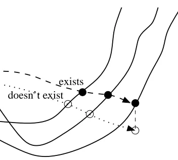
Definition 6 (epi-limits) We say lims→0fs=f if for all x0∈Rn, both the following properties hold:
Property 1:∀x :[0,∞)→Rncontinuous at x(0) =x0satisfies
lim inf
s→0 fs(x(s))≥ f(x0) (7)
Property 2:∃x :[0,∞)→Rncontinuous at x(0) =x0satisfying
lim sup
s→0
doesn’t exist exists
Figure 1: (property 1) of Definition 6 says that paths of points within epi fs cannot end up below
epi f , while (property 2) says that at least one such path hits every point of epi f .
This notion of functional limit is called an epigraphical limit (or epi-limit). Less formally, (property 1) is the condition that paths of the form (x(s),fs(x(s))) are, asymptotically, inside epi f , while
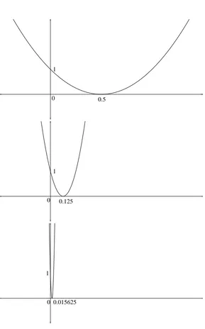
(property 2) asserts the existence of a path which hits the boundary of epi f , as depicted in figure 1. Considering (property 1) with the function x(s) =x0, it is clear that the epigraphical limit mi-norizes the pointwise limit (assuming both exist), but the two need not coincide. An example of this distinction is given by the family of functions
fs(x) =
2
sx(x−s) +1,
illustrated by Figure 2. The pointwise limit is f0(0) =1,f0(x) =∞for x6=0. The epi-limit is 0 at 0.
We say that a quadratic form is finite if f(x)<∞for all x. (We note in passing that if a quadratic form is not finite, f(x) =∞almost everywhere.) The pointwise and epi-limits of quadratic forms agree when the limiting quadratic form is finite, but the example in the figure is not of that sort. This behavior is typical of the applications we consider. In what follows, we take all functional limits to be epi-limits.
It is the epi-limit of functions which is appropriate for optimization theory, as the following theorem (a variation of one one from Rockafellar and Wets (2004)) shows.
Theorem 7 Let fs:Rn →(−∞,∞] be eventually ccp, with lims→0fs= f . If fs,f have unique minimizers ˙x(s),x then˙
lim
s→0x˙(s) =x˙ and lims→0fs(x˙(s)) =infx f(x).
Proof Givenδ>0, let Bδ={x∈Rn: f(x)< f(x˙) +2δ}. Since ˙x is the unique minimizer of f and f is ccp, Bδis bounded and open, and for any open neighborhood U of ˙x, ∃δ>0 : Bδ⊂U . Note
that x∈∂Bδiff f(x) = f(x˙) +2δ.
Let ˆx :[0,∞)→R satisfy property 2 of definition 6 with ˆx(0) =x. Let s0˙ >0 be such that
0.5 1
0
0.125 1
0
0 1
0.015625
Figure 2: The function above, fs(x) =2sx(x−s) +1, has different pointwise and epi-limits, having
By property 1 of definition 6, ∀x∈Rn,lim infs→0fs(x)≥ f(x), in particular,∀x∈∂Bδ, ∃s1∈
(0,s0),∀s∈ (0,s1): fs(x) ≥ f(x)−δ= f(x˙) +δ. Since ∂Bδ is compact, we can choose s1 ∈
(0,s0),∀x∈∂Bδ,s∈(0,s1): fs(x)≥ f(x˙) +δ.
Thus∀x∈∂Bδ,s<s1: fs(x)≥f(x˙) +δ>infx∈Bδ fs(x), and therefore ˙x(s)∈Bδby the convexity
of fs.
Summarizing, ∀δ>0,∃s1>0,∀s∈(0,s1): ˙x(s)∈Bδ. Hence ˙x(s)→x and we have the first˙
limit.
The second limit is a consequence of the first (lims→0x˙(s) =x) and definition 6. In particular,˙
lim sups→0fs(xˆ(s))≤ f(x˙)and f(x˙)≤lim infs→0fs(x˙(s)). Since∀s : fs(x˙(s))≤ fs(xˆ(s)), we have
lim sups→0fs(x˙(s))≤ f(x˙)and hence f(x˙)≤lim infs→0fs(x˙(s))≤lim sups→0fs(x˙(s))≤ f(x˙).
We now apply this theorem to characterize limits of quadratic forms (which are becoming infi-nite in the limit). The following lemma is elementary.
Lemma 8 Let A(s) be a continuous matrix-valued function. If A(0) is non-singular, then A(s)−1 exists for a neighborhood of s=0.
Lemma 9 Let Z(s)∈Rn×n be a continuous matrix valued function defined for s≥0 such that
Z(0) =0 and Z(s)is non-singular for s>0.
Let M(s) =
A(s) B(s)t B(s) C(s)
∈R(m+n)×(m+n)be a continuous symmetric matrix valued function
of s such that M(s)is positive semi-definite and C(s)is positive definite for s≥0. If
fs(x,y) =
x Z(s)−1y
t
A(s) B(s)t B(s) C(s)
x Z(s)−1y
then lims→0fs=f,where f(x,y) =
∞
y6=0
xt(A(0)−B(0)tC(0)−1B(0))x y=0 .
Proof Completing the square,
fs(x,y) =||x||A2˜(s)+||Z(s)−1y+C(s)−1B(s)x||2C(s)
where||v||W2 =vtW v and ˜A(s) =A(s)−B(s)tC(s)−1B(s). Note that ˜A(s) is positive semi-definite
and continuous at s=0.
Let b,c,s0>0 be chosen such that∀s<s0
b|| · ||>||B(s)· ||, || · ||C(s)>c|| · ||
(Such quantities arise from the the singular values of the matrices involved, which are continuous in s). Let z(s) =||Z(s)||(matrix 2-norm). Note: z is continuous with z(0) =0.
Let x(s),y(s)be continuous at s=0. If y(0)6=0, then for s<s0
p
fs(x(s),y(s)) ≥ ||Z(s)−1y(s) +C(s)−1B(s)x(s)||C(s)
by the triangle inequality
p
fs(x(s),y(s)) ≥ ||Z(s)−1y(s)||C(s)− ||B(s)x(s)||C(s)−1 > c||y(s)||
z(s) −
b c||x(s)||
= c
||y(s)||
z(s) −
b c2||x(s)||
.
By continuity,∃s1∈(0,s0)such that∀s∈(0,s1), ||x(s)||<3
2||x(0)||, ||y(s)||> 1
2||y(0)||,
b
c2||x(0)||<
||y(0)|| 6z(s) .
Thus, for all s<s1:pfs(x(s),y(s))>c||4zy((0s))||, and hence lim infs→0fs(x(s),y(s)) =∞, which
im-plies property 1 of definition 6 (and property 2, since lim inf≤lim sup). Otherwise (y(0) =0),
fs(x(s),y(s))≥ ||x(s)||2A˜(s)and thus
lim
s→0||x(s)|| 2
˜
A(s) ≤ lim infs→0 f(x(s),y(s))
||x(0)||2 ˜
A(0) ≤ lim infs→0 f(x(s),y(s))
(property 1). fs(x(s),y(s)) =||x(s)||A2˜(s) when y(s) =−Z(s)C(s)−
1B(s)x(s) (which is continuous
and vanishing at s=0), and thus
lim sup
s→0
f(x(s),y(s)) = lim
s→0||x(s)|| 2
˜
A(s)=||x(0)||
2 ˜ A(0)
(property 2).
The following application of the lemma allows us to deal with matrices which will be of specific interest to us.
Corollary 10 Let Z1(s)∈Rl×land Z2(s)∈Rn×nbe continuous matrix valued functions defined for s≥0 such that Zi(0) =0 and Zi(s)is non-singular for s>0.
Let M(s) =
A(s) B(s)t C(s)t B(s) D(s) E(s)t C(s) E(s) F(s)
∈R(l+m+n)×(l+m+n)be a continuous symmetric matrix
val-ued function of s such that M(s)is positive semi-definite and F(s)is positive definite for s≥0. If
fs(qa,qb,qc) =
Z1(s)qa qb Z2(s)−1qc
t
A(s) B(s)t C(s)t B(s) D(s) E(s)t C(s) E(s) F(s)
Z1(s)qa qb Z2(s)−1qc
then lims→0fs=f,where f(qa,qb,qc) =
∞
qc6=0 qtb(D(0)−E(0)tF(0)−1E(0))q
Proof We apply Lemma 9 to the quadratic form given by qa qb
Z2−1qc
t
Zt1AZ1 Zt1Bt BZ1 D
Z1tCt Et
(CZ1 E) F
qa qb
Z2−1qc
(s dependence suppressed).
We will have occasion to apply Corollary 10 when some of qa, qband qcare empty. In all cases,
the appropriate result can be re-derived under the convention that a quadratic form over a 0 variables is identically 0.1
5. Kernel Expansions and Regularization Limits
In this section, we present our key result, characterizing the asymptotic behavior of the regulariza-tion term of Tikhonov regularizaregulariza-tion. We define a family of quadratic forms on the polynomials in
x; these forms will turn out to be the limits of the quadratic Tikhonov regularizer.
Definition 11 Letκ(x,x′) =∑i,j≥0Mi jxIix′Ij, with M symmetric, positive definite. For any p>0, define RKp : f →[0,∞]by
Rκp(f) =
0 f(x) =∑0≤i≤d
⌊p⌋qix
Ii
∞ else , if p∈/Z
Rκp(f) =
qdp−1+1 .. . qdp
t C
qdp−1+1 .. . qdp
f(x) =∑0≤i≤dpqix
Ii
∞ else
, if p∈Z
where, for p∈Z, C= (Mbb−MbaMaa−1Mab)−1 where Maa and
Maa Mab Mba Mbb
are the dp−1×dp−1 and dp×dpupper-left submatrices of K.
The qi in the conditions for f above are arbitary, and hence the conditions are both equivalent to f ∈span{xI:|I| ≤p}. We have written the qiexplicitly merely to define the value Rκpwhen p∈Z.
Define v(X) = (1 XI1 XI2 ···)∈Rn×∞. Let v(X) = (vα(X) vβ(X) )be a block decompo-sition into an n×n block (a Vandermonde matrix on the data) and an n×∞block. Because our data set is generic, vα(X) is non-singular, and the interpolating polynomial through the points (xi,yi)
over the monomials{xIi: i<n}is given by f(x) =v
α(x)vα(X)−1y.
We now state and prove our key result, showing the convergence of the regularization term of Tikhonov regularization to Rκp.
Theorem 12 Let X be generic andκ(x,x′) =∑i,j≥0Mi jxIix′Ij be a valid kernel. Let p∈[0,|In−1|). Let fs(y) =s2pytκ(sX,sX)−1y. Then
lim
s→0fs= f,
where f(y) =Rκp(q), and q(x) =vα(x)q˜=∑0≤i<nq˜ixIi and ˜q=vα(X)−1y.
Proof Recalling that vα(X)is non-singular by genericity, defineχ=vα(X)−1v
β(X). LetΣ(s)be the infinite diagonal matrix valued function of s whose ithdiagonal element is s|Ii|. We define a block
decompositionΣ(s) =
Σ
α(s) 0 0 Σβ(s)
whereΣα(s)is n×n. We likewise partition M into blocks
M=
Mαα Mαβ Mβα Mββ
where Mααis n×n.
Thus,
κ(sX,sX)
= v(X)Σ(s)MΣ(s)v(X)t
= vα(X) (I χ)Σ(s)MΣ(s)
I χt
vα(X)t
= vα(X)Σα(s) (I Σα(s)−1χΣ
β(s) )M
I
(Σα(s)−1χΣ
β(s))t
Σα(s)vα(X)t
= vα(X)Σα(s) (I χ˜(s) )M
I
˜
χ(s)t
Σα(s)vα(X)t
= vα(X)Σα(s)M˜(s)Σα(s)vα(X)t,
where we have implicitly defined
˜
χ(s) ≡ Σα(s)−1χΣβ(s) ˜
M(s) ≡ (I χ˜(s) )M
I
˜
χ(s)t
.
For 0≤i<n, 0≤ j<∞, the i,jth entry of ˜χ(s) is s|Ij+n|−|Ii|χ
i j, and|Ij+n| − |Ii| ≥0. Thus,
lims→0χ˜(s)exists and we denote it ˜χ(0). We note that ˜χi j(0)is non-zero if and only if|Ii|=|Ij+n|.
In particular,
˜
χi j(0) =
χ
i j d|In|−1≤i<n and 0≤j<d|In|−n
0 otherwise
Therefore, lims→0M˜(s) = (I χ˜(0) )M
I
˜
χ(0)t
exists and is positive definite (since(I χ˜(0) )t
is full rank); we denote it by ˜M(0). Additionally, since the first d|In|−1 rows of ˜χ(0)(and therefore
the first d|In|−1columns of ˜χ(0)
t) are identically zero, the d
|In|−1×d|In|−1upper-left submatrices of
˜
M(0)and M are equal. Summarizing,
fs(y) = s2pytκ(sX,sX)−1y
= (vα(X)−1y)t(spΣα(1/s))M˜(s)−1(spΣ
α(1/s))(vα(X)−1y) = q˜t(spΣα(1/s))M˜(s)−1(spΣ
α(1/s))q˜,
where ˜q≡vα(X)−1y. We will take the limit by applying Corollary 10.
form s−k for k>0, We define three subsets of {0, . . . ,n−1} (with subvectors and submatrices defined accordingly): lo={0, . . . ,dp−1−1}, mi={dp−1, . . . ,dp−1}, and hi={dp, . . . ,n−1}.
(Note it is possible for one of lo or hi to be empty, in (respectively) the cases where p=0 or
dp =n.) By Corollary 10, with q1=q˜lo, q2=q˜mi, and q3 =q˜hi, Z1(s) = (spΣα(1/s))lo,lo, and Z2−1(S) = (spΣα(1/s))hi,hi, and
A(s) B(s) C(s)
B(s)t D(s) E(s) C(s)t E(s)t F(s)
=
˜
M(s)−1
lo,lo M˜(s)− 1
lo,mi M˜(s)− 1 lo,hi
˜
M(s)−mi1,lo M˜(s)−1
mi,mi M˜(s)− 1 mi,hi
˜
M(s)−hi1,lo M˜(s)−1
hi,mi M˜(s)− 1 hi,hi
.
By Lemma 16
D(0)−E(0)tF(0)−1E(0) = M˜(0)−1
mi,mi−(M˜(0)− 1 hi,mi)
t(M˜(0)−1 hi,hi)−
1M˜(0)−1 hi,mi
= (M˜(0)mi,mi−M˜(0)mi,loM˜(0)−1
lo,loM˜(0)lo,mi)−1
= (Mmi,mi−Mmi,loMlo−1,loMlo,mi)−1,
where the final equality is the result of the d|In|−1×d|In|−1upper-left submatrices of ˜M(0)and M are
equal, shown above.
By Corollary 10, we have that lims→0q˜t(spΣα(1/s))M˜(s)−1(spΣα(1/s))q is˜ ∞if (hi6= /0 and)
˜
qhi6=0. If (hi= /0or) ˜qhi=0, the limit is:
˜
qmit (Mmi,mi−Mmi,loMlo−1,loMlo,mi)−1q˜mi,
hence fs(y)→Rκp(q)for p∈Z.
When p∈/ Z, the proof proceeds along very similar lines; we merely point out that in this case, we will take lo={0, . . . ,d⌊p⌋−1},mi=/0,and hi={d⌊p⌋, . . . ,n−1}. Since mi is empty, the
application of Corollary 10 yields 0 when ˜qhi=0, and∞otherwise.
The proof assumes p∈[0,|In−1|). In other words, we can get polynomial behavior of degree ⌊p⌋for any p, but we must have at least d⌊p⌋=O(d⌊p⌋)generic data points in order to do so.
We have shown that if λ(s) =s2p for a p in a suitable range, that the regularization term
ap-proaches the indicator function for polynomials of degree p in the data with (when p∈Z) a residual regularization on the degree p monomial coefficients which is a quadratic form given by some com-bination of the coefficients of the power series expansion ofκ(x,x′). Obtaining these coefficients in general may be awkward. However, for kernels which satisfy Lemma 1, this can be done easily.
Lemma 13 Ifκsatisfies the conditions of Lemma 1, then for p∈Zand q(x) =∑|I|≤pq˜IxI
Rκp(q) = (gp(0))−2
∑
|I|=p
|I| I
−1
q2I. (9)
Proof Let L be defined according to the proof of Lemma 1. Lemma 17 applies with G and J being the consecutive dp−1×dp−1and(dp−dp−1)×(dp−dp−1)diagonal blocks of L. Finally, we note
that J is itself a diagonal matrix and hence,(JJt)−1 is diagonal with elements equal to the inverse
squares of J’s, i.e. of the form
|I| I
−1
(g|I|(0))−2where|I|=p.
It is also worth noting that for kernels admitting such a decomposition Rκp(q)is invariant under “rotations” of the form q→q′ where q(x) =q′(U x)with U a rotation matrix. Since any Rκp(q) =0 for q of degree<p it is clearly translation invariant. We speculate that any quadratic function of the
coefficients of a polynomial which is both translation and rotation invariant in this way must have of the form (9).
6. The Asymptotic Regularized Solution
By Theorem 12, the regularization term (under certain conditions) becomes a penalty on degree
>p behavior of the regularized solution. Since the loss function is fixed asσ,1
λ→∞, the objective
function in (1) approaches a limiting constrained optimization problem.
Theorem 14 Let v :R×R→Rbe a valid loss function andκ(x,x′)be a valid kernel function. Let κσ(x,x′) =κ(σ−1x,σ−1x′). Let p∈[0,|In
−1|)withλ(σ) =λσ˜ −2pfor some fixed ˜λ>0. Let ˙fσ,f˙∞∈
H
be the unique minimizers ofnλ(σ)||f||2κσ+
n
∑
i=1
v(f(xi),yˆi) (10)
and
n˜λRκp(f) +
n
∑
i=1
v(f(xi),yˆi) (11)
respectively.
Then∀x0∈Rd such that X0=
x0 X
is generic,
lim
σ→∞
˙
fσ(x0) =f˙∞(x0).
Proof In the value-based learning formulation, problem 10 becomes
nλ(σ)ytKσ−1y+
n
∑
i=1
v(yi,yˆi) (12)
where y∈Rn.
By Corollary 3, if we consider the expanded problem which includes the test point in the regu-larization but not in the loss,
nλ(σ)zt
κ
(x0,x0) ktσ kσ Kσ
−1
z+
n
∑
i=1
v(zi,yˆi), (13)
then the minimizers of problems 12 and 13 are related via ˙zσi=y˙σi= f˙σ(xi),1≤i≤n and ˙zσ0= kσKσ−1y˙σ = f˙σ(x0). Because X0 is generic, we can make the change of variables zi =q(xi) = ∑n
j=0βjxIij in (13), yielding
gσ(q) =nλ(σ)||q||2κσ+
n
∑
i=1
with minimizer ˙qσsatisfying ˙qσ(xi) =˙zσi(in particular ˙qσ(x0) =˙zσ0= f˙σ(x0)).
Let g∞(q) =n˜λRκp(q) +∑ni=1v(q(xi),yˆi)with minimizer ˙q∞. By Theorem 12, gσ→g∞, thus, by
Theorem 7, ˙qσ(x0)→q˙∞(x0) = f˙∞(x0).
We note that in Theorem 14, we have assumed that problems 10 and 11 have unique minimizers. For any fixedσ,||f||2
κσ is strictly convex, so problem 10 will always have a unique minimizer. For strictly convex loss functions, such as the square loss used in regularized least squares, problem 11 will have a unique minimizer as well. If we consider a non-strictly convex loss function, such as the hinge loss used in SVMs, problem 11 may not have a unique minimizer; for example, it is easy to see that in a classification task where the data is separable by a degree p polynomial, any (appropriately scaled) degree p polynomial that separates the data will yield an optimal solution to problem 11 with cost 0. In these cases, Theorem 12 still determines the value of the limiting solution, but Theorem 14 does not completely determine the limiting minimizer. Theorem 7.33 of Rockafellar and Wets (2004) provides a generalization of Theorem 14 which applies when the minimizers are non-unique (and even when the objective functions are non-convex, as long as certain local convexity conditions hold). It can be shown that the minimizer of problem 10 will converge to one of the minimizers of problem 11, though not knowing which one, we cannot predict the limiting regularized solution. In practice, we expect that when the data is not separable by a low-degree polynomial (most real-world data sets are not), problem 11 will have a unique minimizer.
Additionally, we note that our work has focused on “standard” Tikhonov regularization prob-lems, in which the function f is “completely” regularized. In practice, the SVM (for reasons that we view as largely historical, although that is beyond the scope of this paper) is usually implemented with an unregularized bias term b. We point out that our main result still applies. In this case,
inf
b∈R,f∈H
(
nλ||f||κσ+
n
∑
i=1
(1−(f(xi) +b)yˆi)+
)
= inf
b
(
inf
f
(
nλ||f||κσ+
n
∑
i=1
(1−(f(xi) +b)yˆi)+
))
→ inf
b
(
inf
f
(
n˜λRκp(f) +
n
∑
i=1
(1−(f(xi) +b)yˆi)+
))
,
with our results applying to the inner optimization problem (where b is fixed). When an unregu-larized bias term is used, problem 10 may not have a unique minimizer either. The conditions for non-uniqueness of 10 for the case of support vector machines are explored in Burges and Crisp (1999); the conditions are fairly pathological, and SVMs nearly always have unique solutions in practice. Finally, we note that the limiting problem is one where all polynomials of degree<p are
free, and hence, the bias term is “absorbed” into what is already free in the limiting problem.
7. Prior Work
We are now in a position to discuss in some detail the previous work on this topic.
In Keerthi and Lin (2003), it was observed that SVMs with Gaussian kernels produce classifiers which approach those of linear SVMs asσ→∞(and 21λ=C=Cσ˜ 2→∞). The proof is based on
an expansion of the kernel function (Equation 2.8 from Keerthi and Lin (2003)):
= 1−||x||
2
2σ2 − ||x′||2
2σ2 + x·x′
σ2 +o(||x−x′||/σ 2)
whereκσis approximated by the four leading terms in this expansion. This approximation (κσ(x,x′)∼ 1−σ−2(||x||2− ||x′||2+2x·x′)/2) does not satisfy the Mercer condition, so the resulting dual ob-jective function is not positive definite (remark 3 of Keerthi and Lin (2003)). However, by showing that the domain of the dual optimization problem is bounded (because of the dual box constraints), one avoids the unpleasant effects of the Mercer violation. The Keerthi and Lin (2003) result is a special case of our result, where we choose the Gaussian loss function and p=1.
In Lippert and Rifkin (2006), a similar observation was made in the case of Gaussian regularized least squares. In this case, for any degree p, an asymptotic regime was identified in which the regularized solution approached the least squares degree-p polynomial. The result hinges upon the simultaneous cancellation effects between the coefficients c(σ,λ)and the kernel functionκσin the kernel expansion of f(x), with f(x)and c(σ,λ)given by
f(x) =
∑
i
ci(σ,λ)κσ(x,xi)
c(σ,λ) = (κσ(X,X) +nλI)−1y
when κσ(x,x′) =exp(−||x−x′||2/σ2). In that work, we considered only non-integer p, so there
was no residual regularization. The present work generalizes the result to arbitrary p and arbitrary convex loss-functions. Note that in our previous work, we did not work with the value-based for-mulation of learning, and we were forced to take the limit of an expression combining training and testing kernel products, exploiting the explicit nature of the regularized least squares equations. In the present work, the value-based learning formulation allows us to avoid such issues, obtaining much more general results.
8. Experimental Evidence
In this section, we present a simple experiment that illustrates our results. This example was first presented in our earlier work (Lippert and Rifkin, 2006).
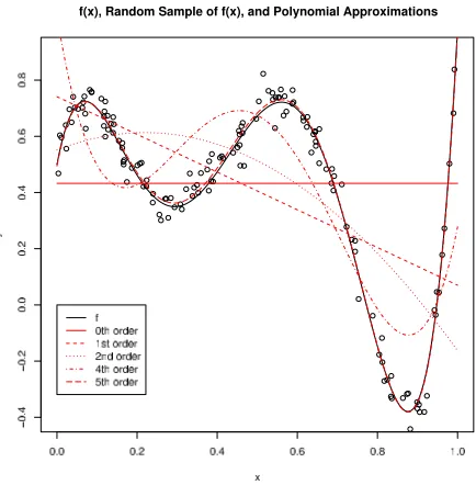
We consider the fifth-degree polynomial function
f(x) =.5(1−x) +150x(x−.25)(x−.3)(x−.75)(x−.95),
over the range x∈[0,1]. Figure 3 plots f , along with a 150 point data set drawn by choosing xi
uniformly in[0,1], and choosing y= f(x) +εi, whereεiis a Gaussian random variable with mean 0
and standard deviation .05. Figure 3 also shows (in red) the best polynomial approximations to the data (not to the ideal f ) of various orders. (We omit third order because it is nearly indistinguishable from second order.)
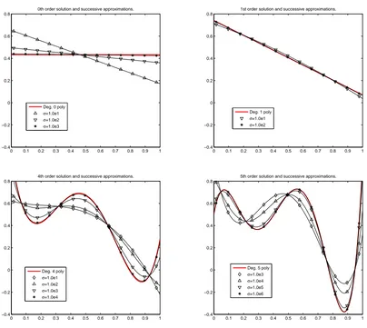
According to Theorem 14, if we parametrize our system by a variable s, and solve a Gaussian regularized least-squares problem withσ2=s2andλ=λs˜ −(2p+1)for some integer p, then, as s→∞,
we expect the solution to the system to tend to the pth-order data-based polynomial approximation to f . Asymptotically, the value of the constant ˜λdoes not matter, so we (arbitrarily) set it to be 1. Figure 4 demonstrates this result.
Figure 3: f(x) =.5(1−x) +150x(x−.25)(x−.3)(x−.75)(x−.95), a random data set drawn from
f(x)with added Gaussian noise, and data-based polynomial approximations to f .
cannot be obtained via many standard tools (e.g. MATLAB(TM)). We performed our experiments using CLISP, an implementation of Common Lisp that includes arithmetic operations on arbitrary-precision floating point numbers.
9. Discussion
We have shown, under mild technical conditions, that the minimizer of a Tikhonov regularization problem with a Gaussian kernel with bandwidth σ behaves, as σ→ ∞ and λ=λσ˜ −p, like the
degree-p polynomial that minimizes empirical risk (with some additional regularization on the de-gree p coefficients when p is an integer). Our approach rested on two key ideas, epi-convergence, which allowed us to make precise statements about when the limits of minimizers converges to the minimizer of a limit, and value-based learning, which allowed us to work in terms of the predicted functional values, yi, as opposed to the more common technique of working with the coefficients ci in a functional expansion of the form f(x) =∑iciK(x,xi). This in turn allowed us to avoid
dis-cussing the limits of the ci, which we do not know how to characterize.
0 0.1 0.2 0.3 0.4 0.5 0.6 0.7 0.8 0.9 1 −0.4
−0.2 0 0.2 0.4 0.6 0.8
0th order solution and successive approximations.
Deg. 0 poly σ=1.0e1 σ=1.0e2 σ=1.0e3
0 0.1 0.2 0.3 0.4 0.5 0.6 0.7 0.8 0.9 1 −0.4
−0.2 0 0.2 0.4 0.6 0.8
1st order solution and successive approximations.
Deg. 1 poly σ=1.0e1 σ=1.0e2
0 0.1 0.2 0.3 0.4 0.5 0.6 0.7 0.8 0.9 1 −0.4
−0.2 0 0.2 0.4 0.6 0.8
4th order solution and successive approximations.
Deg. 4 poly σ=1.0e1 σ=1.0e2 σ=1.0e3 σ=1.0e4
0 0.1 0.2 0.3 0.4 0.5 0.6 0.7 0.8 0.9 1 −0.4
−0.2 0 0.2 0.4 0.6 0.8
5th order solution and successive approximations.
Deg. 5 poly σ=1.0e3 σ=1.0e4 σ=1.0e5 σ=1.0e6
Figure 4: As s→∞, σ2=s2 andλ=s−(2k+1), the solution to Gaussian RLS approaches the kth order polynomial solution.
performance of a Bayesian weighted misclassification score. One can get some intuition about this tradeoff between smallerλand largerσby considering example 4 of Zhou (2002) where a tradeoff betweenσand R is seen for the covering numbers of balls in an RKHS induced by a Gaussian kernel (R can be thought of as roughly √1
λ).
We think it is interesting that some low-rank approximations to Gaussian kernel matrix-vector products (see Yang et al. (2005)) tend to work much better for large values ofσ. Our results raise the possibility that these low-rank approximations are merely recovering low-order polynomial be-havior; this will be a topic of future study.
requirement; it is possible to work with the pseudoinverse of K for finite-dimensional kernels (such as the dot-product kernel).
Acknowledgments
The authors would like to acknowledge Roger Wets and Adrian Lewis for patiently answering questions regarding epi-convergence. We would also like to thank our reviewers for their comments and suggestions.
Appendix A
In this appendix, we state and prove several matrix identities that we use in the main body of the paper.
Lemma 15 Let X,U∈Rm×m, Z,W ∈Rn×n, and Y,V ∈Rn×mwith
X Yt Y Z
symmetric, positive definite. If
U Vt V W
X Yt Y Z
=
Im 0
0 In
(15)
then
U = (X−YtZ−1Y)−1 (16) W−1V = −Y X−1 (17)
VU−1 = −Z−1Y (18)
W = (Z−Y X−1Yt)−1 (19) Proof Since
X Yt Y Z
, is symmetric, positive definite,
U Vt V W
is symmetric, positive definite,
as are X,Z,U,W .
Multiplying out (15) in block form,
U X+VtY = Im (20) V X+WY = 0 (21)
UYt+VtZ = 0 (22)
VYt+W Z = In (23)
Since U,W,X,Z are non-singular, (21) implies (17) and (22) implies (18). Substituting V=−Z−1YU
into (20) yields U X−UYtZ−1Y =U(X−YtZ−1Y) =Imand thus (16). Similarly, V =−WY X−1
and (23) give (19).
Lemma 16 Let
M=
A Bt Ct B D Et C E F
be symmetric positive definite. Let
M−1=
¯
A B¯t C¯t
¯
B D¯ E¯t
¯
C E¯ F¯
.
Then ¯D−E¯tF¯−1E¯ = (D−BA−1Bt)−1.
Proof By (16) of Lemma 15, on M with U=
A Bt B D
,
A Bt B D
−1
=
¯
A B¯t
¯
B D¯
− ¯ Ct ¯ Et ¯
F−1(C¯ E¯).
By (19) of Lemma 15, on
A Bt B D
,
A Bt B D
−1
=
··· ··· ··· (D−BA−1Bt)−1
.
Combining the lower-right blocks of the above two expansions yields the result.
Lemma 17 If
M=
A Bt Ct B D Et C E F
=
G 0 0
H J 0
K N P
G 0 0
H J 0
K N P
t
.
is symmetric positive definite, then JJt=D−BA−1Bt.
Proof Clearly
A Bt B D = G 0 H J G 0 H J t and thus
A=GGt, B=HGt, D=JJt+HHt
and hence JJt=D−HHt =D−BG−tG−1Bt =D−B(GGt)−1Bt =D−BA−1Bt. References
N. Aronszajn. Theory of reproducing kernels. Trans. Amer. Math. Soc., 68:337–404, 1950.
C. J. C. Burges and D. J. Crisp. Uniqueness of the svm solution. In Neural Information Processing
Systems, 1999.
Theodoros Evgeniou, Massimiliano Pontil, and Tomaso Poggio. Regularization networks and sup-port vector machines. Adv. In Comp. Math., 13(1):1–50, 2000.
S. Sathiya Keerthi and Chih-Jen Lin. Asymptotic behaviors of support vector machines with Gaus-sian kernel. Neural Computation, 15(7):1667–1689, 2003.
Ross A. Lippert and Ryan M. Rifkin. Asymptotics of gaussian regularized least squares. In Y. Weiss, B. Sch¨olkopf, and J. Platt, editors, Adv. in Neural Info. Proc. Sys. 18. MIT Press, Cambridge, MA, 2006.
R. Tyrrell Rockafellar and Roger J. B. Wets. Variational Analysis. Springer, Berlin, 2004.
Bernhard Sch¨olkopf, Ralf Herbrich, and Alex J. Smola. A generalized representer theorem. In 14th
Annual Conference on Computational Learning Theory, pages 416–426, 2001.
Grace Wahba. Spline Models for Observational Data, volume 59 of CBMS-NSF Regional
Confer-ence Series in Applied Mathematics. Soc. for Industrial & Appl. Math., 1990.
Grace Wahba, Yi Lin, Yoonkyung Lee, and Hao Zhang. On the relation between the GACV and Joachims’ ξα method for tuning support vector machines, with extensions to the non-standard case. Technical Report 1039, U. Wisconsin department of Statistics, 2001. URL
citeseer.ist.psu.edu/wahba01relation.html.
Changjiang Yang, Ramani Duraiswami, and Larry Davis. Efficient kernel machines using the im-proved fast gauss transform. In Lawrence K. Saul, Yair Weiss, and L´eon Bottou, editors,
Ad-vances in Neural Information Processing Systems 17, pages 1561–1568, Cambridge, MA, 2005.
MIT Press.