Learning Factor Graphs in Polynomial Time and Sample Complexity
Pieter Abbeel [email protected]
Daphne Koller [email protected]
Andrew Y. Ng [email protected]
Computer Science Department Stanford University
Stanford, CA 94305, USA
Editor: Sanjoy Dasgupta
Abstract
We study the computational and sample complexity of parameter and structure learning in graphical models. Our main result shows that the class of factor graphs with bounded degree can be learned in polynomial time and from a polynomial number of training examples, assuming that the data is generated by a network in this class. This result covers both parameter estimation for a known network structure and structure learning. It implies as a corollary that we can learn factor graphs for both Bayesian networks and Markov networks of bounded degree, in polynomial time and sample complexity. Importantly, unlike standard maximum likelihood estimation algorithms, our method does not require inference in the underlying network, and so applies to networks where inference is intractable. We also show that the error of our learned model degrades gracefully when the generating distribution is not a member of the target class of networks. In addition to our main result, we show that the sample complexity of parameter learning in graphical models has an O(1) dependence on the number of variables in the model when using the KL-divergence normalized by the number of variables as the performance criterion.1
Keywords: probabilistic graphical models, parameter and structure learning, factor graphs, Markov networks, Bayesian networks
1. Introduction
Graphical models are widely used to compactly represent structured probability distributions over (large) sets of random variables. Learning a graphical model from data is important for many applications. This learning problem can vary along several axes, including whether the data is fully or partially observed, and whether the structure of the network is given or needs to be learned from data.
In this paper, we focus on the problem of learning both network structure and parameters from fully observable data, restricting attention to discrete probability distributions over finite sets. We focus on the problem of learning a factor graph representation (Kschischang et al., 2001) of the distribution. Factor graphs subsume both Bayesian networks and Markov networks, in that every Bayesian network or Markov network can be written as a factor graph of (essentially) the same size.2
1. A preliminary version of some of this work was reported in Abbeel et al. (2005).
We provide a new parameterization of factor graph distributions, which forms the basis for our results. In this new parameterization, every factor is written as a product of probabilities over the variables in the factor and its neighbors. We will refer to such subsets of variables as “local subsets of variables.” These local subsets of variables are of size at most d2 for factor graphs of bounded degree d. Thus, for factor graphs of bounded degree d, the probabilities appearing in our new parameterization are over at most d2 variables and can be estimated efficiently from training examples.3Hence this new parameterization naturally leads to an algorithm that solves the parameter learning problem in closed-form by estimating the probabilities over these local subsets
of variables from training examples. We show that our closed-form estimation procedure results in a good estimate of the true distribution. More specifically, for factor graphs of bounded degree, if the generating distribution falls into the target class, we show that our estimation procedure returns an accurate solution—one of low KL-divergence from the true distribution—given a polynomial
number of training examples.
In contrast to our new parameterization, the factors in a factor graph (or a Markov network) are typically considered to have no probabilistic interpretation at all. One exception is the canonical parameterization used in the Hammersley-Clifford theorem for Markov networks (Hammersley and Clifford, 1971; Besag, 1974b). The Hammersley-Clifford canonical parameterization expresses the distribution as a product of probabilities over all variables. However, the number of different in-stantiations is exponential in the number of variables. Therefore such probabilities over all variables cannot be estimated accurately from a small number of training examples. As a consequence the Hammersley-Clifford canonical parameterization is not suited for parameter learning.
Our closed-form parameter learning algorithm is the first polynomial-time and polynomial sample-complexity parameter learning algorithm for factor graphs of bounded degree, and thereby for Markov networks of bounded degree. In contrast, we do not know how to do maximum like-lihood (ML) estimation in Markov networks or factor graphs without evaluating the likelike-lihood. Evaluating the likelihood is equivalent to evaluating the partition function. Evaluating the parti-tion funcparti-tion is known to be NP-hard, both exactly and approximately (Jerrum and Sinclair, 1993; Barahona, 1982). Indeed, all known exact algorithms grow exponentially in the tree-width of the graph, making the computation of the partition function intractable for many, even moderately sized, factor graphs. (See, for example, Cowell et al., 1999, for more details on such exact algorithms.) For example, n by n grids over binary variables (which have degree bounded by 4, independently of n) have tree-width n and the computational complexity of known algorithms for computing the partition function (and thus of known ML algorithms) is O(2n).
We analyze the sample complexity of parameter learning as a function of the number of variables in the network. We show that (under some mild assumptions) the sample complexity of parameter learning in graphical models has on O(1)dependence on the number of variables in the graphical model when using KL-divergence normalized by the number of variables as the performance crite-rion. This result is important since it gives theoretical support for the common practice of learning large graphical models from a relatively small number of training examples. More specifically, the number of training examples can be much smaller than the number of parameters when learning large graphical models.
(2001), for more details on the equivalence and conversion between factor graphs, Bayesian networks and Markov networks.
Building on our closed-form parameter learning algorithm, we provide an algorithm for learning not only the parameters, but also the structure. In our new parameterization, factors that are not present in the distribution can be computed in the same way from local probabilities as factors that are present in the distribution. As will become clear later, a key property of our new parameterization is that the factors not present in the distribution have all entries equal to one. This gives a very simple test to decide whether or not a factor is present in the distribution. Thus no iterative search procedure—as is common for most structure learning algorithms—is needed. However, to compute all the factors from local probabilities, we need to know which variables are its neighbors. So to complete the structure learning algorithm, we need to show how to find each factor’s neighbors. We show that local independence tests can be used to find the neighbors of each factor. Since local independence tests use statistics over a small number of variables only, the neighbors can be found efficiently from a small number of training examples.
Our structure learning algorithm provides the first polynomial-time and polynomial sample-complexity structure learning algorithm for factor graphs, and thereby for Markov networks. Note that our algorithm applies to any factor graph of bounded degree, including those (such as grids) where inference is intractable.
We also show that our algorithms degrade gracefully, in that they return reasonable answers even when the underlying distribution does not come exactly from the target class of networks.
We note that the proposed algorithms are unlikely to be useful in practice in their current form. The structure learning algorithm does an exhaustive enumeration over the possible neighbor sets of factors in the factor graph, a process which is—although polynomial—generally infeasible even in moderately sized networks. Both the parameter and the structure learning algorithm do not make good use of all the available data. Nevertheless, the techniques used in our analysis open new avenues towards efficient parameter and structure learning in undirected, intractable models.
The remainder of this paper is organized as follows. Section 2 provides necessary background about Gibbs distributions, the factor graph associated with a Gibbs distribution, Markov blankets and the Clifford canonical parameterization. In its original form, the Hammersley-Clifford theorem applies to Markov networks only. We provide an extension that applies to factor graphs. In Section 3, building on the canonical parameterization for factor graphs, we derive our novel parameterization, which forms the basis of our parameter estimation algorithm. We present our algorithm and provide formal running time and sample complexity guarantees. We conclude the section with an in-depth analysis of the relationship between the sample complexity and the number of random variables. In Section 4, we present our structure learning algorithm, and its formal guarantees. Section 5 discusses related work. For clarity of exposition, we provide the complete proofs of all theorems and propositions in the appendix.
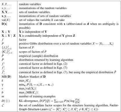
Table 1 gives an overview of the notation we use throughout this paper.
2. Preliminaries
X⋅
X X X
X X X
X X X
factor node
v ari ab l e node
X⋅
X X X
X X X
X X X
X X X
X X X
X X X
X X X
X X X
X X X
factor node
v ari ab l e node
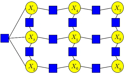
Figure 1: Example factor graph.
2.1 Gibbs Distributions
The probability distributions we consider are referred to as Gibbs distributions.
Definition 1 (Gibbs distribution) A factor f with scope4 D is a mapping from val(D)to R+. A
Gibbs distribution P over a set of random variables
X
={X1, . . . ,Xn} is associated with a set of factors{fj}Jj=1with scopes{Cj}Jj=1, such thatP(X1=x1, . . . ,Xn=xn) =
1
Z J
∏
j=1fj(Cj[x1, . . . ,xn]).
The normalizing constant Z is the partition function.
The factor graph associated with a Gibbs distribution is a bipartite graph whose nodes corre-spond to variables and factors, with an edge between a variable X and a factor fj if the scope of fj
contains X . There is one-to-one correspondence between factor graphs and the sets of scopes. Fig-ure 1 gives an example of a factor graph. Here the Gibbs distribution is over the variables X1,···,X9,
which are represented by circles in the factor graph. The factors are represented by squares and have the following respective scopes:{X1,X2,X3},{X1,X2},{X2,X3},{X1,X4},{X2,X5},{X3,X6},
{X4,X5},{X5,X6},{X4,X7},{X5,X8},{X7,X9},{X7,X8},{X8,X9}. The corresponding Gibbs
dis-tribution is given by
P(X1=x1,···,X9=x9) = 1
Z f{X1,X2,X3}(x1,x2,x3)f{X1,X2}(x1,x2)···f{X8,X9}(x8,x9).
A Gibbs distribution also induces a Markov network—an undirected graph whose nodes corre-spond to the random variables
X
and where there is an edge between two variables if there is a factor in which they both participate. The set of scopes uniquely determines the structure of the Markov network, but several different sets of scopes can result in the same Markov network. For example, a fully connected Markov network can correspond both to a Gibbs distribution with n2factors over pairs of variables, and to a distribution with a factor which is a joint distribution overX
. We willuse the more precise factor graph representation in this paper. Our results are easily translated into results for Markov networks.
Definition 2 (Markov blanket) Let a set of scopes
C
={Cj}Jj=1be given. The Markov blanket of a set of random variables D⊆X
is defined asMB(D) =∪{Cj: Cj∈
C
, Cj∩D6=/0} −D.Thus, the Markov blanket of a set of variables D is the minimal set of variables that separates D from the other variables in the factor graph. For the factor graph distribution of Figure 1 we have, for ex-ample, MB({X1}) ={X2,X3,X4}, MB({X1,X2}) ={X3,X4,X5}, and MB({X5}) ={X2,X4,X6,X8}.
For any Gibbs distribution, we have, for any subset of random variables D, that
D⊥
X
−D−MB(D) | MB(D), (1)or in words: given its Markov blanket MB(D), the set of variables D is independent of all other variables
X
−D−MB(D).5A standard assumption for a Gibbs distribution, which is critical for identifying its structure (see Lauritzen, 1996, Ch. 3), is that the distribution be positive—all of its entries be non-zero. Our results use a quantitative measure for how positive P is. Letγ=minx,iP(Xi=xi|
X
−i=x−i), wherethe−i subscript denotes all entries but entry i. Note that, if we have a fixed bound on the number
of factors in which a variable can participate, a fixed bound on the domain size for each variable, and a fixed bound on how skewed each factor is (more specifically a bound on the ratio of its lowest and highest entries), we are guaranteed a bound on γthat is independent of the number n of variables in the network. Thus, under these assumptions, our sample complexity results, which are expressed as a function of γ, have no hidden dependence on the number of variables n. In contrast, ˜γ=minxP(X=x) generally has an exponential dependence on n. For example, if we
have n independent and identically distributed (i.i.d.) Bernoulli(12) random variables, then γ= 1 2
(independent of n) but ˜γ= 1 2n.
2.2 The Canonical Parameterization
A Gibbs distribution is generally over-parameterized relative to the structure of the underlying fac-tor graph, in that a continuum of possible parameterizations over the graph can all encode the same distribution. The canonical parameterization (Hammersley and Clifford, 1971; Besag, 1974b) pro-vides one specific choice of parameterization for a Gibbs distribution, with some nice properties (see below). The canonical parameterization forms the basis for the Hammersley-Clifford theorem, which asserts that any distribution that satisfies the independence assumptions encoded by a Markov network can be represented as a Gibbs distribution with factors corresponding to each of the cliques in the Markov network. In its original formulation, the canonical distribution is defined for Gibbs distributions over Markov networks. We use a more refined parameterization, defined at the factor level; results at the clique level (or, equivalently, results for Markov networks) are trivial corollaries. The canonical parameterization is defined relative to an arbitrary (but fixed) set of “default” assignments ¯x= (x¯1, . . . ,x¯n). Let any subset of variables D=hXi1, . . . ,Xi|D|i, and any assignment
5. By X⊥Y we denote that X is independent of Y. By X⊥Y| Z we denote that X is conditionally independent of Y
d=hxi1, . . . ,xi|D|ibe given. Let any U⊆D be given. We defineσ·[·]such that for all i∈ {1, . . . ,n}:
(σU[d])i=
xi if Xi∈U,
¯
xi if Xi∈/U.
In words,σU[d]keeps the assignments to the variables in U as specified in d, and augments it to
form a full assignment using the default values in ¯x. Note that the assignments to variables outside U are always ignored, and replaced with their default values. Thus, the scope ofσU[·]is always U.
Let P be a positive Gibbs distribution.The canonical factor for D⊆
X
is defined as follows:fD∗(d) =exp ∑U⊆D(−1)|D−U|log P(σU[d])
. (2)
The sum is over all subsets of D, including D itself and the empty set /0.
The following theorem extends the Hammersley-Clifford theorem (which applies to Markov networks) to factor graphs.
Theorem 3 Let P be a positive Gibbs distribution with factor scopes {Cj}Jj=1. Let {C∗j}J
∗
j=1=
∪J
j=12Cj−/0(where 2Xis the power set of X—the set of all of its subsets). Then P(x) =P(¯x)∏J∗
j=1fC∗∗
j(c ∗
j),
where c∗j is the instantiation of C∗j consistent with x.
The proof is in the appendix.
The parameterization of P using the canonical factors{fC∗∗
j}
J∗
j=1is called the canonical param-eterization of P. Although typically J∗>J, the additional factors are all subfactors of the original
factors. Note that first transforming a factor graph into a Markov network and then applying the Hammersley-Clifford theorem to the Markov network generally results in a significantly less sparse canonical parameterization than the canonical parameterization from Theorem 3.
We now give an example to clarify the definition of canonical factors and canonical parameter-ization.
Example 1 Consider again the factor graph of Figure 1. Assume we take the fixed assignment to
be all zeros, namely we have ¯x1=0,x¯2=0,···,x¯9=0. Then the canonical factor f{∗X1,X2}over the variables X1,X2instantiated to x1,x2is given by
log f{∗X
1,X2}(x1,x2) = log P(X1=x1,X2=x2,X3=0,X4=0,···,X9=0) −log P(X1=0,X2=x2,X3=0,X4=0,···,X9=0)
−log P(X1=x1,X2=0,X3=0,X4=0,···,X9=0)
+log P(X1=0,X2=0,X3=0,X4=0,···,X9=0). (3)
So to compute the canonical factor, we start with the joint instantiation of the factor variables
Similarly, the canonical factor f{∗X
1,X2,X3}over the variables X1,X2,X3instantiated to x1,x2,x3is
given by
log f{∗X
1,X2,X3}(x1,x2,x3) = log P(X1=x1,X2=x2,X3=x3,X4=0,···,X9=0) −log P(X1=0,X2=x2,X3=x3,X4=0,···,X9=0)
−log P(X1=x1,X2=0,X3=x3,X4=0,···,X9=0)
−log P(X1=x1,X2=x2,X3=0,X4=0,···,X9=0) +log P(X1=0,X2=0,X3=x3,X4=0,···,X9=0) +log P(X1=0,X2=x2,X3=0,X4=0,···,X9=0)
+log P(X1=x1,X2=0,X3=0,X4=0,···,X9=0)
−log P(X1=0,X2=0,X3=0,X4=0,···,X9=0).
The canonical factor over just the variable X1instantiated to x1is given by
log f{∗X1}(x1) = log P(X1=x1,X2=0,X3=0,X4=0,···,X9=0)
−log P(X1=0,X2=0,X3=0,X4=0,···,X9=0).
Theorem 3 applied to our example gives the following expression for the probability distribution:
P(X1=x1,···,X9=x9) = P(X1=0,···,X9=0)
×f{∗X
1,X2,X3}(x1,x2,x3) ×f{∗X
1,X2}(x1,x2)f ∗
{X2,X3}(x2,x3)···f ∗
{X8,X9}(x8,x9) ×f{∗X1}(x1)f{∗X2}(x2)···f{∗X9}(x9)
= 1
Z
×f{∗X
1,X2,X3}(x1,x2,x3)
×f{∗X1,X2}(x1,x2)f{∗X2,X3}(x2,x3)···f{∗X8,X9}(x8,x9)
×f{∗X1}(x1)f{∗X2}(x2)···f{∗X9}(x9). (4)
3. Parameter Estimation
In this section we first introduce the parameter estimation ideas informally by expanding on Ex-ample 1. Then we formally introduce the key idea of Markov blanket canonical factors, which give a parameterization of a factor graph distribution only in terms of local probabilities. This new parameterization directly results in the proposed parameter estimation algorithm. We analyze the algorithm’s computational and sample complexity. In addition, we show an O(1)dependence on the number of variables in the network for the sample complexity when using the KL-divergence normalized by the number of variables in the network as performance criterion.
3.1 Parameter Estimation by Example
(and thus the distribution) in closed-form by estimating these probabilities from data. Unfortunately the probabilities appearing in the canonical factors are over full joint instantiations of all variables. As a consequence, these probabilities can not be estimated accurately from a small amount of data.
However, we will now consider the factor f{∗X
1,X2}more carefully and show it can be estimated from probabilities over small subsets of the variables only. The factor f{∗X
1,X2} contains an equal number of terms with positive and negative sign. For the sum of two such terms, we now derive a novel expression which contains local probabilities only (instead of probabilities of full joint instantiations of all variables).
log P(X1=x1,X2=x2,X3=0,X4=0,X5=0,X6=0,X7=0,X8=0,X9=0)
−log P(X1=x1,X2=0,X3=0,X4=0,X5=0,X6=0,X7=0,X8=0,X9=0) = log P(X1=x1,X2=x2|X3=0,X4=0,X5=0,X6=0,X7=0,X8=0,X9=0)
+log P(X3=0,X4=0,X5=0,X6=0,X7=0,X8=0,X9=0)
−log P(X1=x1,X2=0|X3=0,X4=0,X5=0,X6=0,X7=0,X8=0,X9=0)
−log P(X3=0,X4=0,X5=0,X6=0,X7=0,X8=0,X9=0)
= log P(X1=x1,X2=x2|X3=0,X4=0,X5=0,X6=0,X7=0,X8=0,X9=0)
−log P(X1=x1,X2=0|X3=0,X4=0,X5=0,X6=0,X7=0,X8=0,X9=0) = log P(X1=x1,X2=x2|MB({X1,X2}) =~0)
−log P(X1=x1,X2=0|MB({X1,X2}) =~0)
= log P(X1=x1,X2=x2|X3=0,X4=0,X5=0)
−log P(X1=x1,X2=0|X3=0,X4=0,X5=0). (5)
Here we used in order: the definition of conditional probability; same terms with opposite sign cancel; conditioning on the Markov blanket is equivalent to conditioning on all other variables; MB({X1,X2}) ={X3,X4,X5}in our example.
The last expression in Eqn. (5) contains local probabilities only, which can be estimated accu-rately from a small number of training examples. Using a similar reasoning as above for the other two terms of the factor f{∗X
1,X2}, we get the following expression for f ∗
{X1,X2}, which contains local probabilities only:
log f{∗X1,X2}(x1,x2) = log P(X1=x1,X2=x2|X3=0,X4=0,X5=0)
−log P(X1=x1,X2=0|X3=0,X4=0,X5=0)
−log P(X1=0,X2=x2|X3=0,X4=0,X5=0)
+log P(X1=0,X2=0|X3=0,X4=0,X5=0)
= log f{∗X
1,X2}|{X3,X4,X5}(x1,x2). (6)
The last line defines f{∗X
1,X2}|{X3,X4,X5}(x1,x2)(which we refer to as the Markov blanket canonical fac-tor for{X1,X2}). Although f{∗X
1,X2}(x1,x2) = f ∗
{X1,X2}|{X3,X4,X5}(x1,x2)when exact probabilities are used, we use different notation to explicitly distinguish how they are computed from probabilities. The Markov blanket canonical factor f{∗X
1,X2}|{X3,X4,X5}(x1,x2)is computed from local probabilities as given in Eqn. (6). The (original) canonical factor f{∗X
Similarly, the other canonical factors have equivalent Markov blanket canonical factors which involve local probabilities only. This gives us an efficient closed-form parameter estimation algo-rithm for our example. In the next few sections we formalize this idea for general factor graphs and analyze the computational and sample complexity.
3.2 Markov Blanket Canonical Factors
Considering the definition of the canonical parameters, we note that all of the terms in Eqn. (2) can be estimated from empirical data using simple counts, without requiring inference over the network. Thus, it appears that we can use the canonical parameterization as the basis for our parameter estimation algorithm. However, as written, this estimation process is statistically infeasible, as the terms in Eqn. (2) are probabilities over full instantiations of all variables, which can never be estimated from a reasonable number of training examples.
We now generalize our observation from the example in the previous section: namely, that we can express the canonical factors using only probabilities over much smaller instantiations—those corresponding to a factor and its Markov blanket. Let D=hXi1, . . . ,Xi|D|ibe any subset of variables,
and d=hxi1, . . . ,xi|D|ibe any assignment to D. For any U⊆D, we defineσU:D[d]to be the restriction
of the full instantiationσU[d]of all variables in
X
to the corresponding instantiation of the subset D.In other words,σU:D[d]keeps the assignments to the variables in U as specified in d, and changes
the assignment to the variables in D−U to the default values in ¯x. Let D⊆
X
and Y⊆X
−D. Then the factor fD∗|Yover the variables in D is defined as follows:fD∗|Y(d) =exp ∑U⊆D(−1)|D−U|log P(σ
U:D[d]|Y=¯y)
, (7)
where the sum is over all subsets of D, including D itself and the empty set /0. For example, we have that f{∗X
1,X2}|{X3,X4,X5}of the factor graph in Figure 1 is given by Eqn. (6) in the previous section.
The following proposition shows an equivalence between the factors computed using Eqn. (2) and Eqn. (7).
Proposition 4 Let P be a positive Gibbs distribution with factor scopes{Cj}Jj=1, and{C∗j}J
∗
j=1as above (i.e.,{C∗j}Jj∗=1=∪J
j=12Cj−/0). Then for any D⊆
X
, we have:fD∗= fD∗|X−D= fD∗|MB(D), (8)
and (as a direct consequence)
P(x) = P(¯x)∏J∗
j=1fC∗∗j|X−C∗j(c ∗
j) (9)
= P(¯x)∏J∗
j=1fC∗∗j|MB(C∗j)(c ∗
j), (10)
where c∗j is the instantiation of C∗j consistent with x.
Proposition 4 shows that we can compute the canonical parameterization factors using probabilities over factor scopes and their Markov blankets only. From a sample complexity point of view, this is a significant improvement over the standard definition which uses joint instantiations over all variables. Using Eqn. (7) we can expand the Markov blanket canonical factors in Proposition 4 and we see that any factor graph distribution can be parameterized as a product of local probabilities
X,Y, . . . random variables
x,y, . . . instantiations of the random variables X,Y, . . . sets of random variables
x,y, . . . instantiations of sets of random variables val(X) set of values the variable X can take
D[x] instantiation of D consistent with x (abbreviated as d when no ambiguity is
possible)
X⊥Y X is independent of Y
X⊥Y| Z X is conditionally independent of Y given Z
f factor
P positive Gibbs distribution over a set of random variables
X
=hX1, . . . ,Xni{fj}Jj=1 factors of P
{Cj}Jj=1 scopes of factors of P
ˆ
P empirical (sample) distribution
˜
P distribution returned by learning algorithm
f·∗ canonical factor as defined in Eqn. (2)
f·|·∗ canonical factor as defined in Eqn. (7) ˆ
f·|·∗ canonical factor as defined in Eqn. (7), but using the empirical distribution ˆP
MB(D) Markov blanket of D
k maxj|Cj|
γ minx,iP(Xi=xi|
X
−i=x−i)v maxi|val(Xi)|
b maxj|MB(Cj)|
m number of training examples
D(·k·) KL-divergence, D(PkQ) =∑x∈valXP(x)logQP((xx))
C
the set of candidate factor scopes for the structure learning algorithm,Factor-Graph-Structure-Learn(
C
={C∗j: C∗j ⊆X
,C∗j 6=/0,|C∗j| ≤k})Table 1: Notational conventions.
3.3 Parameter Estimation Algorithm
Based on the parameterization above, we propose the followingFactor-Graph-Parameter-Learn al-gorithm. The algorithm takes as inputs: the scopes of the factors {Cj}Jj=1, training examples
{x(i)}mi=1, a baseline instantiation ¯x. Then for {C∗j}Jj∗=1 as above (i.e., {C∗j}Jj∗=1=∪J
j=12Cj −/0),
Factor-Graph-Parameter-Learndoes the following:
• Compute the estimates of the canonical factors{fˆC∗∗
j|MB(C∗j)}
J∗
j=1as in Eqn. (7), but using the
empirical estimates based on the training examples.
• Return the probability distribution ˜P(x)∝ ∏J∗
j=1fˆC∗∗j|MB(C∗j)(c ∗
Theorem 5 (Parameter learning: computational complexity) The running time of the Factor-Graph-Parameter-Learnalgorithm is in O(m2kJ(k+b) +22kJvk).6
The proof is given in the appendix.
Note the representation of the factor graph distribution isΩ(Jvk), thus exponential dependence on k is unavoidable for any algorithm. More importantly, there is no dependence on the running time of evaluating the partition function. On the other hand, all currently known maximum likelihood estimation algorithms require evaluating the partition function, which is known to be NP-hard, both exactly and approximately (Jerrum and Sinclair, 1993; Barahona, 1982).
3.4 Sample Complexity
We now analyze the sample complexity of theFactor-Graph-Parameter-Learnalgorithm, showing that it returns a distribution that is a good approximation of the true distribution when given only a “small” number of training examples. We will use the sum of KL-divergences D(PkP˜) +D(P˜kP) to measure how well the distribution ˜P approximates the distribution P.7
Theorem 6 (Parameter learning: sample complexity) Let anyε,δ>0 be given. Let Factor-Graph-Parameter-Learnbe given (a) m training examples{x(i)}mi=1drawn i.i.d. from a distribution P and (b) the factor graph structure according to which the distribution P factors. Let ˜P be the probability distribution returned byFactor-Graph-Parameter-Learn. Then, we have that, for
D(PkP˜) +D(P˜kP)≤Jε
to hold with probability at least 1−δ, it suffices that the number of training examples m satisfies:
m≥(1+22kε+2)2 2 4k+3 γ2k+2bε2log2
k+2Jvk+b
δ . (11)
A complete proof is given in the appendix.
Theorem 6 shows that—assuming the true distribution P factors according to the given structure—
Factor-Graph-Parameter-Learnreturns a distribution that is Jε-close in KL-divergence. The sample complexity scales exponentially in the maximum number of variables per factor k, and polynomially in 1ε,1
γ.
The error in the KL-divergence grows linearly with the number of factors J. This is a con-sequence of the fact that the number of terms in the distributions is equal to the number of fac-tors J, and each term can accrue an error. We can obtain a more refined analysis if we elimi-nate this dependence by considering the KL-divergence normalized by the number of variables,
Dn(PkP˜) =1nD(PkP˜). We return to this topic in Section 3.5.
We now sketch the proof idea. The Markov blanket canonical factors are a product of local conditional probabilities. These local conditional probabilities can be estimated accurately from a “small” number of training examples. Thus the Markov blanket canonical factors can be estimated accurately from a small number of training examples. Thus the factor graph distribution—which is just a product of the Markov canonical factors—can be estimated accurately from a small number of training examples.
6. The upper bound is based on a very naive implementation’s running time. It assumes that operations on numbers (such as reading, writing, adding, etc.) take constant time.
7. D(PkQ) =∑x∈valXP(x)logP(
Theorem 6 considers the case when P factors according to the given structure. The following theorem shows that our error degrades gracefully even if the training examples are generated by a distribution Q that does not factor according to the given structure.
Theorem 7 (Parameter learning: graceful degradation) Let anyε,δ>0 be given. Let{x(i)}m i=1 be i.i.d. samples from a distribution Q. Let MB andMB be the Markov blankets according to thed
distribution Q and the given structure respectively. Let{fD∗∗
j|MB(D∗j)}
¯ J
j=1 be the non-trivial Markov blanket canonical factors of Q (those factors with not all entries equal to one). Let{C∗j}J∗
j=1be the scopes of the canonical factors in the factor graph given to the algorithm. Let ˜P be the probability distribution returned byFactor-Graph-Parameter-Learn. Then we have that for
D(QkP˜) +D(P˜kQ)≤Jε+2
∑
j:D∗j∈{/ C∗k}J∗ k=1 maxd∗j
log fD∗∗
j(d ∗
j)
+2
∑
j : MB(C∗j)6=dMB(C∗j) maxc∗j
log
fC∗∗
j|MB(C∗j)(c ∗
j)
f∗
C∗j|dMB(C∗j)(c∗j)
to hold with probability at least 1−δ, it suffices that the number of training examples m satisfies Eqn. (11) of Theorem 6.
Note the sample complexity depends on parameters k=maxj|C∗j|and b=maxj|MB(C∗j)|of the
given target structure (rather than the true structure). The graceful degradation result is important, as it shows that each canonical factor that is incorrectly captured by our target structure adds at most a constant (namely, l2l+1log1γ for an incorrectly captured factor over l variables) to our bound on the KL-divergence.8 This constant can be large, so we discuss the actual error contribution in more detail. A canonical factor could be incorrectly captured when the corresponding factor scope is not included in the given structure. Canonical factors are designed so that a factor over a set of variables captures only the residual interactions between the variables in its scope, once all interactions be-tween its subsets have been accounted for in other factors. Thus, canonical factors over large scopes are often close to the trivial all-ones factor in practice. Therefore, if our structure approximation is such that it only ignores some of the larger-scope factors, the error in the approximation may be quite limited. A canonical factor could also be incorrectly captured when the given structure does not have the correct Markov blanket for that factor. The resulting error depends on how good an approximation of the Markov blanket we do have. See Section 4 for more details on the error caused by incorrect Markov blankets.
3.5 Reducing the Dependence on Network Size
Our previous analysis showed a linear dependence of the sample complexity on the number of factors J in the network (for parameter learning). In a sense, this dependence is inevitable. To un-derstand why, consider a distribution P defined by a set of n independent Bernoulli random variables
X1, . . . ,Xn, each with parameter 0.5. Assume that Q is an approximation to P, where the Xiare still
independent, but have parameter 0.4999. Intuitively, a Bernoulli(0.4999) distribution is a very good
8. Each factor over l variables is a fraction of a product of 2l−1conditional probabilities over another product of 2l−1 conditional probabilities. Recall thatγ=minx,iP(Xi=xi|X−i=x−i)>0, so we have that each conditional probability
over l variables lies in the interval[γl,1]. Thus we have for a factor over l variables that maxd∗
j log fD∗∗
j(d
∗ j)
≤
log 1
γl2l−1 =l2
l−1log1
γ. Similarly, we have that maxc∗ j log
fC∗∗
j|MB(C∗j)(c ∗ j)
f∗
C∗j|dMB(C∗j)(c∗j)
estimate of a Bernoulli(0.5); thus, for most applications, Q can safely be considered to be a very good estimate of P. However, the KL-divergence D(P(X1:n)kQ(X1:n)) =∑ni=1D(P(Xi)kQ(Xi)) =
Ω(n). Thus, if n is large, the KL divergence between P and Q would be large, even though Q is a good estimate for P. To remove such unintuitive scaling effects when studying the dependence on the number of variables, we can consider instead the normalized KL divergence criterion:
Dn(P(X1:n)kQ(X1:n)) =n1D(P(X1:n)kQ(X1:n)).
As we now show, with a slight modification to the algorithm, we can achieve a bound ofεfor our normalized KL-divergence while eliminating the logarithmic dependence on J in our sample complexity bound. Specifically, we can modify our algorithm so that it clips probability estimates
∈[0,γk+b)toγk+b. The clipping procedure is motivated by the proof of Theorem 8 and effectively
ensures that the KL-divergence is bounded.9 Note that—since true probabilities which we are trying to estimate are never in the interval[0,γk+b)—this change can only improve the estimates.10
For this slightly modified version of the algorithm, the following theorem shows the dependence on the size of the network is O(1), which is tighter than the logarithmic dependence shown in Theorem 6.11
Theorem 8 (Parameter learning: size of the network) Let anyε,δ>0 be given and fixed. Let
{x(i)}mi=1be i.i.d. samples from P. Let the domain size of each variable be fixed. Let the degree of both the factor and variable nodes be bounded by a fixed constant. Letγ=minx,iP(Xi=xi|X−i= x−i)be fixed. Let ˜P be the probability distribution returned byFactor-Graph-Parameter-Learn. Then we have that, for
Dn(PkP˜) +Dn(P˜kP)≤ε
to hold with probability at least 1−δ, it suffices that we have a certain number of training examples that does not depend on the number of variables in the network.
The following theorem shows a similar result for Bayesian networks, namely that for a fixed bound on the number of parents per node, the sample complexity dependence on the size of the network is O(1).12
9. In particular, we first show that the error contribution from any fixed factor is small with high probability. Then— rather than using a Union bound to ensure the error contributions from all factors are small, which would result in a logarithmic dependence of the sample complexity on the number of factors (or variables)—we use Markov’s inequality to show that the error contribution of almost all factors is small with high probability. This leaves us to bound the error contribution of the (few) remaining factors, for which the error contribution is not small. By clipping the probability estimates, we can ensure their error contribution is bounded. A very similar reasoning applies to the case of Theorem 9. (See the proofs of Theorems 8 and 9, given in the appendix, for more details.)
10. This solution assumes thatγis known. If not, we can use a clipping threshold as a function of the number of training examples. Such an adaptive clipping procedure was used by Dasgupta (1997) to derive sample complexity bounds for learning fixed structure Bayesian networks.
11. We note that Theorem 8 assumes the maximum number of factors a variable can participate in is fixed (i.e., it cannot grow with the number of variables in the network). As a consequence, the dependence on the number of factors J and the dependence on the number of variables n are equivalent (up to a constant factor).
12. Complete proofs for Theorems 8 and 9 (and all other results in this paper) are given in the appendix of this paper. In the appendix we actually give a much stronger version of Theorem 9, including dependencies of m onε,δ,k and
Theorem 9 Let anyε>0 and δ>0 be given. Let any Bayesian network (BN) structure over n
variables with at most k parents per variable be given. Let P be a probability distribution that factors over the BN. Let ˜P denote the probability distribution obtained by fitting the conditional probability tables (CPT) entries via maximum likelihood and then clipping each CPT entry to the interval[8|valε(X
j)|3,1− ε
8|val(Xj)|3]. Then we have that for
Dn(PkP˜)≤ε
to hold with probability at least 1−δ, it suffices that we have a certain number of training examples that does not depend on the number of variables in the network.
Theorems 8 and 9 provide theoretical support for the common practice of learning large graph-ical models from a relatively small number of training examples. More specifgraph-ically, the number of training examples can be much smaller than the number of parameters when learning large graphical models. In contrast, for many problems in machine learning, the sample complexity grows roughly linearly or at most as some low-order polynomial in the number of parameters (Vapnik, 1998). The difference in sample complexity relates to the discussion of generative versus discriminative training. Indeed our result generalizes and even strengthens the results of Ng and Jordan (2002). They showed a logarithmic dependence on the number of variables for the very specific case of a graphical model with the naive Bayes structure.
4. Structure Learning
The algorithm described in the previous section uses the known network to establish a Markov blanket for each factor. This Markov blanket is then used to estimate the canonical parameters from empirical data. In this section, we show how we can build on this algorithm to perform structure learning, by first identifying (from the data) an approximate Markov blanket for each candidate factor, and then using this approximate Markov blanket to compute the parameters of that factor from a “small” number of training examples.
4.1 Identifying Markov Blankets
In the parameter learning results, the Markov blanket MB(C∗j) is used to efficiently estimate the conditional probability P(C∗j|X−C∗j), which is equal to P(C∗j|MB(C∗j)). This suggests to measure the quality of a candidate Markov blanket Y by how well P(C∗j|Y)approximates P(C∗j|
X
−C∗j). In this section we show how conditional entropy can be used to find a candidate Markov blanket that gives a good approximation for this conditional probability.13εsufficiently small, we have that naively clipping the probability estimates(0,0,1/4,3/4)to the interval(ε,1−ε)
results in(ε,ε,1/4,3/4), which does not sum to one (but rather to 1+2ε). Subtracting the additional probability mass 2εfrom the highest entry fixes this problem. For this example we get (ε,ε,1/4,3/4−2ε). In general, for
v-valued random variables, the probability estimates can be made to sum to one (after clipping) by subtracting at
most(v−1)εfrom the highest probability estimate. In the appendix we expand more on the topic of clipping for non-binary random variables.
Definition 10 (Conditional Entropy) Let P be a probability distribution over over X,Y. Then the
conditional entropy H(X|Y)of X given Y is defined as
−
∑
x∈val(X),y∈val(Y)
P(X=x,Y=y)log P(X=x|Y=y).
Proposition 11 (Cover & Thomas, 1991) Let P be a probability distribution over X,Y,Z. Then
we have H(X|Y,Z)≤H(X|Y).
Proposition 11 shows that conditional entropy can be used to find the Markov blanket for a given set of variables. Namely, let D,Y⊆
X
, D∩Y=/0, then we haveH(D|MB(D)) =H(D|
X
−D)≤H(D|Y), (12)where the equality follows from the Markov blanket property stated in Eqn. (1) and the inequality follows from Proposition 11. Thus, we can select the set of variables Y that minimizes H(D|Y)as our candidate Markov blanket for the set of variables D.
Our first difficulty is that, when learning from data, we do not have the true distribution, and hence the exact conditional entropies are unknown. The following lemma shows that the conditional entropy can be efficiently estimated from samples.
Lemma 12 Let P be a probability distribution over X,Y such that for all instantiations x,y we have
P(X=x,Y=y)≥λ. LetH be the conditional entropy computed based upon m i.i.d. samples fromb
P. Then for
H(X|Y)−Hb(X|Y)≤ε
to hold with probability 1−δ, it suffices that:
m≥8|val(Xλ)|22ε|2val(Y)|2log
4|val(X)||val(Y)|
δ .
However, as the empirical estimates of the conditional entropy are noisy, the true Markov blan-ket is not guaranteed to achieve the minimum of H(D|Y). In fact, in some probability distributions, many sets of variables could be arbitrarily close to reaching equality in Eqn. (12). Thus, in many cases, our procedure will not recover the actual Markov blanket, when given only a finite num-ber of training examples. Fortunately, as we show in the next lemma, any set of variables U∪W that is close to achieving equality in Eqn. (12) gives an accurate approximation P(Cj|U,W)of the
probabilities P(Cj|X−Cj)used in the canonical parameterization.
Lemma 13 Let anyε>0 be given. Let P be a distribution over disjoint sets of random variables U,V,W,X,Y. Letλ1=minu∈val(U),v∈val(V),w∈val(W)P(u,v,w), and let
λ2=minx∈val(X),u∈val(U),v∈val(V),w∈val(W)P(x|u,v,w). Assume the following holds:
X⊥Y,W | U,V, (13)
H(X|U,W)≤H(X|U,V,W,Y) +ε. (14)
Then we have that∀x,y,u,v,w
log P(x|u,v,w,y)−log P(x|u,w)≤λ√2ε
In other words, if a set of variables U∪W looks like a Markov blanket for X, as evaluated by the conditional entropy H(X|U,W), then the conditional distribution P(X|U,W)must be close to the conditional distribution P(X|X−X). Thus, it suffices to find such an approximate Markov blanket U∪W as a substitute for knowing the true Markov blanket U∪V. This makes conditional entropy suitable for structure learning.
4.2 Structure Learning Algorithm
We propose the followingFactor-Graph-Structure-Learnalgorithm. The algorithm receives as input: training examples {x(i)}mi=1; k: the maximum number of variables per factor; b: the maximum number of variables per Markov blanket for any set of variables up to size k; ¯x: a base instantiation.14
Let
C
be the set of candidate factor scopes, letY
be the set of candidate Markov blankets. I.e., we haveC
= {C∗j: C∗j ⊆X
,C∗j6= /0,|C∗j| ≤k}, (16)Y
= {Y : Y⊆X
,|Y| ≤b}. (17)The algorithm does the following:
• ∀C∗j ∈
C
, findMB(d C∗j) =arg minY∈Y,Y∩C∗j=/0Hb(C ∗
j|Y), which is the best candidate Markov
blanket.
• ∀C∗j ∈
C
, compute the estimates{fˆ∗ C∗j|MBd(C∗j)}
jof the canonical factors as defined in Eqn. (7)
using the empirical distribution.
• Threshold to one the factor entries ˆf∗
C∗j|dMB(C∗j)(c∗j)satisfying|log ˆfC∗∗j|MBd(C∗j)(c∗j)| ≤
ε
2k+2, and discard the factors that have all entries equal to one.
• Return the probability distribution ˜P(x)∝ ∏jfˆ∗
C∗j|dMB(C∗j) (c∗j).
The thresholding step finds the factors that actually contribute to the distribution. The specific threshold is chosen to suit the proof of Theorem 15. If no thresholding were applied, the error in Eqn. (18) would be |2Ck|εinstead of Jε, which is much larger in case the true distribution has a relatively small number of factors J.
Theorem 14 (Structure learning: computational complexity) The running time15 of Factor-Graph-Structure-Learnis in O mknkbnb(k+b) +knkbnbvk+b+knk2kvk.
Thus the running time is exponential in the maximum factor scope size k and the maximum Markov blanket size b, polynomial in the number of variables n and the maximum domain size v, and linear in the number of training examples m.
The first two terms in Theorem 14 result from going through the data and computing the em-pirical conditional entropies. Since the algorithm considers all combinations of candidate factors and Markov blankets, we have an exponential dependence on the maximum scope size k and the
14. Note in the parameter learning setting we had b equal to the size the largest Markov blanket for an actual factor in the distribution. In contrast, now b corresponds to the size of the largest Markov blanket for any candidate factor up to size k.
maximum Markov blanket size b. The last term comes from computing the Markov blanket canon-ical factors. Importantly, unlike for currently-known (exact) ML approaches, the running time does not depend on the tractability of inference in the (unknown) factor graph from which the data was sampled, nor on the tractability of inference in the recovered factor graph.
Theorem 15 (Structure learning: sample complexity) Let anyε,δ>0 be given. Let Factor-Graph-Structure-Learnbe given (a) m training examples{x(i)}mi=1 drawn i.i.d. from a distribution P, (b) an upper bound k on the number of variables per factor in the factor graph for P, and (c) an upper bound b on the number of variables per Markov blanket for any set of variables up to size k in the factor graph for P. Let ˜P be the distribution returned byFactor-Graph-Structure-Learn. Then for
D(PkP˜) +D(P˜kP)≤Jε (18)
to hold with probability 1−δ, it suffices that the number of training examples m satisfies:
m≥(1+εγ22kk++b3)2 v
2k+2b28k+19
γ6k+6bmin{ε2,ε4}log8kbn k+bvk+b
δ . (19)
Proof (sketch). From Lemmas 12 and 13 we have that the conditioning set chosen by Factor-Graph-Structure-Learn results in a good approximation of the true canonical factor. At this point the structure is fixed, and we can use the sample complexity theorem for parameter learning to finish the proof.
Theorem 15 shows that the sample complexity depends exponentially on the maximum factor size
k and the maximum Markov blanket size b; and polynomially on 1γ and1ε. If we modify the analysis to consider the normalized KL-divergence, as in Section 3.5, we obtain a logarithmic dependence on the number of variables in the network.
To understand the implications of this theorem, consider the class of Gibbs distributions where every variable can participate in at most d factors and every factor can have at most k variables in its scope. Then we have that the Markov blanket size b≤dk2. Bayesian network probability distributions can also be represented using factor graphs.16 If the number of parents per variable is bounded by numP and the number of children per variable is bounded by numC, then we have
k≤numP+1, and that b≤(numC+1)(numP+1)2. Thus our factor graph structure learning
algorithm allows us to efficiently learn distributions that can be represented by Bayesian networks with a bounded number of children and parents per variable. Note that our algorithm recovers a distribution which is close to the true generating distribution, but the distribution it returns is encoded as a factor graph, which may not be representable as a compact Bayesian network.
Theorem 15 considers the case where the generating distribution P factors according to a struc-ture with factor scope sizes bounded by k and size of Markov blankets (of any subset of variables of size less than k) bounded by b. As we did in the case of parameter estimation, we can show that we have graceful degradation of performance for distributions that do not satisfy these assumptions.
Theorem 16 (Structure learning: graceful degradation) Let anyε,δ>0 be given. Let{x(i)}m i=1 be training examples drawn i.i.d. from a distribution Q. Let MB and MB be the Markov blan-d
kets according to the distributions Q and found byFactor-Graph-Structure-Learnrespectively. Let
{fD∗∗
j|MB(D∗j)}j be the non-trivial Markov blanket canonical factors of Q (those factors with not all
entries equal to one). Let J be the number of non-trivial Markov blanket canonical factors in Q with scope size smaller than k. Let ˜P be the probability distribution returned by Factor-Graph-Parameter-Learn. Then we have that for
D(QkP˜) +D(P˜kQ) ≤ (J+|S|)ε+ 2
∑
j:|D∗j|>k
maxd∗j
log fD∗∗
j(dj)
+ 2
∑
C∗j∈C:|MB(C∗j)|>b maxc∗j
log
fC∗∗
j|MB(C∗j)(c ∗
j) f∗
C∗j|dMB(C∗j) (c∗j)
to hold with probability at least 1−δ, it suffices that the number of training examples m satisfies Eqn. (19) of Theorem 15. Here S={j : C∗j ∈ {/ Dl}l,|MB(C∗j)|>b} is the set that indexes over the subsets of variables of size smaller than k over which there is no factor in the true distribution and for which the Markov blanket in the true distribution is larger than b;
C
is the set of candidate factor scopesC
={C∗j : C∗j⊆X
,C∗j 6=/0,|C∗j| ≤k}.Theorem 16 shows that (similar to the parameter learning setting) each canonical factor that is not captured by our learned structure contributes at most a constant to our bound on the KL-divergence (namely l2l+1log1γ for a factor over l variables, see footnote 8 for details) to our bound on the KL-divergence. This bound on the error contribution can be large, so we discuss the actual error contribution in more detail. The reason a canonical factor is not captured could be two-fold. First, the scope of the factor could be too large. The paragraph after Theorem 7 discusses when the resulting error is expected to be small. Second, the Markov blanket of the factor could be too large. As shown in Lemma 13, a good approximate Markov blanket is sufficient to get a good approximation. So we can expect these error contributions to be small if the true distribution is mostly determined by interactions between small sets of variables.
Recall that the structure learning algorithm correctly clips all estimates of trivial canonical fac-tors to the trivial all-ones factor, when the structural assumptions are satisfied. I.e., trivial facfac-tors are correctly estimated as trivial if their Markov blanket is of size smaller than b. The additional term|S|εcorresponds to estimation error on the factors that are trivial in the true distribution but that have a Markov blanket of size larger than b, and are thus not correctly estimated and clipped to trivial all-ones factors.
5. Related Work
Target distribution True distribution Structure/Parameter Samples Time Graceful degradation Reference
ML tree any structure poly poly yes [1]
ML bounded tree-width any structure poly NP-hard yes [2]
Bounded tree-width same structure poly poly no [3]
Factor graph same parameter infinite convex no [4], [5]
Factor graph same parameter poly poly yes [6]
Factor graph same structure poly poly yes [6]
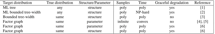
Table 2: Overview of prior work on learning Markov networks that has formal guarantees. More details are given in Section 5.1. The references in the table are: [1]: Chow and Liu (1968); [2] Srebro (2001); [3]: Narasimhan and Bilmes (2004); [4]: Besag (1974b); [5]: Gidas (1988); [6]: this paper. “Convex” refers to the time of solving a convex optimization problem.
5.1 Markov Networks
We split the discussion into two parts: parameter learning and structure learning.
5.1.1 PARAMETERLEARNING
The most natural algorithm for parameter estimation in undirected graphical models is maximum likelihood (ML) estimation (possibly with some regularization). Unfortunately, evaluating the like-lihood of such a model requires evaluating the partition function. All currently known ML algo-rithms for undirected graphical models require evaluating the partition function. Therefore, they are computationally tractable only for networks in which inference is computationally tractable. In contrast, our closed form solution can be efficiently computed from the data, even for Markov networks where inference is intractable. Note that our estimator does not return the ML solution, so that our result does not contradict the “hardness” of ML estimation. However, it does provide a low KL-divergence estimate of the probability distribution, with high probability, from a “small” number of training examples, assuming the true distribution approximately factors according to the given structure.
Criteria different from ML have been proposed for learning Markov networks. The most promi-nent one is pseudo-likelihood (Besag, 1974b), and its extension, generalized pseudo-likelihood (Huang and Ogata, 2002). The pseudo-likelihood criterion gives rise to a tractable convex opti-mization problem. Pseudo-likelihood estimation is consistent, that is, in the infinite sample limit it returns the true distribution, when the assumed structure is correct. (See, for example, Gidas, 1988, .) However, in the finite sample case the pseudo-likelihood estimate is often significantly worse than the maximum likelihood estimate. More information on the statistical efficiency of the pseudo-likelihood estimate can be found in, for example, Besag (1974a); Geyer and Thompson (1992); Guyon and K ¨unsch (1992). In contrast to our results, no finite sample bounds have been provided for pseudo-likelihood estimation. Moreover, the theoretical analyses (e.g., Geman and Graffigne, 1986; Comets, 1992; Guyon and K ¨unsch, 1992) only apply when the generating model is in the true target class.
5.1.2 STRUCTURELEARNING