Stagewise Lasso
Peng Zhao [email protected]
Bin Yu [email protected]
Department of Statistics University of Berkeley 367 Evans Hall
Berkeley, CA 94720-3860, USA
Editor: Saharon Rosset
Abstract
Many statistical machine learning algorithms minimize either an empirical loss function as in Ad-aBoost, or a penalized empirical loss as in Lasso or SVM. A single regularization tuning parameter controls the trade-off between fidelity to the data and generalizability, or equivalently between bias and variance. When this tuning parameter changes, a regularization “path” of solutions to the minimization problem is generated, and the whole path is needed to select a tuning parameter to optimize the prediction or interpretation performance. Algorithms such as homotopy-Lasso or LARS-Lasso and Forward Stagewise Fitting (FSF) (aka e-Boosting) are of great interest because of their resulted sparse models for interpretation in addition to prediction.
In this paper, we propose the BLasso algorithm that ties the FSF (e-Boosting) algorithm with the Lasso method that minimizes the L1penalized L2loss. BLasso is derived as a coordinate descent method with a fixed stepsize applied to the general Lasso loss function (L1penalized convex loss). It consists of both a forward step and a backward step. The forward step is similar to e-Boosting or FSF, but the backward step is new and revises the FSF (or e-Boosting) path to approximate the Lasso path. In the cases of a finite number of base learners and a bounded Hessian of the loss function, the BLasso path is shown to converge to the Lasso path when the stepsize goes to zero. For cases with a larger number of base learners than the sample size and when the true model is sparse, our simulations indicate that the BLasso model estimates are sparser than those from FSF with comparable or slightly better prediction performance, and that the the discrete stepsize of BLasso and FSF has an additional regularization effect in terms of prediction and sparsity. Moreover, we introduce the Generalized BLasso algorithm to minimize a general convex loss penalized by a general convex function. Since the (Generalized) BLasso relies only on differences not derivatives, we conclude that it provides a class of simple and easy-to-implement algorithms for tracing the regularization or solution paths of penalized minimization problems.
Keywords: backward step, boosting, convexity, Lasso, regularization path
1. Introduction
exponential loss function of the margin, while SVM a penalized hinge loss function of the margin. A single regularization tuning parameter, the number of iterations in AdaBoost and the smoothing parameter in SVM, controls the bias-and-variance trade-off or whether the algorithm overfits or un-derfits the data. When this tuning parameter changes, a regularization “path” of solutions to the minimization problem is generated. These algorithms have been shown to achieve start-of-the-art prediction performance. A tuning parameter value, or equivalently a point on the path of solutions, is chosen to minimize the estimated prediction error over a proper test set or through cross-validation. Hence it is necessary to have algorithms that can generate the path of solutions in an efficient man-ner. Path following algorithms have also been devised in other statistical penalized minimization problems such as the problems of information bottleneck Tishby et al. (1999) and information dis-tortion Gedeon et al. (2002) where the loss and penalty functions are different from these discussed in this paper. In fact, following the solution paths of numerical problems is the focus of homo-topy, a sub-area in numerical analysis. Interested readers are referred to the book Allgower and Georg (1980) (http://www.math.colostate.edu/emeriti/georg/AllgGeorgHNA.pdf) and references at http://www.math.colostate.edu/emeriti/georg/georg.publications.html.
Among all the machine learning methods, those that produce sparse models are of great inter-est because sparse models lend themselves more easily to interpretation and therefore preferred in sciences and social sciences. Lasso (Tibshirani, 1996) is such a method. It minimizes the L2 loss function with an L1penalty on the parameters in a linear regression model. In signal processing it is called Basis Pursuit (Chen and Donoho, 1994). The L1 penalty leads to sparse solutions, that is, there are few predictors or basis functions with nonzero weights (among all possible choices). This statement is proved asymptotically under various conditions by different authors (see, e.g., Knight and Fu, 2000; Osborne et al., 2000a,b; Donoho et al., 2006; Donoho, 2006; Rosset et al., 2004; Tropp, 2006; Zhao and Yu, 2006; Zou, 2006; Meinshausen and Yu, 2006; Zhang and Huang, 2006). Sparsity has also been observed in the models generated by Forward Stagewise Fitting (FSF) or e-Boosting. FSF is a gradient descent procedure with more cautious steps than L2Boosting (i.e., the usual coordinatewise gradient descent method applied to the L2loss) (Rosset et al., 2004; Hastie et al., 2001; Efron et al., 2004). Moreover, these papers also study the similarities between FSF (e-Boosting) with Lasso. This link between Lasso and e-Boosting or FSF is more formally described for the linear regression case through the LARS algorithm (Least Angle Regression Efron et al., 2004). It is also shown in Efron et al. (2004) that for special cases (such as orthogonal designs) e-Boosting or FSF can approximate Lasso path infinitely close, but in general, it is unclear what regularization criterion e-Boosting or FSF optimizes. As can be seen in our experiments (Figure 1 in Section 6.1), e-Boosting or FSF solutions can be significantly different from the Lasso solutions in the case of strongly correlated predictors which are common in high-dimensional data prob-lems. However, FSF is still used as an approximation to Lasso because it is often computationally prohibitive to solve Lasso with general loss functions for many regularization parameters through Quadratic Programming.
innovative “backward” step. This step uses the same minimization rule as the forward step to define each fitting stage but with an extra rule to force the model complexity or L1 penalty to decrease. By combining backward and forward steps, BLasso is able to go back and forth to approximate the Lasso path correctly.
BLasso can be seen as a marriage between two families of successful methods. Computationally, BLasso works similarly to e-Boosting and FSF. It isolates the sub-optimization problem at each step from the whole process, that is, in the language of the Boosting literature, each base learner is learned separately. This way BLasso can deal with different loss functions and large classes of base learners like trees, wavelets and splines by fitting a base learner at each step and aggregating the base learners as the algorithm progresses. Moreover, the solution path of BLasso can be shown to converge to that of the Lasso, which uses explicit global L1 regularization for cases with a finite number of base learners. In contrast, e-Boosting or FSF can be seen as local regularization in the sense that at any iteration, FSF with a fixed small stepsize only searches over those models which are one small step away from the current one in all possible directions corresponding to the base learners or predictors (cf. Hastie et al., 2006, for a recent interpretation of theε→0 case).
In particular, we make three contributions in this paper via BLasso. First, by introducing the backward step we modify e-Boosting or FSF to follow the Lasso path and consequently generate models that are sparser with equivalent or slightly better prediction performance in our simulations (with true sparse models and more predictors than the sample size). Secondly, by showing conver-gence of BLasso to the Lasso path, we further tighten the conceptual ties between e-Boosting or FSF and Lasso that have been considered in previous works. Finally, since BLasso can be generalized to deal with other convex penalties and does not use any derivatives of the Loss function or penalty, we provide the Generalized BLasso algorithm as a simple and easy-to-implement off-the-shelf method for approximating the regularization path for a general loss function and a general convex penalty.
We would like to note that, for the original Lasso problem, that is, the least squares problem (L2 loss) with an L1penalty, algorithms that give the entire Lasso path have been established, namely, the homotopy method by Osborne et al. (2000b) and the LARS algorithm by Efron et al. (2004). For parametric least squares problems where the number of predictors is not large, these methods are very efficient as their computational complexity is on the same order as a single Ordinary Least Squares regression. For other problems such as classification and for nonparametric setups like model fitting with trees, FSF or e-Boosting has been used as a tool for approximating the Lasso path (Rosset et al., 2004). For such problems, BLasso operates in a similar fashion as FSF or e-Boosting but, unlike FSF, BLasso can be shown to converge to the Lasso path quite generally when the stepsize goes to zero.
effect of using moderate stepsizes. Finally, Section 7 is a discussion and a summary. In particular, it comments on the computational complexity of BLasso, compares with the algorithm in Rosset (2004), explores the possibility of BLasso for nonparametric learning problems, summarizes the paper, and points to future directions.
2. Boosting, Forward Stagewise Fitting and the Lasso
Boosting was originally proposed as an iterative fitting procedure that builds up a model sequentially using a weak or base learner and then carries out a weighted averaging (Schapire, 1990; Freund, 1995; Freund and Schapire, 1996). More recently, boosting has been interpreted as a gradient descent algorithm on an empirical loss function. FSF or e-Boosting can be viewed as a gradient descent with a fixed small stepsize at each stage and it produces solutions that are often close to the Lasso solutions (path). We now give a brief gradient descent view of Boosting and of FSF (e-Boosting), followed by a review of the Lasso minimization problem.
2.1 Boosting and Forward Stagewise Fitting
Given data Zi= (Yi,Xi)(i=1, ...,n), where the univariate Y can be continuous (regression problem)
or discrete (classification problem), our task is to estimate the function F : Rd→R that minimizes an expected loss
E[C(Y,F(X))], C(·,·): R×R→R+.
The most prominent examples of the loss function C(·,·)include exponential loss (AdaBoost), logit loss and L2loss.
The family of F(·)being considered is the set of ensembles of “base learners”
D={F : F(x) =
∑
j
βjhj(x),x∈Rd,βj∈R},
where the family of base learners can be very large or contain infinite members, for example, trees, wavelets and splines.
Letβ= (β1, ...βj, ...)T, we can re-parametrize the problem using
L(Z,β):=C(Y,F(X)),
where the specification of F is hidden by L to make our notation simpler. To find an estimate forβ, we set up an empirical minimization problem:
ˆ
β=arg min
β n
∑
i=1
L(Zi;β).
(ˆj,gˆ) = arg min
j,g n
∑
i=1
L(Zi; ˆβt+g1j), (1)
ˆ
βt+1 = βˆt+g1ˆ
ˆj, (2)
where 1j is the jth standard basis vector with all 0’s except for a 1 in the jth coordinate, and g∈R
is stepsize. In other words, Boosting favors the direction ˆj that reduces most the empirical loss and ˆ
g is found through a line search. The well-known AdaBoost, LogitBoost and L2Boosting can all be viewed as implementations of this strategy for different loss functions.
Forward Stagewise Fitting (FSF) (Efron et al., 2004) is a similar method for approximating the minimization problem described by (1) with some additional regularization. FSF has also been called e-Boosting forε-Boosting as in Rosset et al. (2004). Instead of optimizing the stepsize as in (2), FSF updates ˆβt by a fixed stepsizeεas in Friedman (2001).
For general loss functions, FSF can be defined by removing the minimization over g in (1):
(ˆj,sˆ) = arg min
j,s=±ε
n
∑
i=1
L(Zi; ˆβt+s1j), (3)
ˆ
βt+1 = βˆt+s1ˆ
ˆj. (4)
This description looks different from the FSF described in Efron et al. (2004), but the underlying mechanic of the algorithm remains unchanged (see Section 5). Initially all coefficients are zero. At each successive step, a basis function or predictor or coordinate is selected that reduces most the empirical loss. Its corresponding coefficient βˆj is then incremented or decremented by a fixed amountε, while all other coefficientsβj, j6= ˆj are left unchanged.
By taking small steps, FSF imposes some local regularization or shrinkage. A related approach can be found in Zhang (2003) where a relaxed gradient descent method is used. After T <∞ iterations, many of the estimated coefficients by FSF will be zero, namely those that have yet to be incremented. The others will tend to have absolute values smaller than the unregularized solutions. This shrinkage/sparsity property is reflected in the similarity between the solutions given by FSF and Lasso which is reviewed next.
2.2 General Lasso
Let T(β)denote the L1penalty ofβ= (β1, ...,βj, ...)T, that is, T(β) =kβk1=∑j|βj|, andΓ(β;λ)
denote the Lasso (least absolute shrinkage and selection operator) loss function
Γ(β;λ) =
n
∑
i=1
L(Zi;β) +λT(β).
The general Lasso estimate ˆβ= (βˆ1, ...,βˆj, ...)T is defined by
ˆ
βλ=min
β Γ(β;λ).
very large λ will completely shrink ˆβ to 0 thus leading to the empty or null model. In general, moderate values of λwill cause shrinkage of the solutions towards 0, and some coefficients may end up being exactly 0. This sparsity in Lasso solutions has been researched extensively in recent years (e.g., Osborne et al., 2000a,b; Efron et al., 2004; Donoho et al., 2006; Donoho, 2006; Tropp, 2006; Rosset et al., 2004; Meinshausen and B ¨uhlmann, 2005; Candes and Tao, 2007; Zhao and Yu, 2006; Zou, 2006; Wainwright, 2006; Meinshausen and Yu, 2006; Zhang and Huang, 2006). Sparsity can also result from other penalties as in, for example, Fan and Li (2001).
Computation of the solution to the Lasso problem for a fixed λ has been studied for special cases. Specifically, for least squares regression, it is a quadratic programming problem with linear inequality constraints; for 1-norm SVM, it can be transformed into a linear programming problem. But to get a model that performs well on future data, we need to select an appropriate value for the tuning parameterλ. Very efficient algorithms have been proposed to give the entire regularization path for the squared loss function (the homotopy method by Osborne et al. 2000b and similarly LARS by Efron et al. 2004) and SVM (1-norm SVM by Zhu et al., 2003).
However, it remains open how to give the entire regularization path of the Lasso problem for general convex loss function. FSF exists as a compromise since, like Boosting, it is a nonparamet-ric learning algorithm that works with different loss functions and large numbers of base learners (predictors) but it is local regularization and does not converge to the Lasso path in general. As can be seen in Sec. 6.2, FSF has also less sparse solutions comparing to Lasso in our simulations.
Next we propose the BLasso algorithm which works in a computationally efficient fashion as FSF. In contrast to FSF, BLasso converges to the Lasso path for general convex loss functions when the stepsize goes to 0. This relationship between Lasso and BLasso leads to sparser solutions for BLasso comparing to FSF with similar or slightly better prediction performance in our simulation set-up with different choices of the stepsize.
3. The BLasso Algorithm
We first describe the BLasso algorithm (Algorithm 1). This algorithm has two related input param-eters, a stepsizeεand a tolerance levelξ.
The tolerance level is needed only to avoid numerical instability when assessing changes of the empirical loss function and should be set as small as possible while accommodating the numerical accuracy of the implementation. (ξis set to 10−6in the implementation of the algorithm that used in this paper.)
We will discuss forward and backward steps in depth in the next section. Immediately, the fol-lowing properties can be proved for BLasso (see Appendix for the proof).
Lemma 1.
1. For anyλ≥0, if there exist j and s with|s|=εsuch thatΓ(s1j;λ)≤Γ(0;λ), we haveλ0≥λ.
2. For any t, we haveΓ(βˆt+1;λt)≤Γ(βˆt;λt)−ξ.
3. Forξ≥0 and any t such thatλt+1<λt, we haveΓ(βˆt±ε1
j;λt)>Γ(βˆt;λt)−ξfor every j
andkβˆt+1k1=kβˆtk1+ε.
Algorithm 1 BLasso
Step 1 (initialization). Given data Zi= (Yi,Xi), i=1, ...,n and a small stepsize constantε>0 and a
small tolerance parameterξ>0, take an initial forward step
(ˆj,sˆˆj) = arg min
j,s=±ε
n
∑
i=1
L(Zi; s1j),
ˆ
β0 = sˆ ˆj1ˆj, Then calculate the initial regularization parameter
λ0=1 ε(
n
∑
i=1
L(Zi; 0)− n
∑
i=1
L(Zi; ˆβ0)).
Set the active index set IA0={ˆj}. Set t=0.
Step 2 (Backward and Forward steps). Find the “backward” step that leads to the minimal empirical loss:
ˆj=arg min
j∈IAt
n
∑
i=1
L(Zi; ˆβt+sj1j) where sj=−sign(βˆtj)ε. (5)
Take the step if it leads to a decrease of moderate sizeξin the Lasso loss, otherwise force a forward step (as (3), (4) in FSF) and relaxλif necessary:
IfΓ(βˆt+sˆ
ˆj1ˆj;λt)−Γ(βˆt,λt)≤ −ξ, then ˆ
βt+1=βˆt+sˆ
ˆj1ˆj,λt+1=λt. Otherwise,
(ˆj,sˆ) = arg min
j,s=±ε
n
∑
i=1
L(Zi; ˆβt+s1j), (6)
ˆ
βt+1 = βˆt+s1ˆ
ˆj, λt+1 = min[λt,1
ε(
n
∑
i=1
L(Zi; ˆβt)− n
∑
i=1
L(Zi; ˆβt+1)−ξ)],
IAt+1 = IAt ∪ {ˆj}.
Step 3 (iteration). Increase t by one and repeat Step 2 and 3. Stop whenλt ≤0.
Theorem 1. For a finite number of base learners and ξ=o(ε), if ∑L(Zi;β)is strongly convex
with bounded second derivatives inβthen asε→0, the BLasso path converges to the Lasso path uniformly.
Note that Conjecture 2 of Rosset et al. (2004) follows from Theorem 1. This is because if all the optimal coefficient paths are monotone, then BLasso will never take a backward step, so it will be equivalent to e-Boosting.
Many popular loss functions, for example, squared loss, logistic loss, and negative log-likelihood functions of exponential families are convex and twice differentiable, and they satisify the condi-tions in Theorem 1. Moreover, from the proof of this theorem in the appendix, it is easy to see that it suffices to have the conditions in the theorem satisfied over a bounded set ofβ. For the ex-ponential loss, Lemma 1 implies that there is a finiteλ0<∞for every data set(Zi). Thus we can
restrict the proof of Theorem 1 to this bounded set ofβto show the result for the exponential loss. Other functions like the hinge loss (SVM) is continuous and convex but not differentiable. The differentiability, however, is only necessary for the proof of Theorem 1. BLasso does not use any gradient or higher order derivatives but only the differences of the loss function therefore remains applicable to loss functions that are not differentiable or of which differentiation is too complex or computationally expensive. It is theoretically possible that BLasso’s coordinate descent strategy gets stuck at nondifferentiable points for functions like the hinge loss. However, as illustrated in our third experiment, BLasso may still work for cases like 1-norm SVM empirically.
Theorem 1 does not cover nonparametric learning problems with an infinite number of base learners either. In fact, for problems with large or infinite number of base learners, the minimization in (6) is usually done approximately by functional gradient descent and a toleranceξ>0 needs to be chosen to avoid oscillation between forward and backward steps caused by slow descending. We discuss more on this topic in the discussion (Sec. 7).
4. The Backward Step
We now explain the motivation and working mechanic of BLasso. Observe that FSF only uses “forward” steps, that is, it only takes steps that lead to a direct reduction of the empirical loss. Comparing to classical model selection methods like Forward Selection and Backward Elimination, Growing and Pruning of a classification tree, a “backward” counterpart is missing. Without the backward step, when FSF picks up more irrelevant variables as compared to the Lasso path in some cases (cf. Figure 1 in Section 6.2), it does not have a mechanism to remove them. As seen below, this backward step naturally arises in BLasso because of our coordinate descent view of the minimization of the Lasso loss. (Sinceξ exists for numerical purpose only, it is assumed to be 0 thus excluded in the following theoretical discussion.)
For a givenβ6=0 andλ>0, consider the impact of a smallε>0 change ofβjto the Lasso loss
Γ(β;λ). For an|s|=ε,
∆jΓ(Z;β) = ( n
∑
i=1
L(Zi;β+s1j)− n
∑
i=1
L(Zi;β)) +λ(T(β+s1j)−T(β))
:= ∆j( n
∑
i=1
L(Zi;β)) +λ∆jT(β).
∆jT(β) = kβ+s1jk1− kβk1=|βj+s| − |βj|
= ε·sign+(βj,s) (7)
= ε·
1 if sβj >0 orβj=0
-1 if sβj<0
.
Equation (7) shows that an εstep changes the penalty by a fixed εin absolute value for any j. That is, only the sign of the penalty change may vary. In the beginning of BLasso, all j directions are leaving zero and hence changing the L1penalty by the same positive amountλ·ε. Therefore the first step of BLasso is a forward step because minimizing Lasso loss is equivalent to minimizing the L2loss due to the same positive change of the L1 penalty. As the algorithm proceeds, some of the penalty changes might become negative and minimizing the empirical loss is no longer equivalent to minimizing the Lasso loss. In fact, except for special cases like orthogonal covariates (predictors), the FSF steps might result in negative changes of the L1penalty. In some of these situations, a step that goes “backward” reduces the penalty with a small sacrifice in the empirical loss. In general, to minimize the Lasso loss, one needs to go “back and forth” to trade off the penalty with the empirical loss for different regularization parameters.
To be precise, for a given ˆβ, a backward step is such that:
∆βˆ =sj1j,subject to ˆβj6=0,sign(s) =−sign(βˆj)and|s|=ε.
Making such a step will reduce the penalty by a fixed amountλ·ε, but its impact on the empirical loss can be different, therefore as in (5) we want:
ˆj=arg min
j n
∑
i=1
L(Zi; ˆβ+sj1j)subject to ˆβj6=0 and sj=−sign(βˆj)ε,
that is, ˆj is selected such that the empirical loss after making the step is as small as possible. While forward steps try to reduce the Lasso loss through minimizing the empirical loss, the backward steps try to reduce the Lasso loss through minimizing the Lasso penalty. In summary, by allowing the backward steps, we are able to work with the Lasso loss directly and take backward steps to correct earlier forward steps that might have picked up irrelevant variables.
Since much of the discussion on the similarity and difference between FSF and Lasso is focused on Least Squares problems (e.g., Efron et al., 2004; Hastie et al., 2001), we next examine the BLasso algorithm in this case. It is straightforward to see that in LS problems both forward and backward steps in BLasso are based only on the correlations between fitted residuals and the covariates (pre-dictors). It follows that BLasso in this case reduces to finding the best direction in both forward and backward steps by examining the inner-products, and then deciding whether to go forward or back-ward based on the regularization parameter. This not only simplifies the minimization procedure but also significantly reduces the computation complexity for a large number of observations since the inner-product betweenηt and Xj can be updated by
(ηt+1)0Xj= (ηt−sXˆjt)0Xj= (ηt)0Xj−sX0ˆjtXj, (8)
which takes only one operation if X0ˆjtXj is precalculated. Therefore, when the number of base
complexity independent from the number of observations. This nice property is not surprising as it is also observed in established algorithms like LARS and Osborne’s homotopy method which are specialized for LS problems.
In nonparametric situations, the number of base learners is large therefore the aforementioned strategy becomes inefficient. BLasso has a natural extention to this case as follows: similar to boost-ing, the forward step is carried out by a sub-optimization procedure such as fitting trees, smoothing splines or stumps. For the backward step, only inner-products between base learners that have en-tered the model need to be calculated. The inner products between these base learners and residuals can be updated by (8). This makes the backward steps’ computation complexity proportional to the number of base learners that are already chosen instead of the number of all possible base learners. Therefore BLasso works not only for cases with large sample size but also for cases where a class of large or infinite number of possible base learners is given.
As mentioned earlier, there are already established efficient algorithms for solving the least square (L2) Lasso problem, for example, the homotopy method by Osborne et al. (2000b) and LARS (Efron et al., 2004). These algorithms are very efficient for giving the exact Lasso paths for parametric settings. For nonparametric learning problems with a large or an infinite number of base learners, we believe BLasso is an attractive strategy for approximating the path of the Lasso, as it shares the same computational strategy as Boosting which has proven itself successful in ap-plications. Also, in cases where the Ordinary Least Square (OLS) method performs well, BLasso can be modified to start from the OLS estimate, go backward and stop in a few iterations.
5. Generalized BLasso
As stated earlier, BLasso not only works for general convex loss functions, but also extends to convex penalties other than the L1 penalty. For the Lasso problem, BLasso does a fixed stepsize coordinate descent to minimize the penalized loss. Since the penalty has the special L1 norm and (7) holds, a step’s impact on the penalty has a fixed size ε with either a positive or a negative sign, and the coordinate descent takes form of “backward” and “forward” steps. This reduces the minimization of the penalized loss function to unregularized minimizations of the loss function as in (6) and (5). For general convex penalties, since a step on different coordinates does not necessarily have the same impact on the penalty, one is forced to work with the penalized function directly. Assume T(β): Rm→R is a convex penalty function. We next describe the Generalized BLasso algorithm (Algorithm 2).
In the Generalized BLasso algorithm, explicit “forward” or “backward” steps are no longer seen. However, the mechanism remains the same—minimize the penalized loss function for eachλ, relax the regularization by reducingλthrough a “forward” step when the minimum of the loss function for the currentλis reached.
6. Experiments
Algorithm 2 Generalized BLasso
Step 1 (initialization). Given data Zi = (Yi,Xi), i=1, ...,n and a fixed small stepsizeε>0 and a
small tolerance parameterξ≥0, take an initial forward step
(ˆj,sˆˆj) =arg min
j,s=±ε
n
∑
i=1
L(Zi; s1j),βˆ0=sˆˆj1ˆj.
Then calculate the corresponding regularization parameter
λ0=∑ni=1L(Zi; 0)−∑ni=1L(Zi; ˆβ0)
T(βˆ0)−T(0) . Set t=0.
Step 2 (steepest descent on Lasso loss). Find the steepest coordinate descent direction on the penal-ized loss:
(ˆj,sˆˆj) =arg min
j,s=±εΓ( ˆ βt+s1
j;λt).
Update ˆβ if it reduces Lasso loss by at least a ξ amount, otherwise force ˆβ to minimize L and recalculate the regularization parameter:
IfΓ(βˆt+sˆ
ˆj1ˆj;λt)−Γ(βˆt,λt)<−ξ, then ˆ
βt+1=βˆt+sˆ
ˆj1ˆj,λt+1=λt. Otherwise,
(ˆj,sˆˆj) = arg min
j,|s|=ε
n
∑
i=1
L(Zi; ˆβt+s1j),
ˆ
βt+1 = βˆt+sˆ
ˆj1ˆj,
λt+1 = min[λt,∑ni=1L(Zi; ˆβt)−∑ni=1L(Zi; ˆβt+1)
T(βˆt+1)−T(βˆt) ].
Step 3 (iteration). Increase t by one and repeat Step 2 and 3. Stop whenλt ≤0.
same as the Lasso path which shrinks the added irrelevant variable back to zero, while FSF’s path parts drastically from Lasso’s due to the added strongly correlated covariate and does not move it back to zero.
The last experiment is to illustrate BLasso as an off-the-shelf method for computing the reg-ularization path for general convex loss functions and general convex penalties. Two cases are presented. The first case is bridge regression (Frank and Friedman, 1993) on diabetes data using different Lγ(γ≥1) norms as penalties. The other is a simulated classification problem using 1-norm SVM (Zhu et al., 2003) with the hinge loss.
6.1 L2Regression with L1Penalty (Classical Lasso)
The data set used in this experiment is the diabetes data set where n=442 diabetes patients were measured on 10 baseline predictor variables X1, ...,X10. A prediction model was desired for the response variable Y , a quantitative measure of disease progression one year after baseline. We add one additional predictor variable to make more visible the difference between FSF and Lasso solutions. This added variable is
X11=−X7+X8+5X9+e,
where e is i.i.d. Gaussian noise (mean zero and variance 1/442). The following vector gives the correlations of X11with X1,X2, ...,X10:
(0.25,0.24, 0.47,0.39, 0.48,0.38,−0.58,0.76, 0.94,0.47).
The classical Lasso (L2 regression with L1 penalty) is applied to this data set with the added co-variate. Location and scale transformations are made so that all the covariates or predictors are standardized to have mean 0 and unit length, and the response has mean zero.
The penalized loss function has the form:
Γ(β;λ) =
n
∑
i=1
(Yi−Xiβ)2+λkβk1.
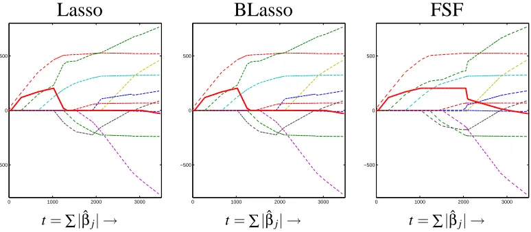
The middle panel of Figure 1 shows the coefficient path plot for BLasso applied to the modified diabetes data. Left (Lasso) and Middle (BLasso) panels are indistinguishable from each other. Both FSF and BLasso pick up the added artificial and strongly correlated X11(the solid line) in the earlier stages, but due to the greedy nature of FSF, it is not able to remove X11in the later stages thus every parameter estimate is affected leading to significantly different solutions from Lasso.
The BLasso solutions were built up in 8700 steps (making the step sizeε=0.5 small so that the coefficient paths are smooth), 840 of which were backward steps. In comparison, FSF took 7300 pure forward steps. BLasso’s backward steps concentrate mainly around the steps where FSF and BLasso tend to differ.
6.2 Comparison of BLasso and Forward Stagewise Fitting by Simulation
Lasso
BLasso
FSF
0 1000 2000 3000
−500 0 500
0 1000 2000 3000
−500 0 500
0 1000 2000 3000
−500 0 500
t=∑|βˆj| → t=∑|βˆj| → t=∑|βˆj| →
Figure 1: Regularization path plots, for the diabetes data set, of Lasso, BLasso and FSF: the curves (or paths) of estimates ˆβj for 10 original and 1 added covariates (predictors), as the
reg-ularization is relaxed or t tends to infinity. The thick solid curves correspond to the 11th added covariate. Left Panel: Lasso solution paths (produced using simplex search method on the penalized empirical loss function for eachλ) as a function of t=kβk1. Middle Panel: BLasso solution paths, which can be seen indistinguishable to the Lasso solutions. Right Panel: FSF solution paths, which are different from Lasso and BLasso.
We first draw 5 covariance matrices Ci, i=1, ..,5 from.95×Di+.05Ip×pwhere Diis sampled
from Wishart(20,p)then normalized to have 1’s on diagonal. The Wishart distribution creates a fair amount of correlation in Ci (average absolute value is about 0.18) between the covariates and
the added identity matrix guarantees Ci to be full rank. For each of the covariance matrix Ci, the
design X is then drawn independently from N(0,Ci)with n=50.
The target variable Y is then computed as
Y =Xβ+e,
whereβ1 toβq with q=7 are drawn independently from N(0,1) andβ8toβ500 are set to zero to create a sparse model. e is the Gaussian noise vector with mean zero and variance 1. For each of the 5 cases with different Ci, both BLasso and FSF are run using stepsizesε=15, 101, 201, 401 and801.
We also run Lasso which is listed as BLasso whenε=0.
To compare the performances, we examine the solutions on the regularization paths that give the smallest mean squared errorkXβ−X ˆβk2. The mean squared error (on log scale) of these solutions are tabulated together with the number of nonzero estimates in each solution. All cases are run 50 times and the average results are reported in Table 1.
Design ε=1 5 ε=
1 10 ε=
1 20 ε=
1 40 ε=
1
80 Lasso (ε=0) C1 MSE BLasso 18.60 18.27 18.33 18.60 19.42 19.98
FSF 19.77 19.40 19.60 19.82 19.96 ˆ
q BLasso 15.38 20.08 21.76 21.44 20.50 21.86 FSF 18.32 24.00 27.28 30.48 32.14
C2 MSE BLasso 19.58 19.28 19.65 19.94 20.76 21.12
FSF 20.67 20.29 20.63 20.94 21.11 ˆ
q BLasso 14.80 18.92 20.18 21.22 20.52 21.82 FSF 18.34 21.90 25.70 28.80 29.38
C3 MSE BLasso 18.83 18.14 18.55 18.90 19.32 20.15
FSF 19.35 19.11 19.52 19.78 19.93 ˆ
q BLasso 15.22 19.10 19.92 20.02 19.52 21.08 FSF 15.38 19.72 23.30 25.88 27.30
C4 MSE BLasso 20.09 19.88 19.85 20.20 21.84 21.70
FSF 21.53 21.09 21.13 21.35 21.57 ˆ
q BLasso 15.76 20.82 22.20 22.42 21.12 22.24 FSF 18.90 24.64 30.38 32.02 34.16
C5 MSE BLasso 18.79 18.62 18.70 19.09 19.47 20.12
FSF 19.99 19.92 19.84 20.19 20.36 ˆ
q BLasso 15.58 19.16 21.26 21.92 22.18 22.76 FSF 17.10 23.24 28.24 30.94 32.84
Table 1: Comparison of FSF and BLasso in a simulated nonparametric regression setting. The log of MSE and ˆq=# of nonzeros are reported for the oracle solutions on the regularization paths. All results are averaged over 50 runs.
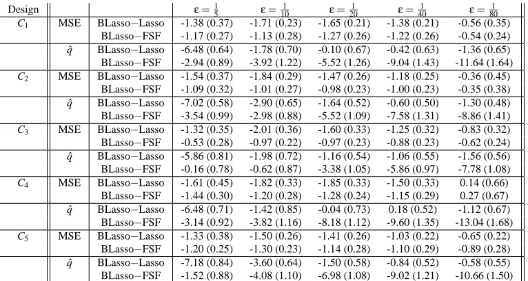
Design ε=1
5 ε=101 ε=201 ε=401 ε=801 C1 MSE BLasso−Lasso -1.38 (0.37) -1.71 (0.23) -1.65 (0.21) -1.38 (0.21) -0.56 (0.35)
BLasso−FSF -1.17 (0.27) -1.13 (0.28) -1.27 (0.26) -1.22 (0.26) -0.54 (0.24) ˆ
q BLasso−Lasso -6.48 (0.64) -1.78 (0.70) -0.10 (0.67) -0.42 (0.63) -1.36 (0.65) BLasso−FSF -2.94 (0.89) -3.92 (1.22) -5.52 (1.26) -9.04 (1.43) -11.64 (1.64)
C2 MSE BLasso−Lasso -1.54 (0.37) -1.84 (0.29) -1.47 (0.26) -1.18 (0.25) -0.36 (0.45)
BLasso−FSF -1.09 (0.32) -1.01 (0.27) -0.98 (0.23) -1.00 (0.23) -0.35 (0.38) ˆ
q BLasso−Lasso -7.02 (0.58) -2.90 (0.65) -1.64 (0.52) -0.60 (0.50) -1.30 (0.48) BLasso−FSF -3.54 (0.99) -2.98 (0.88) -5.52 (1.09) -7.58 (1.31) -8.86 (1.41)
C3 MSE BLasso−Lasso -1.32 (0.35) -2.01 (0.36) -1.60 (0.33) -1.25 (0.32) -0.83 (0.32)
BLasso−FSF -0.53 (0.28) -0.97 (0.22) -0.97 (0.23) -0.88 (0.23) -0.62 (0.24) ˆ
q BLasso−Lasso -5.86 (0.81) -1.98 (0.72) -1.16 (0.54) -1.06 (0.55) -1.56 (0.56) BLasso−FSF -0.16 (0.78) -0.62 (0.87) -3.38 (1.05) -5.86 (0.97) -7.78 (1.08)
C4 MSE BLasso−Lasso -1.61 (0.45) -1.82 (0.33) -1.85 (0.33) -1.50 (0.33) 0.14 (0.66)
BLasso−FSF -1.44 (0.30) -1.20 (0.28) -1.28 (0.24) -1.15 (0.29) 0.27 (0.67) ˆ
q BLasso−Lasso -6.48 (0.71) -1.42 (0.85) -0.04 (0.73) 0.18 (0.52) -1.12 (0.67) BLasso−FSF -3.14 (0.92) -3.82 (1.16) -8.18 (1.12) -9.60 (1.35) -13.04 (1.68)
C5 MSE BLasso−Lasso -1.33 (0.38) -1.50 (0.26) -1.41 (0.26) -1.03 (0.22) -0.65 (0.22)
BLasso−FSF -1.20 (0.25) -1.30 (0.23) -1.14 (0.28) -1.10 (0.29) -0.89 (0.28) ˆ
q BLasso−Lasso -7.18 (0.84) -3.60 (0.64) -1.50 (0.58) -0.84 (0.52) -0.58 (0.55) BLasso−FSF -1.52 (0.88) -4.08 (1.10) -6.98 (1.08) -9.02 (1.21) -10.66 (1.50)
2 4 6 8 10 12 14
0
20
40
60
80
100
BLasso FSF Lasso
2 4 6 8 10 12 14
0
20
40
60
80
100
BLasso FSF Lasso
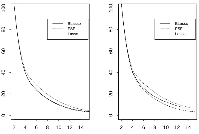
Figure 2: Plots of in-sample Mean Squared Error (y-axis) versuskβk1(x-axis) for a typical realiza-tion of the experiment (on run under C2from Table 1). The step size is set toε= 801 in the left plot andε=1
5 in the right.
As suggested by one referee, we compare the Lasso empirical loss functions induced by BLasso, FSF and Lasso (through LARS). Figure 2 shows plots of in-sample Mean Squared Error versus L1 norms of the coefficients taken from one typical run of the simulation conducted in this section. As shown by the plots, the in-sample MSE from BLasso approximates the in-sample MSE from the Lasso better than the FSF under both big and small step sizes. In particular, when the step size is small, the BLasso path is almost indiscernible from the Lasso path. A final comment on Figure 2 is in order. Although the in-sample MSE curve for BLasso in the right panel of Figure 2 does seem to go up at the end of the plot, we can not extend the x-axis further to higher||β||1 values because at the stepsizeε=1/5, the BLasso solution has achieved its L1norm maximum around 14−15 – the maximum of the x-axis on the right panel of Figure 2.
6.3 Generalized BLasso for Other Penalties and Nondifferentiable Loss Functions
First, to demonstrate Generalized BLasso for different penalties, we use the Bridge Regression setting with the diabetes data set (without the added covariate in the first experiment). The Bridge Regression (first proposed by Frank and Friedman 1993 and later more carefully discussed and implemented by Fu 2001) is a generalization of the ridge regression (L2 penalty) and Lasso (L1 penalty). It considers a linear (L2) regression problem with Lγ penalty forγ≥1 (to maintain the convexity of the penalty function). The penalized loss function has the form:
Γ(β;λ) =
n
∑
i=1
(Yi−Xiβ)2+λkβkγ,
whereγis the bridge parameter. The data used in this experiment are centered and rescaled as in the first experiment.
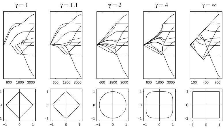
Generalized BLasso successfully produced the paths for all 5 cases which are verified by point-wise minimization using simplex method (γ=1,γ=1.1,γ=4 andγ=max) or close form solutions (γ=2). It is interesting to notice the phase transition from the near-Lasso to the Lasso as the so-lution paths are similar but only Lasso has sparsity. Also, asγgrows larger, estimates for different βj tend to have more similar sizes and in the extremeγ=∞there is a “branching” phenomenon—
the estimates stay together in the beginning and branch out into different directions as the path progresses.
To demonstrate the Generalized BLasso algorithm for classification using an nondifferentiable loss function with a L1penalty function, we look at binary classification with the hinge loss. As in Zhu et al. (2003), we generate n=50 training data points in each of two classes. The first class has two standard normal independent inputs X1 and X2and class label Y =−1. The second class also has two standard normal independent inputs, but conditioned on 4.5≤(X1)2+ (X2)2≤8 and has class label Y=1. We wish to find a classification rule from the training data. so that when given a new input, we can assign a label from{1,−1}to it.
1-norm SVM (Zhu et al., 2003) is used to estimateβ:
(βˆ0,β) =arg min
β0,β n
∑
i=1
(1−Yi(β0+
m
∑
j=1
βjhj(Xi)))++λ
5
∑
j=1
|βj|,
where hi ∈D are basis functions andλ is the regularization parameter. The dictionary of basis
functions is D={√2X1,√2X2,√2X1X2,(X1)2,(X2)2}. Notice thatβ
γ=1 γ=1.1 γ=2 γ=4 γ=∞
600 1800 3000 600 1800 3000 600 1800 3000 600 1800 3000 100 400 700
−1 0 1
−1 0 1
−1 0 1
−1 0 1
−1 0 1
−1 0 1
−1 0 1
−1 0 1
−1 0 1
−1 0 1
Figure 3: Upper Panel: Solution paths produced by BLasso for different bridge parameters, on the diabetes data set. From left to right: Lasso (γ=1), near-Lasso (γ=1.1), Ridge (γ=2), over-Ridge (γ=4), max (γ=∞). The Y -axis is the parameter estimate and has the range [−800,800]. The X -axis for each of the left 4 plots is∑i|βi|, the one for the 5th plot is
max(|βi|) because∑i|βi|is unsuitable. Lower Panel: The corresponding penalty equal
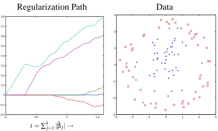
Regularization Path
Data
0 0.5 1 1.5
−0.2 −0.1 0 0.1 0.2 0.3 0.4 0.5 0.6 0.7 0.8
−3 −2 −1 0 1 2 3
−3 −2 −1 0 1 2 3
t=∑5j=1|βˆj| →
Figure 4: Estimates of 1-norm SVM coefficients ˆβj, j=1,2,...,5, for the simulated two-class
classi-fication data. Left Panel: BLasso solutions as a function of t=∑5
j=1|βˆj|. Right Panel:
Scatter plot of the data points with labels: ’+’ for y=−1; ’o’ for y=1.
The fitted model is
ˆ
f(x) =βˆ0+
m
∑
j=1 ˆ βjhj(x),
and the classification rule is given by sign(fˆ(x)).
Since the loss function is not differentiable, we do not have a theoretical guarantee that BLasso works. Nonetheless the solution path produced by Generalized BLasso has the same sparsity and piecewise linearity as the 1-norm SVM solutions shown in Zhu et al. (2003). It takes General-ized BLasso 490 iterations to generate the solutions. The covariates enter the regression equation sequentially as t increase, in the following order: the two quadratic terms first, followed by the interaction term then the two linear terms. As 1-norm SVM in Zhu et al. (2003), BLasso correctly picked up the quadratic terms early. That come up much later are the interaction term and linear terms that are not in the true model. In other words, BLasso results are in good agreement with Zhu et al.’s 1-norm SVM results and we regard this as a confirmation for BLasso’s effectiveness in this nondifferentiable example.
7. Discussion and Concluding Remarks
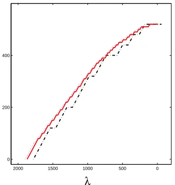
0 500 1000 1500
2000 0 200 400
λ
Figure 5: Estimates of regression coefficients ˆβ3 for the diabetes data set. Solutions are plotted as functions ofλ. Dotted Line: Estimates using stepsizeε=0.05. Solid Line: Estimates using stepsizeε=10. Dash-dot Line: Estimates using stepsizeε=50.
is also effective as an off-the-shelf algorithm for the general convex penalized loss minimization problems.
Computationally, BLasso takes roughly O(1/ε)steps to produce the whole path. Depending on the actual loss function, base learners and minimization method used in each step, the actual compu-tation complexity varies. As shown in the simulations, choosing a smaller stepsize gives a smoother solution path but it does not guarantee a better prediction. Actually, for the particular simulation set-up in Sec. 6.2, moderate stepsizes gave better results both in terms of MSE and sparsity. It is worth noting that the BLasso coefficient estimates are pretty close to the Lasso solutions even for relatively large stepsizes.
For the diabetes data, using a moderate stepsize ε=0.05, the solution path can not be distin-guished from the exact regularization path. Moreover, even when the stepsize is as large asε=10 andε=50, the solutions are still good approximations.
BLasso has only one stepsize parameter (with the exception of the numerical toleranceξwhich is implementation specific but not necessarily a user parameter). This parameter controls both how close BLasso approximates the minimization coefficients for eachλand how close two adjacentλon the regularization path are placed. As can be seen from Figure 5, a smaller stepsize leads to a closer approximation to the solutions and also finer grids forλ. We argue that, ifλis sampled on a coarse grid we should not spend computational power on finding a much more accurate approximation of the coefficients for eachλ. Instead, the available computational power spent on these two coupled tasks should be balanced. BLasso’s 1-parameter setup automatically balances these two aspects of the approximation which is graphically expressed by the staircase shape of the solution paths.
loss function and penalty function and involves calculation of the Hessian matrix which could be heavy-duty computationally when the number p of covariates is not small. In comparison, BLasso uses only the differences of the loss function and involves only basic operations and does not require advanced mathematical knowledge of the loss function or penalty. It can also be used a simple plug-in method for dealplug-ing with other convex penalties. Hence BLasso is easy to program and allows testing of different loss and penalty functions. Admittedly, this ease of implementation can cost computation time in large p situations.
BLasso’s stepsize is defined in the original parameter space which makes the solutions evenly spread inβ’s space rather than inλ. In general, sinceλis approximately the reciprocal of size of the penalty, as a fitted model grows larger andλbecomes smaller, changingλby a fixed amount makes the algorithm in Rosset (2004) move too fast in theβspace. On the other hand, when the model is close to empty and the penalty function is very small,λis very large, but the algorithm still uses the same small steps thus computation is spent to generate solutions that are too close to each other.
As we discussed for the least squares problem, BLasso may also be computationally attractive for dealing with nonparametric learning problems with a large or an infinite number of base learners. This is mainly due to two facts. First, the forward step, as in Boosting, is a sub-optimization problem by itself and Boosting’s functional gradient descend strategy applies. For example, in the case of classification with trees, one can use the classification margin or the logistic loss function as the loss function and use a reweighting procedure to find the appropriate tree at each step (for details see, e.g., Breiman, 1998; Friedman et al., 2000). In the case of regression with the L2 loss function, the minimization as in (6) is equivalent to refitting the residuals as we described in the last section. The second fact is that, when using an iterative procedure like BLasso, we usually stop early to avoid overfitting and to get a sparse model. And even if the algorithm is kept running, it usually reaches a close-to-perfect fit without too many iterations. Therefore, the backward step’s computation complexity is limited because it only involves base learners that are already included from previous steps.
There is, however, a difference in the BLasso algorithm between the case with a small number of base learners and that with a large or an infinite number of base learners. For the finite case, BLasso avoids oscillation by requiring a backward step to be strictly descending and relaxλwhenever no descending step is available. Hence BLasso never reaches the same solution more than once and the tolerance constantξcan be set to 0 or a very small number to accommodate the program’s numerical accuracy. In the nonparametric learning case, a different kind of oscillation can occur when BLasso keeps going back and force in different directions but only improving the penalized loss function by a diminishing amount, therefore a positive toleranceξis mandatory. As suggested by the proof of Theorem 1, we suggest choosingξ=o(ε)to warrant a good approximation to the Lasso path.
One direction for future research is to apply BLasso in an online or time series setting. Since BLasso has both forward and backward steps, we believe that an adaptive online learning algorithm can be devised based BLasso so that it goes back and forth to track the best regularization parameter and the corresponding model.
We end with a summary of our main contributions:
so-lutions for general loss functions and large classes of base learners. This can be proven rigorously for a finite number of base learners under some assumptions.
2. The backward steps introduced in this paper are critical for producing the Lasso path. Without them, the FSF algorithm in general does not produce Lasso solutions, especially when the base learners are strongly correlated as in cases where the number of base learners is larger than the number of observations. As a result, FSF loses some of the sparsity provided by Lasso and might also suffer in prediction performance as suggested by our simulations.
3. We generalized BLasso as a simple, easy-to-implement, plug-in method for approximating the regularization path for other convex penalties.
4. Discussions based on intuition and simulation results are made on the regularization effect of using stepsizes that are not very small.
Last but not least, matlab codes by Guilherme V. Rocha for BLasso in the case of L2loss and L1 penalty can be downloaded at
http://www.stat.berkeley.edu/twiki/Research/YuGroup/Software.
Acknowledgments
Yu would like to gratefully acknowledge the partial supports from NSF grants FD01-12731 and CCR-0106656 and ARO grant DAAD19-01-1-0643, and the Miller Research Professorship in Spring 2004 from the Miller Institute at University of California at Berkeley. We thank Dr. Chris Holmes and Mr. Guilherme V. Rocha for their very helpful comments and discussions on the paper. Fi-nally, we would like to thank three referees and the action editor for their thoughtful and detailed comments on an earlier version of the paper.
Appendix A. Proofs
Proof (Lemma 1)
1. It is assumed that there existλand j with|s|=εsuch that Γ(s1j;λ)≤Γ(0;λ).
Then we have
n
∑
i=1
L(Zi; 0)− n
∑
i=1
L(Zi; s1j)≥λT(s1j)−λT(0).
Therefore
λ ≤ 1ε{ n
∑
i=1
L(Zi; 0)− n
∑
i=1
L(Zi; s1j)}
≤ 1ε{ n
∑
i=1
L(Zi; 0)− min j0,|s|=ε
n
∑
i=1
L(Zi; s1j0)}
= 1
ε{
n
∑
i=1
L(Zi; 0)− n
∑
i=1
L(Zi; ˆβ0)}
2. Since a backward step is only taken when Γ(βˆt+1;λt)<Γ(βˆt;λt)−ξandλt+1=λt, so we
only need to consider forward steps. When a forward step is forced, if Γ(βˆt+1;λt+1)> Γ(βˆt;λt+1)−ξ, then
n
∑
i=1
L(Zi; ˆβt)− n
∑
i=1
L(Zi; ˆβt+1)−ξ<λt+1T(βˆt+1)−λt+1T(βˆt).
Hence
1 ε{
n
∑
i=1
L(Zi; ˆβt)− n
∑
i=1
L(Zi; ˆβt+1)−ξ}<λt+1,
which contradicts the algorithm.
3. Sinceλt+1<λt andλcan not be relaxed by a backward step, we immediately havekβˆt+1k 1=
kβˆtk
1+ε. Then from
λt+1=1 ε{
n
∑
i=1
L(Zi; ˆβt)− n
∑
i=1
L(Zi; ˆβt+1)−ξ},
we get
Γ(βˆt;λt+1)−ξ=Γ(βˆt+1;λt+1). Add(λt−λt+1)kβˆtk
1to both sides, and recall T(βˆt+1) =kβˆt+1k1>|βˆtk1=T(βˆt), we get Γ(βˆt;λt)−ξ < Γ(βˆt+1;λt)
= min
j0,|s|=εΓ( ˆ βt+s1
j0;λt)
≤ Γ(βˆt±ε1j;λt)
for all j.
Proof (Theorem 1)
Theorem 3.1 claims that “the BLasso path converges to the Lasso path uniformly” for∑L(Z;β) that is strongly convex with bounded second derivatives inβ. The strong convexity and bounded second derivatives imply the Hessian w.r.t.βsatisfies
mI∇2
∑
LMI,for positive constants M≥m>0. Using these notations, we will show that for any t s.t.λt+1>λt,
we have
kβˆt−β∗(λt)k
2≤( M
mε+ ξ ε
2 m)
√p, (9)
whereβ∗(λt)∈Rpis the Lasso estimate with a regularization parameterλt.
The proof of (9) relies on the following inequalities for strongly convex functions, some of which can be found in Boyd and Vandenberghe (2004). First, because of the strong convexity, we have
∑
L(Z;β∗(λt))≥∑
L(Z; ˆβt) +∇∑
L(Z; ˆβt)T(β∗(λt)−βˆt) +m 2kβ∗(λt)
The L1penalty function is also convex although not strictly convex nor differentiable at 0, but we have
kβ∗(λt)k1≥ kβˆtk1+δT(β∗(λt)−βˆt)
hold for any p-dimensional vectorδwithδi the i’th entry of sign(βˆt)T for the nonzero entries and |δi| ≤1 otherwise.
Putting both inequalities together, we have
Γ(β∗(λt);λt)≥Γ(βˆt;λt) + (∇
∑
L(Z; ˆβt) +λtδ)T(β∗(λt)−βˆt) +m 2kβ
∗(λt)
−βˆtk22. (10)
Using Equation (10), we can bound the L2distance betweenβ∗(λt)and ˆβt by applying
Cauchy-Schwartz to get
Γ(β∗(λt);λt)≥Γ(βˆt;λt)− k∇
∑
L(Z; ˆβt) +λtδk2kβ∗(λt)−βˆtk2+ m2kβ ∗(λt)
−βˆtk22.
SinceΓ(β∗(λt);λt)≤Γ(βˆt;λt), we have
kβ∗(λt)−βˆtk2≤ 2
mk∇
∑
L(Z; ˆβt) +λ
tδk2. (11)
By statement (3) of Lemma 1, for ˆβtj6=0, we have
∑
L(Z; ˆβt±εsign(βˆtj)1j)±λtε≥
∑
L(Z; ˆβt)−ξ. (12)At the same time, by the bounded Hessian assumption, we have
∑
L(Z; ˆβt±εsign(βˆtj)1j)≤∑
L(Z; ˆβt)±ε∇∑
L(Z; ˆβt)Tsign(βˆtj)1j+M 2ε
2. (13)
Connect these two inequalities, we have
∓ε×(∇
∑
L(Z; ˆβt)T1jsign(βˆtj) +λt)≤
M 2ε
2+ξ, therefore
|(∇
∑
L(Z; ˆβt)T1jsign(βˆtj) +λt)| ≤M 2ε+
ξ
ε. (14)
Similarly, for ˆβtj=0, instead of (12), we have
∑
L(Z; ˆβt±εsign(βˆtj)1j) +λtε≥∑
L(Z; ˆβt)−ξ.Combine with (13), we have
|∇
∑
L(Z; ˆβt)T1j| −λt ≤M 2ε+
ξ ε.
For j such that ˆβtj=0, we chooseδjappropriately and combine with (14) so that the right hand side
of (11) is controlled by√p×m2 ×(M
2ε+
ξ
References
E.L. Allgower and K. Georg. Homotopy methods for approximating several solutions to nonlinear systems of equations. In W. Forster, editor, Numerical solution of highly nonlinear problems, pages 253–270. North-Holland, 1980.
S. Boyd and L. Vandenberghe. Convex Optimization. Cambridge University Press, 2004.
L. Breiman. Arcing classifiers. The Annals of Statistics, 26:801–824, 1998.
P. Buhlmann and B. Yu. Boosting with the l2 loss: regression and classification. Journal of American Statistical Association, 98, 2003.
E. Candes and T. Tao. The danzig selector: Statistical estimation when p is much larger than n. Annals of Statistics (to appear), 2007.
S. Chen and D. Donoho. Basis pursuit. Technical report, Department of Statistics, Stanford Univer-sity, 1994.
N. Cristianini and J. Shawe-Taylor. An introduction to support vector machines and other kernel-based learning methods. Cambridge University Press, 2002.
D. Donoho. For most large undetermined system of linear equatnions the minimal l1-norm near-solution approximates the sparsest near-solution. Communications on Pure and Applied Mathematics, 59(6):797–829, 2006.
D. Donoho, M. Elad, and V. Temlyakov. Stable recovery of sparse overcomplete representations in the presence of noise. IEEE Trans. Information Theory, 52(1):6–18, 2006.
B. Efron, T. Hastie, and R. Tibshirani. Least angle regression. Annals of Statistics, 32:407–499, 2004.
J. Fan and R.Z. Li. Variable selection via nonconcave penalized likelihood and its oracle properties. Journal of American Statistical Association, 96(456):1348–1360, 2001.
I. Frank and J. Friedman. A statistical view od some chemometrics regression tools. Technometrics, 35:109–148, 1993.
Y. Freund. Boosting a weak learning algorithm by majority. Information and Computation, 121: 256–285, 1995.
Y. Freund and R.E. Schapire. Experiments with a new boosting algorithm. In Machine Learning: Proc. Thirteenth International Conference, pages 148–156. Morgan Kauffman, San Francisco, 1996.
J.H. Friedman. Greedy function approximation: a gradient boosting machine. Annal of Statistics, 29:1189–1232, 2001.
W.J. Fu. Penalized regression: The bridge versus the lasso. Journal of Computational and Graphical Statistics, 7(3):397–416, 2001.
J. Gao, H. Suzuki, and B. Yu. Approximate lasso methods for language modeling. Proceedings of the 21st International Conference on Computational Linguistics and 44th Annual Meeting of the ACL, Sydney, pages 225–232, 2006.
T. Gedeon, A. E. Parker, and A. G. Dimitrov. Information distortion and neural coding. Canadian Applied Mathematics Quarterly, 2002.
T. Hastie, Tibshirani, R., and J.H. Friedman. The Elements of Statistical Learning: Data Mining, Inference and Prediction. Springer Verlag, 2001.
T. Hastie, J. Taylor, R. Tibshirani, and G. Walther. Forward stagewise regression and the monotone lasso. Technical report, Department of Statistics, Stanford University, 2006.
K. Knight and W. J. Fu. Asymptotics for lasso-type estimators. Annals of Statistics, 28:1356–1378, 2000.
L. Mason, J. Baxter, P. Bartlett, and M. Frean. Functional gradient techniques for combining hy-potheses. Advance in Large Margin Classifiers, 1999.
N. Meinshausen and P. B ¨uhlmann. High-dimensional graphs and variable selection with the lasso. Annals of Statistics, 34:1436–1462, 2005.
N. Meinshausen and B. Yu. Lasso-type recovery of sparse representations for high-dimensional data. Annals of Statistics (to appear), 2006.
M.R. Osborne, B. Presnell, and B.A. Turlach. A new approach to variable selection in least squares problems. Journal of Numerical Analysis, 20(3):389–403, 2000a.
M.R. Osborne, B. Presnell, and B.A. Turlach. On the lasso and its dual. Journal of Computational and Graphical Statistics, 9(2):319–337, 2000b.
S. Rosset. Tracking curved regularized optimization solution paths. NIPS, 2004.
S. Rosset, J. Zhu, and T. Hastie. Boosting as a regularized path to a maximum margin classifier. Journal of Machine Learning Research, 5:941–973, 2004.
R.E. Schapire. The strength of weak learnability. Journal of Machine Learning, 5(2):1997–2027, 1990.
B. Sch¨olkopf and A. J. Smola. Learning with kernels: support vector machines, regularization, optimization and beyond. MIT Press, 2002.
R. Tibshirani. Regression shrinkage and selection via the lasso. Journal of the Royal Statistical Society, Series B, 58(1):267–288, 1996.
J.A. Tropp. Just relax: Convex programming methods for identifying sparse signals in noise. IEEE Trans. Information Theory, 52(3):1030 –1051, 2006.
V. N. Vapnik. The Nature of Statistical Learning Theory. Springer-Verlag, New York, 1995.
M. J. Wainwright. Sharp thresholds for noisy and high-dimensional recovery of sparsity using`1 -constrained quadratic programming. Technical Report 709, Statistics Department, UC Berkeley, 2006.
C.-H. Zhang and J. Huang. The sparsity and bias of the lasso selection in high dimensional linear regression. Annals of Statistics (to appear), 2006.
T. Zhang. Sequentiall greedy approximation for certain convex optimization problems. IEEE Trans. on Information Theory, 49(3):682–691, 2003.
P. Zhao and B. Yu. On model selection consistency of lasso. Journal of Machine Learning Research, 7 (Nov):2541–2563, 2006.
J. Zhu, S. Rosset, T. Hastie, and R. Tibshirani. 1-norm support vector machines. Advances in Neural Information Processing Systems, 16, 2003.