On
b-bit Min-wise Hashing for Large-scale Regression and
Classification with Sparse Data
Rajen D. Shah [email protected]
Statistical Laboratory University of Cambridge Cambridge, CB3 0WB, UK
Nicolai Meinshausen [email protected]
Seminar f¨ur Statistik ETH Z¨urich
8092 Z¨urich, Switzerland
Editor:Sanjiv Kumar
Abstract
Large-scale regression problems where both the number of variables,p, and the number of observations,n, may be large and in the order of millions or more, are becoming increasingly more common. Typically the data are sparse: only a fraction of a percent of the entries in the design matrix are non-zero. Nevertheless, often the only computationally feasible approach is to perform dimension reduction to obtain a new design matrix with far fewer columns and then work with this compressed data.
b-bit min-wise hashing (Li and K¨onig, 2011; Li et al., 2011) is a promising dimension reduction scheme for sparse matrices which produces a set of random features such that regression on the resulting design matrix approximates a kernel regression with the resem-blance kernel. In this work, we derive bounds on the prediction error of such regressions. For both linear and logistic models, we show that the average prediction error vanishes asymptotically as long asqkβ∗k2
2/n→0, whereqis the average number of non-zero entries in each row of the design matrix andβ∗ is the coefficient of the linear predictor.
We also show that ordinary least squares or ridge regression applied to the reduced data can in fact allow us fit more flexible models. We obtain non-asymptotic prediction error bounds for interaction models and for models where an unknown row normalisation must be applied in order for the signal to be linear in the predictors.
Keywords: large-scale data, min-wise hashing, resemblance kernel, ridge regression, sparse data.
1. Introduction
The modern field of high-dimensional statistics has now developed a powerful range of methods to deal with data sets where the number of variables p may greatly exceed the number of variables n (see B¨uhlmann and van de Geer (2011) for an overview of recent advances). The prototypical example of microarray data, where p may be in the tens of thousands but n is typically not more than a few hundred, has motivated much of this development. Yet not all modern data sets come in this sort of shape and size. The emerging area of ‘large-scale data’ or the more vaguely defined ‘Big Data’ is a response to
c
the increasing prevalence of computationally challenging data sets as arise in text analysis or web-scale prediction tasks, to give two examples. Here both n and p can run into the millions or more, particularly if interactions are considered. In these ‘large p, large n’ regression scenarios, one can imagine situations where ordinary least squares (OLS) has a competitive performance for prediction, but the sheer size of the data renders it infeasible for computational rather than statistical reasons.
An important feature of many large-scale data sets is that they are sparse: the over-whelming majority of entries in the design matrices are exactly zero. This is not to be confused with signal sparsity, a common assumption in the high-dimensional context. In-deed, when the design matrix is sparse, having only a few variables that contribute to the response would make the expected response values of all observations with no non-zero en-tries for the important variables exactly the same; one expects that such a property would not be possessed by many data sets. However, similarly to the way in which many high-dimensional techniques exploit sparsity to improve statistical efficiency, one might hope that sparsity in the data could be leveraged to yield both computational and statistical improvements, and indeed we demonstrate in this work that this can be achieved.
Kernel machines are an important class of machine learning methods for which such large-scale data poses particularly serious computational challenges. For example, standard implementations of kernel ridge regression would have computational complexityO(n3) and a storage cost ofO(n2) whenpis considered fixed; a largepwill increase these computational costs depending on the kernel to be used. There has therefore been a great deal of work on approximating kernel machines by first randomly mapping the n×p design matrix X
to an×dmatrixS withdpsuch that dot products between rows ofS approximate the kernel evaluated on the corresponding rows ofX. Then a regular ridge regression onS will resemble a kernel ridge regression onX, for example.
A remarkably effective way of forming S that is applicable when the design matrix is sparse and binary, is b-bit min-wise hashing (Li and K¨onig, 2011; Li et al., 2011) which is based on an earlier technique called min-wise hashing (Broder et al., 1998; Cohen et al., 2001; Datar and Muthukrishnan, 2002). Here S is constructed such that the dot product between any two rows ofS,sTi sj, can approximate theresemblance orJaccard similarity or
between the corresponding rows ofX, defined as|zi∩zj|/|zi∪zj|wherezi ={k:Xik 6= 0}.
The empirical performance of regression and classification procedures following b-bit min-wise hashing (Li et al., 2011, 2013) is particularly impressive. Existing theory on b -bit min-wise hashing (Li and K¨onig, 2011) has focused on the variance and bias in the approximation of the kernel. However, there remain significant gaps in our theoretical understanding of this important procedure when used to approximate a kernel machine:
(a) What sorts of regression models is the resemblance kernel well-suited for and how does sparsity of the design matrix play a role?
(b) What is the loss in prediction accuracy due to the approximation provided by b-bit min-wise hashing for different sorts of regression procedures?
(c) What is the overall prediction error incurred by different regression methods following
An answer to (c) would be the ultimate goal here, and it would appear that in order to tackle this one must first solve (a) and (b). In this paper, we take a very different approach and aim to answer (c) directly: rather than considering what sorts of functions lie in the reproducing kernel Hilbert space (RKHS) associated with the resemblance kernel and have low RKHS norms, we look at the sorts of signals that can be approximated well by linear combinations of columns of the matrixSconstructed byb-bit min-wise hashing. In this way, we use the random feature expansions provided by b-bit min-wise hashing to understand the predictive properties of the resemblance kernel.
1.1 Our contributions and organisation of the paper
In this paper we derive finite-sample bounds on the expected risk of linear and logistic regression following dimension reduction throughb-bit min-wise hashing under various dif-ferent models. Our results show that the method, and hence also the resemblance kernel, are particularly suited to sparse data.
We describe theb-bit min-wise hashing algorithm in Section 2 and also discuss in greater details the connection to the resemblance kernel. We also introduce a generalisation ofb-bit min-wise hashing applicable to sparse data with real-valued entries motivated by our theory. Perhaps the simplest sorts of signals that we could hope to be able to fit well are linear signals of the form Xβ∗. In Section 3 we first consider how well a linear combination of columns of S can approximate such a signal. We then study a much larger class of signals defined by first scaling the rows ofXin different ways depending on their sparsity and then forming a linear signal from a scaled version ofX. Some form of row normalisation is often performed on the original data as a pre-processing step, but the optimal normalisation to use is seldom known; our theory shows how b-bit min-wise hashing, and hence also the resemblance kernel, is able to automatically discover an appropriate scaling in several settings.
In Section 4.1 we study the performance of ordinary least squares, ridge regression and
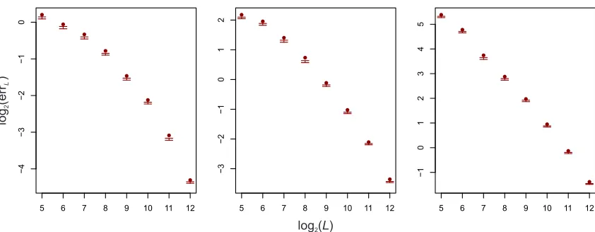
`2-penalised logistic regression using the reduced design matrix it creates. Our results are applicable to both linear signals and nonlinear signals of the sort described above. In the former setting, we show that the expected mean-squared prediction error is bounded by a small constant times pq/nkβ∗k2, where q is the average number nonzero entries in the rows ofXandβ∗ is the coefficient vector. We present similar results for logistic regression. In Section 5 we study another form of nonlinear signal that can be approximated by theb-bit minwise hashing and the resemblance kernel: we show that interaction models in the original data can also be captured by main effects regression on the compressed data. Variable importance measures are discussed in Section 6. We conclude with a discussion in Section 7. The appendix contains all proofs, an additional result concerning the implications of our approximation error bound for properties of the RKHS of the resemblance kernel, and an empirical study validating our bounds.
1.2 Related work
power set of{1, . . . , p}minus the empty set is positive definite. It follows that the RKHS of the resemblance kernel contains every real-valued function onp-dimensional binary vectors (see Section B). However, this result is not informative for understanding which sorts of regression models a kernel ridge regression will perform well for, a question which we provide some answers to through our study ofb-bit min-wise hashing.
Approximating kernel methods using random feature expansions was pioneered by Rahimi and Recht (2007) who used random Fourier features to approximate translation invariant kernels such as the Gaussian kernel. Sutherland and Schneider (2015) provides bounds on the approximation of the corresponding kernel as well as bounds on the distance between the predictions from regression on the random features and kernel ridge regression in terms of distances between the true kernel and its approximation. Le et al. (2013) introduce a scheme related to random Fourier features that further improves the computational effi-ciency. Rahimi and Recht (2008) consider more general random feature expansions and study how well they can approximate functions in a family determined by the distribution of feature expansions in terms of a certain form of function norm defined on the family. Rahimi and Recht (2009) provides prediction error bounds for a method that minimises the empirical risk of a weighted sum of random feature expansions where weights are constrained in`∞-norm. Bach (2017) studies how well random feature expansions can approximate el-ements of their corresponding RKHS in terms of the eigenvalues of the associated kernel integral operator. The Nystr¨om method (Williams and Seeger, 2001) is related and aiming at a computationally efficient low-rank approximation to the full kernel matrix; see (Bach, 2013) and (Rudi et al., 2015) for approximation guarantees.
A distinguishing feature of our work is that bounds are obtained not in terms of the norm of the RKHS of the resemblance kernel, which would be difficult to interpret, but in terms of quantities derived directly from the different models considered (we look at linear models with unknown row scaling and at nonlinear interaction models). We could divide the analysis into two parts: (i) first we could try to understand the predictive accuracy when using exact kernel regression with the resemblance kernel for such true regression functions and then (ii) in a second step understand how much predictive accuracy we lose by using b-bit minwise hashing as an approximation to using exact kernel regression with the resemblance kernel. Instead of making these two separate steps, we study here directly how wellb-bit minwise hashing performs for these model classes.
Properties of b-bit min-wise hashing related to similarity search are studied in Li and K¨onig (2011). Theory concerning its use for large-scale learning is presented in Li et al. (2011) which quantifies the mean and variance of entries in the Gram matrix SST and its relationship to the resemblance kernel as well as providing comparisons with random projections and Vowpal Wabbit. Random feature expansions for other types of kernels are developed in Shi et al. (2009); Weinberger et al. (2009); Vedaldi and Zisserman (2012); Kar and Karnick (2012); Li (2014); Pennington et al. (2015).
dimension reduction at a low computational cost. In this scheme, X is mapped to XA, whereAis ap×dmatrix typically with i.i.d. random entries. Efficient implementations are discussed in Achlioptas (2001); Li et al. (2006) and some numerical results on random pro-jections and a wider literature review are in Fradkin and Madigan (2003); Vempala (2005). The software package Vowpal Wabbit (Langford et al., 2007) is a popular learning system for large-scale data sets that uses sparse random projections.
A separate line of work has considered pre-multiplying X with a random matrix A ∈
Rm×n to produce a reduced matrixAX ∈Rm×p, known as a sketch. Though the
dimen-sion p is not reduced, when n is large, performing OLS on the sketched matrix may be possible despite the computational infeasibility of applying least squares directly to X. A number of works have studied properties sketched least squares (see Boutsidis and Drineas (2009); Drineas et al. (2011); Mahoney (2011); Pilanci and Wainwright (2015) and references therein) whilst Pilanci and Wainwright (2014) propose an iterative variant of this scheme. Yang et al. (2017) considers sketching ideas in the context of kernel ridge regression.
2. b-bit min-wise hashing
Given a sparse design matrixX∈Rn×p, the aim of dimension reduction is to map this to a
compressed matrixS ∈Rn×d, in a way that is computationally efficient and such that the
relevant information in X is preserved in S. Section 2.2 describes the mapping to S under
b-bit min-wise hashing for binary data, as proposed in Li and K¨onig (2011) and Li et al. (2011). The construction may seem unintuitive at first sight, but we will try to shed light on why the scheme works for linear and interaction models throughout the manuscript.
2.1 Notation
Given a matrix U, we will write ui and Uj for the ith row and jth column respectively,
where both are to be regarded as column vectors. The ijth entry will be denoted Uij. A
vector of 1’s will be denoted1.
When the parentheses following probability and expectation signs, P and E, enclose
multiple potential sources of randomness, we will sometimes add subscripts to indicate what is being considered as random. For example, if U and V are random variables, we may writeEU(U|V) for the conditional expectation ofU given V, andEU,V(U+V) for the
expected value ofU +V.
2.2 Construction of S with b-bit min-wise hashing and binary variables
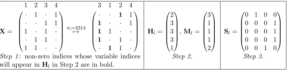
The compressed matrix S generated by b-bit min-wise hashing consists of blocks of size 2b, where we may choose the number of blocks L. Each block is created using a random permutation and the blocks of columns form a collection ofL i.i.d. random matrices.
There are three steps to the construction.
Step 1: Generate a random permutation of the set{1, . . . , p},πl, and permute the columns of X according to this permutation.
the original order) with the first non-zero value or the vector Ml∈Nn the indices of
the variables (indexed as in the permuted order) with the first non-zero value.
Step 3: FormSl∈ {0,1}n×2
b
withith row given by the lastbbits of the binary representation of the ith entry ofMl. For example, whenb= 1, all odd numbers in Ml map to the
vector (0,1), whereas all even numbers map to (1,0).
This construction is illustrated for a toy example in Table 1.
X=
1 2 3 4
· 1 · 1
· · 1 1 1 · 1 · · 1 1 ·
1 1 · ·
πl=2314
7→
3 1 2 4
· · 1 1
1 · · 1
1 1 · ·
1 · 1 ·
· 1 1 ·
Hl= 2 3 3 3 1
,Ml= 3 1 1 1 2 Sl=
0 1 0 0 0 0 0 1 0 0 0 1 0 0 0 1 0 0 1 0
Step 1: non-zero indices whose variable indices will appear inHl in Step 2 are in bold.
Step 2. Step 3.
Table 1: Steps 1–3 applied to a toy example withb= 2. Dots represent zeroes.
We can think of each column of Sl as representing different categories for the
obser-vations. The matrix Sl itself codes for the assignment of the different rows of X to the
different categories. Different blocks Sl then represent different random categorisations.
Identical rows will always be assigned the same categories and the more different the rows are, the less likely they are to be assigned the same category. The notion of difference here is that of resemblance; see Section 2.4
Note that one would not necessarily follow the above steps when implementingb-bit min-wise hashing. In practice, one would not store the entire matrix of signs nor all the random permutations. In an implementation, hash functions (Carter and Wegman, 1979) would be used to create the matrix S deterministically, though it is beyond the scope of this paper to go into the details; see Li et al. (2013) for more information and further computational improvements. With this approach, S would be created row-by-row, and only a single observation fromXwould need to be kept in memory at any one time. Furthermore, many rows could be created in parallel. Other ideas such as one-permutation hashing (Li et al., 2012) can also be used to speed up the pre-processing step.
2.3 Continuous data and additional randomisation
For continuous data, we introduce a modification where we replace the map extracting the last b bits by L random maps in the following way. Fix b and let Ψ ∈ {1, . . . ,2b}p×L be
a random matrix with independent entries each having the uniform distribution on the set
{1, . . . ,2b}. We then create S by modifying the previous Step 3 to the following.
Step 3: FormSl ∈ {0,1}n×2
b
withith row all zero except component ΨHill takes the value 1.
This generalisation is motivated by our theoretical results on how well the column space of S can capture different sorts of signals (see Section 3.1).
Let zi ={k:Xik 6= 0} be the set of variable indices whose entries have non-zero values
for theith observation. Performing the steps above for alll= 1, . . . , L, we getn×Lmatrices
H, and Mgiven by
Hil=arg min k∈zi
πl(k), (1)
Mil= min
k∈ziπl(k) =πl(Hil), (2)
The matrix S is a binaryn×2bL matrix. With a slight abuse of notation, we will denote by Silc thecth entry in the lth block ofS:
Silc:=Si(c+(l−1)2b)=XiHil1{Ψ
Hill=c}, forc= 1, . . . ,2
b. (3)
If not stated otherwise, we will work with this second randomised variation of b-bit min-wise hashing from now on. We emphasise that we do not make the claim this version is to be preferred over the original proposal of Li and K¨onig (2011) and Li et al. (2011) when data is binary. We simply introduce the additional randomisation here to simplify the analysis. We note that the two versions are essentially identical for all practical purposes when bis not too large.
2.4 The resemblance kernel
We now briefly describe the connection betweenb-bit min-wise hashing and the resemblance kernel alluded to earlier. This is not needed for the rest of the paper, though it provides some intuition for the scheme. A more detailed analysis from this perspective is carried out by Li et al. (2011) and we refer the reader to Hofmann et al. (2008) for a review of kernel methods and the kernel trick.
Suppose X is binary. Consider the normalised Gram matrix of the compressed de-sign S from (randomised)b-bit min-wise hashing, SST/L. The expected value of theijth component may be calculated as follows.
Eπ,Ψ(sTi sj/L) =
1
L
L
X
l=1 2b
X
c=1
Eπ,Ψ(1{ΨHill=c}1{ΨHjll=c}) =P(ΨHill = ΨHjll)
=P(ΨHill = ΨHjll|Hil =Hjl)P(Hil=Hjl)
+P(ΨHill = ΨHjll|Hil 6=Hjl){1−P(Hil=Hjl)}
= |zi∩zj|
|zi∪zj|
(1−2−b) + 2−b.
Thus the ijth entry is an average of L i.i.d. random variables with expectation a constant plus a constant times the resemblance between the ith andjth rows of X. If an intercept term is included when regressing onS, the additive constant plays no part, and the scaling would be absorbed into the scaling of the regression coefficients. We also note that when
Now as the resemblance kernel is positive definite, the theory surrounding the kernel trick tells us that any`2-regularised regression onSis effectively approximating a regularised regression on transformed data φ(xi) where φ: {0,1}p → H and H is a high-dimensional
inner product space (the feature space). This space may be taken to be a reproducing kernel Hilbert space (RKHS), and thenφand H are uniquely defined.
Although this is encouraging, the kernel trick does not guarantee that regression on S
will necessarily have good predictive properties for models of interest. To gain a better understanding, we must study the regularisation properties of the resemblance kernel itself: what characterises those elements of the associated RKHS Hthat have low norm and thus will be penalised less?
A direct analysis of the RKHS corresponding to the resemblance kernel in those terms seems challenging. We take a different approach and explicitly construct regression coeffi-cients forS that approximate signals of interest. By showing that particular signals can be approximated well, we are indirectly discovering elements ofH with low RKHS norm (see also Section B for more details).
3. Approximation error
In this section, we present results that bound the expected prediction error when performing regression on the reduced design matrixSin the contexts of the linear and logistic regression models. Note that throughout the rest of the manuscript, byb-bit min-wise hashing we are referring to the randomised variant described in Section 2.3. Letqi be the number of
non-zero entries in theith row ofX, and letδi =qi/p be the row sparsity. We will assume that
the signal we wish to approximate for the ith observation takes the form
κ(δi)xTi β
∗. (4)
Here β∗ ∈Rp is an unknown vector of coefficients and the function κ allows theith linear
predictor to be scaled in a way which depends on the number of non-zero entries in theith row ofX. Some normalisations of special interest include:
(a) κ(δ) constant. This yields standard linear or logistic regression models.
(b) κ(δ)∝δ−1/2. In text analysis with a bag of words representation of documents, rows of
Xare often scaled to have the same`2-norm to help balance situations when documents vary greatly in length (Banerjee et al., 2005). WhenXis binary, this is exactly achieved by takingκ(δ) =p−1/2δ−1/2, soκ(δi) =qi−1/2.
(c) κ(δ)∝δ−1. This leads to a`1-norm scaling as opposed to the`2-norm scaling mentioned above.
Throughout we will assume that X∈[−1,1]n×p, so the entries inX are bounded. This covers the important case of binary design but also allows for real-valued entries.
3.1 Un-scaled signals
We will first consider un-scaled signals whereκ(δ) in (4) is a constant. Non-constant row-scaling is treated in more detail in the Section 3.2. To begin with we will assume that
qi =q ≥1 for alli= 1, . . . , n, a restriction which simplifies the results but highlights some
interesting properties of b-bit min-wise hashing. Unequal row sparsity is treated in detail in the appendix in Section A.4 but a sketch of the results are given just below Theorem 1.
To simplify notation, we first introduce the following norm for β∈Rp,
kβk2b :=kβk22+ (2b−2)
p
X
k=1
kXkk2 2
n β
2
k. (5)
For b = 1, we have of course that kβk2
b = 2kβk22. For larger values of b, the norm is influenced more heavily by the second term which can be seen to be the weighted version of the`2-norm, where the weight of each variable is proportional to its squared `2-norm. We will first discuss how well the original signal can be approximated with the column space of the matrixS generated by theb-bit min-wise hashing operation.
Theorem 1 Let S be the matrix generated byb-bit min-wise hashing. Then there exists a vector b∗∈R2bL with the following properties.
(i) The approximation is unbiased: Eπ,Ψ(Sb∗) =Xβ∗.
(ii) The norm is bounded by
Eπ,Ψ(kb∗k22)≤
(2−δ)q L(1−2−b)kβ
∗k2 2.
(iii) The approximation error is bounded by
1
nEπ,Ψ(kSb
∗−
Xβ∗k22)≤ (2−δ)q
2bL(1−2−b)kβ
∗k2
b.
Specifically, forb= 1,Eπ,Ψ(kSb∗−Xβ∗k22)/n≤(2−δ)qkβ∗k22/L.
A form of the approximation error (iii) and the norm bound (ii) continue to be valid in the non-equal sparsity case under a mild restriction on the size of L, where we get instead of (iii) the bound
1
nEπ,Ψ(kSb
∗−
Xβ∗k22)≤ 6¯q
2bL(1−2−b)kβ
∗k2
b,
where ¯q is the the average of theqi; see Theorem 12 in the appendix for details.
The results above show that the signal Xβ∗ can be well approximated by a linear combination of the columns in the matrix S if we generate a sufficiently large number of permutations L, especially for sparse data matrices. Another useful property of b∗ here, aside from the approximation accuracy it delivers, is given in (ii): on average,kb∗k2
sparsity q, linear functions fβ defined by coefficients β ∈Rp with Pjβj = 0 have RKHS
norm satisfying kfβk2H ≤(2−δ)qkβk22. As these properties of the RKHS are not directly used in any subsequent results, we defer formal presentation of these facts to Section B in the appendix.
Whilst the bound on the expectation of kb∗k2
2 is almost constant as b changes, the ap-proximation error bound (iii) does vary withb. Consider the case whereXis binary and let
γk =kXkk22/nbe the column sparsity. Typically one would expectkβ ∗k2
2 to be significantly larger than Pp
k=1γkβ ∗
k
2 and thus increasing b by 1 almost halves the approximation error when bis small.
A proof of Theorem 1 is given in Section A of the appendix; here we briefly sketch some of the main ideas. Note that
Eπ,Ψ(Sb∗) =
L
X
l=1
Eπ,Ψ
2b X
c=1
Slcb∗lc
. (6)
We construct b∗ with the following two properties: each of the L blocks of b∗ are i.i.d. with the lth block only depending on πl and Ψl; and each of the L summands in (6)
equals Xβ∗/L. With each of the Lsummands being unbiased in this way, we see that the approximation error is controlled by the variance of the sum; this variance scales as 1/L
since the summands are i.i.d.
At first sight it may seem surprising that it is possible to exhibit a b∗ with each block having the unbiasedness property discussed above. However, the following construction gives an indication of the possibilities. Using our convention that thecth component of the
lth block of b∗ is indexed asb∗lc :=b∗c+(l−1)2b, consider taking
b∗lc = q
L
p
X
k=1
βk∗1{Ψlk=c}−2
−b
1−2−b . (7)
Then writingψ =Ψ1,π=π1,Hi =Hi1 we have
L qEπ,ψ
2b X
c=1
Slcb∗1c
=Eπ,ψ
2b X
c=1
p
X
j=1
Xij1{Hi=j,ψj=c}
p
X
k=1
βk∗1{ψk=c}−2
−b
1−2−b
=Eπ,ψ
p X
j=1
Xij1{Hi=j}
p
X
k=1
βk∗1{ψk=ψj}−2
−b
1−2−b
. (8)
Now sinceEψ{(1{ψk=ψj}−2
−b)/(1−2−b)}=1{
k=j} we see the above display equals
q
p
X
k=1
Xikβk∗Pπ(Hi =k) =Xβ∗.
The final line uses the fact that for k with Xik 6= 0, Pπ(Hi = k) is the reciprocal of
sparsity. However as shown in Section A.4, it turns out that by incurring some bias one can still keep the approximation error low even in this situation without having to perform any sort of scaling.
The form of b∗ used in the proof of Theorem 1 differs slightly from that in (7) by introducing a random weight multiplying each coefficient that decays as πl(k) increases.
This reduces the variance and yields the approximation error in (iii) that has a factor q
rather than the factor ofp which would be obtained from (7).
3.2 Row-scaled signals
We now turn to the more general setting with unequal row sparsity and signal given by (4). We consider the family of scaling functions δ 7→ (δmin/δ)a where δmin = miniδi, for
1/2 ≤ a≤1. Including δmin in the scaling functions means that were the row sparsity to be equal, the approximation error here would be of the same form as that considered in Theorems 1. We could alternatively replace δmin with the average of the δi for the same
effect, but using δmin helps to simplify the results. Writing qmin = miniqi, we have the
following results.
Theorem 2 Let L≥5 and assume δmin≤1/2 if a= 1/2, and L >2/(2a−1) if a >1/2.
Then there exists b∗∈RL depending ona such that the approximation error satisfies
1
n
n
X
i=1
Eπ,Ψ[{(δmin/δi)axTi β
∗−
sTi b∗}2]≤
qmin
2bL(1−2−b)kβ
∗k2
blog{4 log(L)/δmin} if a= 1/2,
qmin
2bL(1−2−b)kβ
∗k2
b
1
2a−1[log{2(2a−1)L}]
2a−1 if 1/2< a≤1,
and the norm of b∗ is bounded in expectation by
Eπ,Ψ(kb∗k22)≤
qminlog{4 log(L)/δmin}
L(1−2−b) kβ
∗k2
2 if a= 1/2,
1 2a−1
qmin[log{2(2a−1)L}]2a−1
L(1−2−b) kβ
∗k2
2 if 1/2< a≤1. The min-wise hashing based dimension reduction scheme appears to be well-suited to ap-proximating signals scaled by a power of the sparsity, with the approximation error only incurring a further multiplicative term involving log(L) compared to the results of Theo-rem 1.
We now briefly outline how we construct coefficient vectors b∗ achieving the bounds above. Consider the following refinement of (7):
b∗lc = 1
L
p
X
k=1
βk∗1{Ψlk=c}−2
−b
wherew∈Rp is a vector of non-negative weights. Arguing as in (8) but replacingqβ∗
k with
βk∗wπ(k) we arrive at
LEπ,ψ
2b X
c=1
Slcb∗1c
=
p
X
k=1
Xikβk∗Eπ(1{Hi=k}wπ(k)).
Recall that writingMi =Mi1,Mi =π(Hi), the position of the first non-zero entry in rowi
under permutationπ. Note that Hi and Mi are independent. Now for large p,Mi behaves
roughly like a geometric random variable with parameter δi. Thus fork withXik6= 0,
Eπ(1{Hi=k}wπ(k)) =Eπ(1{Hi=k}wMi)≈
1
pδi p
X
`=1
w`δi(1−δi)`−1 =
1
p
p
X
`=1
w`(1−δi)`−1.
If w`+1 =p(−1)`κ(`)(1)/`! we see that the RHS resembles a Taylor series ofκ(δi) about 1.
In this way we can approximate a large family of row-scaled signals.
4. Prediction error
The approximation error results in the three previous sections allow us to derive bounds on the prediction errors for linear and logistic regression models with potentially row-scaled data. Here we will present results under the assumption ofq non-zero entries per row and also where the scaling functionκ is proportional to the square-root function
κ0(δ) =pδmin/δ. (9)
However, all of the approximation error results can be extended to results on prediction error via general theorems on prediction error we present in Section D. In particular, Theorem 12 can be used to show that versions of the equal row sparsity results hold more generally with
q replaced by the average number of non-zeroes per row ¯q provided L is not excessively large.
4.1 Linear regression models
Assume we have the following approximately linear model:
Yi =α∗+κ(δi)xTi β∗+εi, 1 = 1, . . . , n. (10)
Hereα∗is the intercept andxi ∈[−1,1]p. We assume that the random noiseε∈Rnsatisfies E(εi) = 0,E(εi2) =σ2 and Cov(εi, εj) = 0.
Our results here give bounds on a mean-squared prediction error (MSPE) of the form
MSPE(( ˆα,bˆ)) := 1
n
n
X
i=1
Eε,π,Ψ{(α∗+κ(δi)xTi β
∗−αˆ−Sbˆ)2} (11)
4.1.1 Ordinary least squares
Perhaps the simplest way to estimate the linear model is to apply a least squares estimator,
( ˆα,bˆ) := arg min (α,b)∈R×R2bL
kY−α1−Sbk22, (12) to the matrixS. We have the following theorem.
Theorem 3 Let ( ˆα,bˆ) be the least squares estimator (12). We have the bound
MSPE(( ˆα,bˆ)) ≤ C
2bL(1−2−b) kβ
∗k2
b + 2bL
σ2 n .
For equal row sparsity δ we have C = (2−δ)q. For unequal row sparsity, when κ =κ0 as
in (9), the result holds for C=qminlog{4 log(L)/δmin}.
An optimal choice L∗b of L will balance the approximation error and variance contribu-tions (first and second term on the right hand side respectively). In the equal row sparsity we arrive at
L∗b = p
(2−δ)qn
2b√1−2−bkβ
∗k
b
which yields an optimal MSPE of the order σpq/nkβ∗kb. If we ignore log terms the rate is analogous in the case of uneven row-sparsity. The slow rate in n seems unavoidable if we do not make stronger conditions on the design. Indeed, a similar error rate is obtained in Theorem 21 of Maillard and Munos (2012) and in Kaban (2014) for OLS following dimension reduction by random projections. More precisely: projecting K times with a random projection, followed by an OLS estimation is shown in Kaban (2014) to lead to a bound on MSPE of
1
K kβ
∗k2
κ+K
σ2
n , (13)
where the normk · kκ depends on the eigenvalue structure of the design matrix. In contrast the bound we have above for min-wise hashing depends in contrast on the sparsityqthrough the constant C. The bound (13) is otherwise structurally identical to the bound for b-bit min-wise hashing above, and the role of the number L of projections is now taken by the number K of random projections. The optimal values ofK and L are both of order √n, leading to the same convergence rate of the risk asn→ ∞.
To better understand the implications of Theorem 3, it is helpful to fix the size of the signal so thatkXβ∗k2
2/n= 1, and look at whether we can show consistency of the method as both p, n → ∞. If the signal is spread out and all variables have the same sparsity,
kβ∗kb will be of order pp/qand the MSPE will vanish whenp/n→0, which excludes the high-dimensional setting.
However, now assume that the signal is concentrated on a fixed set of variables. The normkβ∗kb is then constant aspincreases and all that is required for consistency isq/n→0 (orqmin/n→0 for the more general case of uneven row-sparsity).
the first block of predictor variables might encode the presence of individual words. The next block might code for bigrams and the following, higher order N-grams. With this design, predictor variables in each successive block become sparser than the previous. It is then interesting to consider how much the MSPE can increase if we add a block with many sparse variables which contain no additional signal contribution. The result above indicates that the MSPE only increases as √q. Adding a block of several million (sparse) bigrams might thus have the same statistical effect as adding several thousand (denser) unigrams (individual words).
We now comment the optimal choice of Land computational complexity. If we assume fixed kβ∗k2 and n = O(q), which is all that would be required to keep the prediction error bounded asymptotically, then the optimal dimension of the min-wise projection scales as L∗b = O(q), considering b fixed here. This dimension will in general be a substantial reduction over the original dimension of the data,p, and would result in a correspondingly large reduction in the computational cost of regression. Indeed, ridge regression or the LAR algorithm (Efron et al., 2004) applied to X would have complexity O(q2p), and one would expect that the Lasso (Tibshirani, 1996) would have similar computational cost. In contrast, OLS applied to S would only require O(q3) operations, an improvement of q/p. The discussion above considered an optimal choice of L ≈ L∗b. Even if we cannot afford to work with the optimal dimension L∗b for computational reasons, the bound will still be useful for smaller values ofL. The guarantee on prediction accuracy could not be obtained if, for example, simply a random subset ofLpredictors were chosen and the remaining ones discarded.
The dependence of the bound onbis also interesting: a minimum value occurs forb= 1. However, this would imply a larger value ofL∗b. Note the memory requirement for storing
S would be O(nL∗bb) as b bits would be required to store the locations of each of the nL∗b
nonzeroes. We see that with a constraint on nbL or on the number of permutations L, larger values of b are more favourable, particularly with high sparsity, as this would tend to makekβ∗kb not much larger than kβ∗k2. A different perspective on the optimal choice of b based on the variance of inner products of rows ofS is taken in Li and K¨onig (2011), with similar conclusions.
4.1.2 Ridge regression
Instead of using a least-squares estimator on the transformed data matrix S we can also apply ridge regression (Hoerl and Kennard, 1970). For a given λ > 0, the regression coefficients are found by
( ˆαλ,bˆλ) := arg min
(α,b)∈R×RL
kY−αˆ1−Sbk22 such that kbk22≤λ, (14)
The theorem below gives a bound on the MSPE of ( ˆα,bλˆ ).
Theorem 4 There exist regularisation parameters λdepending on β∗ and S such that
MSPE(( ˆαλ,bλˆ )) ≤ σ
s 2C
(1−2−b)nkβ
∗k 2+
C
2bL(1−2−b)kβ
∗k2
b +
Here the value of C is defined as in Theorem 3 byC = (2−δ)q for equal row sparsityδ and
C=qminlog{4 log(L)/δmin} for κ=κ0 and unequal row-sparsity.
The ridge regression result for large L is similar to that for OLS with an optimal L∗b, though there is a small difference: the leading terms are σkβ∗k2
p
q/n and σkβ∗kb
p
q/n
respectively. Ridge regression takes advantage of the fact that not only do we have a b∗
such that Sb∗ and Xβ∗ are close, we also know that there is a b∗ with this property that has low `2-norm. Our bound on the expected squared `2-norm of b∗ ((ii) in Theorem 1) does not depend much on b. In contrast, OLS only makes use of the approximation error result, (iii) in Theorem 1.
Note that whenLis large, regardless of the value ofb, ridge regression onSapproximates a kernel ridge regression using the resemblance kernel (see Section 2.4). The MSPE of a kernel ridge regression with the resemblance kernel should of course not depend on b, and this observation largely agrees with our result.
Another key difference between ridge regression and OLS here is the following: achieving a good prediction error with OLS hinges on a careful choice of L. In contrast, with ridge regression, L can (and should) be chosen very large, from a purely statistical point of view. However, the constraint on the `2-norm of ˆb needs to be chosen carefully with ridge regression, typically by cross-validation. In practice, the number L of dimensions can be chosen as large as possible according to the available computational budget.
4.2 Logistic regression
We give an analogous result to Theorem 4 for classification problems under logistic loss. Letxi∈[−1,1]p and let Y∈ {0,1}n be an associated vector of class labels. We assume the
model
Yi∼Bernoulli(pi); log
pi
1−pi
=κ(δi)xTi β∗, (15)
with theYi independent fori= 1, . . . , n. Note that we have omitted the separate intercept
term for simplicity.
Here we consider a linear classifier constructed by `2-constrained logistic regression. One can obtain a similar result for unconstrained logistic regression based on Lemma 6.6 of B¨uhlmann and van de Geer (2011), but we do not pursue this further here. Define
ˆ
bλ= arg min
b
1
n
n
X
i=1
−YisTi b+ log{1 + exp(sTi b)}
such that kbk22 ≤λ. (16)
LetE(ˆbλ) denote the excess risk of ˆbλ under logistic loss, so
E(ˆbλ) = 1
n
n
X
i=1 h
−pisTi bλˆ + log{1 + exp(sTi bλˆ )}
i
−1
n
n
X
i=1
−piκ(δi)xTi β
∗
+ log{1 + exp(κ(δi)xTi β
∗ )}
.
(17) We can now state the analogous result to Theorem 4.
Theorem 5 Define p˜∈R by
˜
p:= 1
n
n
X
i=1
pi(1−pi)≤
1
Then we have that there exists a λdepending β∗ andS such that
EY,π,Ψ{E(ˆbλ)} ≤
s
2˜pC
(1−2−b)nkβ
∗k 2+
C
2b+2L(1−2−b)kβ
∗k2
b.
Here the value of C is defined as in Theorem 3 byC = (2−δ)q for equal row sparsityδ and
C=qminlog{4 log(L)/δmin} for κ=κ0 and unequal row-sparsity.
The result illustrates that the usefulness ofb-bit min-wise hashing is not limited to regression problems. In fact, most applications of are classification problems (Li and K¨onig, 2011) and our analysis ofb-bit min-wise hashing here gives a theoretical explanation for its performance in these cases.
5. Interaction models
One of the compelling aspects of regression and classification with b-bit min-wise hashing is the fact that a particular form of interactions between variables can be fitted. This does not require any change in the procedure other than a possible increase in L. To be clear, in order to capture interactions with b-bit min-wise hashing, just as in the main effects case, we create a reduced matrix S and then fit a main effects model to S. The dimension of the compressed data, 2bL, can still be substantially smaller than the O(p2) number of coefficients that would need to be estimated if the interactions were modelled in the conventional way, and so the resulting computational advantage can be very large.
Note that in situations where the number of original predictors, p, may be manageable, including interactions explicitly can quickly become computationally infeasible. For exam-ple, if we start with, 105 variables, the two-way interactions number more than a billion. For larger values ofp, even methods such as Random Forest (Breiman, 2001) or Rule Ensembles (Friedman and Popescu, 2008) would suffer similar computational problems.
We now describe a type of interaction model that can be fitted with b-bit min-wise hashing. Let f∗ ∈Rn be given by
fi∗ =
p
X
k=1
Xikθ
∗,(1)
k + p
X
k,k1=1
Xik1{Xik1=0}Θ ∗,(2)
k,k1, i= 1, . . . , n, (19)
where θ∗,(1) ∈Rp is a vector of coefficients for the main effects terms, and Θ∗,(2) ∈ Rp×p
is a matrix of coefficients for interactions whose diagonal entries are zero. As elsewhere in the paper, throughout this section we will assume thatX∈[−1,1]n×p. Note that ifXwere a binary matrix, then (19) parametrises (in fact over-parametrises) all linear combinations of bivariate functions of predictors; that is all possible two-way interactions are included in the model.
5.1 Approximation error
We will assume that the number of non-zero entries in each row of X is q ≥ 1. However, we believe our proof techniques can be extended to the unequal sparsity and unknown row scaling scenario dealt with in Section 3.2. Furthermore, for technical reasons, we assume here that p≥3.
Let Θ∗ collect together θ∗,(1) and Θ∗,(2) and define the following norms analogously to (5):
kΘ∗k:=kθ∗,(1)k2+
2(2−δ)q X
k,k1,k2 Θ
∗,(2)
kk1 Θ ∗,(2)
kk2
1/2
, (20)
kΘ∗kb :=kθ∗,(1)kb+
2(2−δ)q
X
k,k1,k2 Θ
∗,(2)
kk1 Θ ∗,(2)
kk2 +δ(2
b−2) X
k,k1,k2
kXkk22
n
Θ
∗,(2)
kk1 Θ ∗,(2)
kk2
1/2
.
(21)
Theorem 6 Suppose we have exactly q non-zero entries in each row of X. Then there exists a vector b∗∈R2bL
with the following properties:
(i) The approximation is unbiased,Eπ,Ψ(Sb∗) =f∗.
(ii) The `2-norm is bounded by
Eπ,Ψ(kb∗k22)≤
(2−δ)q L(1−2−b)kΘ
∗k2.
(iii) The approximation error is bounded by
Eπ,Ψ(kSb∗−f∗k22)/n≤
(2−δ)q
2bL(1−2−b)kΘ
∗k2
b.
The bound on the approximation error in (iii) is most suited to situations where there are a fixed number of interaction terms, so
X
k,k1,k2 Θ
∗,(2)
kk1 Θ ∗,(2)
kk2
=O(1). (22)
Then we see that the contribution of the interaction terms to the bound on the approxima-tion error is of orderq2. On the other hand, if we are considering a growing number of many small interaction terms, much tighter bounds than that given by (iii) can be obtained. The bounds above show in particular that the form of function given by (19) lies in the RKHS of the resemblance kernel and its RKHS norm is upper bounded by (2−δ)qkΘ∗k2; further details are given in the appendix Section B.
The results for interaction models corresponding to Theorems 3, 4 and 5 now follow.
5.2 Prediction error
5.2.1 Linear regression models
Assume the model (10) and define the MSPE by (11) but in both cases with Xβ∗ now replaced by f∗ (19). As in the previous section, we will assume that X has q non-zero entries in each row. When OLS estimation is used, we have the following result.
Theorem 7 Let ( ˆα,bˆ) be the least squares estimator (12). Then
MSPE(( ˆα,bˆ)) ≤ (2−δ)q
2bL(1−2−b)kΘ
∗k2
b + 2bL
σ2 n.
To interpret the result, consider a situation where there are a fixed number of interaction and main effects of fixed size, so in particular (22) holds. Then treating b as fixed, the optimal L, L∗ = O(pq2n/σ). If n, q and p increase by collecting new data and adding uninformative variables, then in order for the MSPE to vanish asymptotically, we require
q2/n → 0. Compare this to the corresponding requirement of OLS applied to X, that
p2/n → 0. Particularly in situations of increasing variable sparseness, as discussed in Section 4.1.1, this can amount to a large statistical advantage.
The computational gains can be equally great. If, for example,n≈q2, thenL∗ =O(q2). If ridge regression were applied toXaugmented byO(p2) interaction terms, the number of operations required would beO(p2q4); OLS usingShas complexityO(q6). If insteadn≈p2, then regression with explicitly coded interaction terms would have complexityO(p6), whilst with the compressed data this would be reduced toO(p4q2).
As in the main effects case, the ridge regression result is similar.
Theorem 8 Let the ridge regression estimator be given by (14). There existsλ depending onf∗ and S such that we have
MSPE(( ˆα,bˆ)) ≤σ
s
(2−δ)q n(1−2−b)kΘ
∗k+ (2−δ)q 2bL(1−2−b)kΘ
∗k2
b+
σ2
n.
Similarly to Theorem 4 the result here suggests choosing a large L is always better from a statistical point of view. However, for computational reasons, it may not be possible to takeL much larger thanL∗.
5.2.2 Logistic regression
Here we assume the model (15) and define the excess risk by (17), but in both cases with
Xβ∗ replaced byf∗.
Theorem 9 Define p˜∈R as in (18) and the `2-penalised logistic regression estimator as
in (16). Then we have that there exists λsuch that
EY,π,Ψ{E(ˆbλ)} ≤σ
s ˜
p(2−δ)q n(1−2−b)kΘ
∗k+ (2−δ)q
2b+2L(1−2−b)kΘ
∗k2
b.
6. Extensions
We now describe some extensions to the methodology.
6.1 Variable importance
Typically prediction, rather than model selection, is the primary goal in large-scale applica-tions with sparse data, one reason for this being that we cannot expect a very small subset of variables to approximate the signal well when the design matrix is sparse. Nevertheless, it is often illuminating to study the influence of specific variables or look for the variables that have the largest influence on predictions. Indeed, such study is often undertaken fol-lowing applications of Random Forest (Breiman, 2001), where several variable importance measures allow practitioners to better interpret the fits produced.
We now describe how importance measures can be obtained for b-bit min-wise hashing as described in Section 2.3. Let ˆf : Rp → R be the regression function created following
regression onb-bit min-wise hashed data, and let ˆfi:= ˆf(xi). Furthermore, fork= 1, . . . , p,
let ˆf(−k):= ˆf(xi(−k)), wherexi(−k) is equal to xi but with kth component set to zero.
The vector ˆf −ˆf(−k) is the difference in predictions obtained when fitting to X, and those obtained when fitting to X with the kth column set to zero. When the underlying model in X contains only main effects (10) and no structural error is present, we might expect that
ˆ
f−ˆf(−k)≈β∗kXk.
To obtain a measure of variable importance, one could look at the`2-norm of ˆf−ˆf(−k), for example (Breiman, 2001).
The difference in predictions can be computed relatively easily by considering then×2bL
matrix ˜S with entries given by ˜Silc= ˜Si(c+(l−1)2b =XiH˜
il1{ΨHill˜ =c}, where
˜
Hil := arg min k∈zi\Hil
πl(k).
Thus ˜Hil is the variable index in zi whose value under permutation πl is second smallest
among {πl(k) :k∈zi}. Ifzi\Hil=∅, we simply set ˜Sil= 0. Then
ˆ
fi−fˆ(
−k)
i = L
X
l=1
1{Hil=k}
2b
X
c=1
(Silc−S˜ilc)ˆblc. (23)
Note that we only need to store the n×L matrix H and n×2bL matrices S and ˜S to compute the variable importance for all variables; moreover the latter matrices only have at mostnL non-zero entries each.
Interaction effects are not directly visible, but do manifest themselves in the form of a higher variability among {fˆi−fˆ(
−k)
i : xi ≈ x}, for any given value of x, if variable k is
6.2 Other fitting procedures
Here we have only considered OLS, ridge regression and `2-penalised logistic regression as prediction methods after reducing the design matrix. However, it is also conceivable that other fitting procedures could be suitable. In particular, it would be interesting to look at matching pursuit, boosting and the Lasso, for which results in (Tropp, 2004; B¨uhlmann, 2006; Van De Geer, 2008) could be leveraged. Matching pursuit would have the computa-tional advantage that the entire S matrix would not need to be held in memory. Instead, one could create the columns during the fitting process. Such an approach may be useful for problems where the dimension of the hashing-matrix, 2bL, needs to be very large to achieve a desired predictive accuracy.
7. Discussion
In this paper we have derived approximation error bounds forb-bit min-wise hashing. We were able to show that not only does b-bit min-wise hashing take advantage of sparsity in the design matrix computationally, it is also able to exploit this for improved statistical performance. In particular, the MSPE of regression following dimension reduction by b-bit min-wise hashing is of the formpq/nkβ∗k2 if the data follow a linear model with coefficient vectorβ∗ and q is the average number of non-zero variables for an observation. The linear model can then be well-approximated by the low-dimensionalb-bit min-wise hashed data if the norm ofkβ∗k2 is low, as occurs, for example if the signal is approximately replicated in distinct blocks of variables.
In addition, we have shown that more complicated models such as interaction models can be fitted by a regression on the hashed data matrix that contains only main effects. Though a larger dimensionLof the hashed data may be required than when approximating a main effects model, no further changes are needed to the procedure.
These bounds also reveal some of the predictive properties of the resemblance kernel, and provide an insight into the sorts of regression functions that have small norm in its associated RKHS. More generally, we believe that random feature expansions may well be useful as a theoretical tool to understand properties of otherwise intractable kernels. We expect to see more extensions and applications b-bit min-wise hashing and other random feature expansions, both as computational and theoretical tools, in the future.
Acknowledgments
The first author was supported by The Alan Turing Institute under the EPSRC grant EP/N510129/1 and an EPSRC programme grant.
Appendix A. Approximation error results
A.1 Preliminary results
We will let qi be the number of non-zeroes in the ith row of X and define δi =qi/p. We
will assume thatqi ≥1 for alli. For the proofs of results on approximation error in settings
with just main effects, we will make use of the following lemma. This lemma formalises the ideas of the discussion at the end of Section 3.2, that the elements ofMbehave rather like geometric random variables.
Lemma 10 There exist random functions {gl(k)}l=1,...,L, k=1,...,p defined on the same prob-ability space as the permutations π with the following properties:
(i) The random variables{g1(k)}k=1,...,p, . . . ,{gL(k)}k=1,...,pare i.i.d. and are independent of Ψ.
(ii) The rank of gl(k) among gl(1), . . . , gl(p) taken in increasing order isπl(k).
(iii) Marginallygl(k)∼Geo(p−1).
(iv) Gil := mink∈zigl(k) =gl(Hil)∼Geo(δi).
(v) G and Hare independent.
Proof First consider generating permutations π in the following way. Letm ∈N and let σ1(m), . . . , σ(Lm) be Li.i.d. random permutations of{1, . . . , mp}. Fork= 1, . . . , p, let
gl(m)(k) = min
a=0,...,m−1σ (m)
l (k+ap).
Note that the gl(m)(k) are all distinct and any ordering of them is equally likely so they define a random permutation of{1, . . . , p}. Furthermore, for j= 1, . . . , mp−m+ 1,
P(gl(m)(k) =j) =
mp−j
m−1
mp m
= 1
p
1−1−m
−1
p−m−1
· · ·
1− 1−m
−1
p−(j−1)m−1
.
Thus
P(gl(m)(k) =j)→ 1 p
1−1
p
j−1
as m → ∞ forj = 1,2, . . .. Similarly G(ilm) := mink∈zig(lm)(k) has P(G
(m)
il =j) → δi(1−
δi)j−1 asm→ ∞. Note that G(m) and Hare independent. Thus
{g(lm)(k)}l=1,...,L,k=1,...,p → {d gl(k)}l=1,...,L,k=1,...,p
asm→ ∞with the random variablesgl(k) having the properties given in the statement of
the lemma.
In the proofs which follow, we will consider the permutations as having been generated as described by Lemma 10. We will letπ =π1,Mi =Mi1,g=g1,G1 =Gi1,Hi=Hi1 and
ψ =Ψ1. LetC= 2b,ν= 2−b.
Lemma 11 For a given sequence of weights{wj}∞j=1, letb˜∗ ∈RLC be given by
˜
b∗lc = 1
L
p
X
k=1
βk∗1{Ψlk=c}−ν
1−ν wgl(k)
and let b∗ =E(˜b∗|π). We have the following.
(i)
Eπ,Ψ(sTi b∗) =
1
px
T i β∗
∞ X
`=1
(1−δi)`−1w`.
(ii)
Eπ,Ψ(kb∗k22)≤ 1
pL(1−ν)kβ ∗k2
2 ∞ X
`=1
w2`. (24)
(iii)
Varπ,Ψ(sTi b
∗
)≤ 1
pL(1−ν)
νkβ∗k22+ (1−2ν)
p
X
k=1
Xik2β∗k2
∞ X
`=1
w`2. (25)
Proof First note that
E
1{
ψk=ψj}−ν
1−ν
ψj = (
1 ifk=j
0 otherwise (26)
E
1{
ψk=ψj}−ν
1−ν
1{ψ`=ψj}−ν
1−ν
ψj =
1 ifk=`=j
0 ifk6=`
ν
1−ν otherwise.
(27)
For (i), we have
Eπ,Ψ(sTi b∗) =Eg,ψ
C X c=1 p X j=1
Xij1{Hi=j}1{ψj=c}
p
X
k=1
βk∗1{ψk=c}−ν
1−ν wg(k)
=Eg
p X
k=1
Xik1{Hi=k}β
∗
kwg(k) = 1 qi p X k=1
Xikβk∗E(wGi),
where to arrive at the second line we used (26).
Turning to (ii), note that each component ofb∗ has mean zero and so
E(b∗lc
2
Now we have
Eg1,...,gL,Ψkb˜
∗k2 2= 1 L C X c=1 X k,`
βk∗β`∗E
1{
ψk=c}−ν
1−ν
1{ψ`=c}−ν
1−ν
E(wg(k)wg(`)) Using (27), we get
Eg1,...,gL,Ψkb˜
∗k2 2 =
1
L(1−ν) X
k
βk∗2E(wg2(k))≤ 1
pL(1−ν)kβ ∗k2
2 ∞ X
`=1
w`2.
For (iii) we argue as follows.
Var(sTi b∗)≤Var(sTi b˜∗)
≤ 1
LEg,ψ
XiH2 iX
k,`
βk∗β`∗1{ψk=ψHi}
−ν
1−ν
1{ψ`=ψHi}−ν
1−ν wg(k)wg(`)
Using (27) and the fact thatX∈[−1,1]n×p, we have
Var(sTib∗)≤ 1
LE
XiH2 i
ν
1−ν
p
X
k=1
(βk∗)2wg2(k)+1−2ν 1−ν (β
∗
Hi)
2w2
Gi
(28)
≤ 1
L(1−ν)
ν
p
X
k=1
βk∗2E(w2g(k)) + 1−2ν
qi E
(wG2i)
p
X
k=1
Xik2βk∗2
.
The result then follows as ∞
X
`=1
w`2 ≥E(w2g(k)) = 1 p
∞ X
`=1
w2`
1−1
p
`−1
≥ δi
qi
∞ X
`=1
w2`(1−δi)`−1 =
E(w2Gi) qi
.
A.2 Proof of Theorem 1
We use a b∗ and ˜b∗ as in Lemma 11 but here we choose the weights w` so as to minimise
P∞
`=1w2` (a term which features in our upper bounds on the variance andE(kb
∗k2
2)) subject to the unbiasedness constraint (i). The unbiasedness constraint amounts to
∞ X
`=1
(1−δ)`−1w`=p.
Performing the minimisation with this constraint yields
w` =p
(1−δ)`−1 P∞
`=1(1−δ)2`−2
.
With this choice we have ∞
X
`=1
w2` =p2
∞ X
`=1
(1−δ)2`−2 −1
=p2{1−(1−δ)2}= (2−δ)qp.
A.3 Proof of Theorem 2
We use ab∗ and ˜b∗ as in Lemma 11 but here we take
w`+1 =p(−1)`
κ(`)(1)
`! {1{`≤bmc}+ (m− bmc)1{`=dme}}
wherem >0 is a parameter to be chosen. Thus the weights correspond to coefficients from a truncated Taylor series expansion ofκ about 1. We have
Eπ,Ψ[{(δmin/δi)axTi β
∗−
sTi b∗}2] ={(δmin/δi)axTi β
∗−
Eπ,Ψ(sTi b
∗
)}2+ Varπ,Ψ(sTi b
∗ ).
We first bound the variance term by bounding the squared sum of the sequence of weights. To this end, we note that by Lemma 20
δ−min2a p2
∞ X
`=1
w`2 ≤1 +a2+a2e2a
bmc X
`=2 1
`2(1−a) +
m− bmc dme2(1−a)
.
Now
bmc X
`=2 1
`2(1−a) +
m− bmc dme2(1−a) ≤
Z m
1 1
`2(a−1)d` =
(m2a−1−1
2a−1 ifa6= 1/2 log(m) ifa= 1/2.
Let
τa(m) =
(
elog(me5/e)/4 ifa= 1/2,
a2e2am2a−1/(2a−1) if 1/2< a≤1.
Then
∞ X
`=1
w`2 ≤p2δmin2a τa(m). (29)
The variance is then at most
δmin2a τa(m)
p L(1−ν)
νkβ∗k22+ (1−2ν)
p
X
k=1
Xik2β∗k2
.
Turning now to the bias term, note first that by (i) of Lemma 11, this is equal to
(xTiβ∗)2
(δmin/δi)a−
1
p
∞ X
`=1
(1−δi)`−1w`
2
. (30)
We see this is bounded above by
δ2mina (xTi β∗)2
aea
∞
X
`=dme
(1−δi)`
1
`1−a
2
Now
∞ X
`=dme
(1−δi)`
1
`1−a ≤
e−δim m1−aδ i
.
By the Cauchy–Schwarz inequality (assuming Xij ∈[−1,1])
(xTiβ∗)2
δi
= 1
δi
X
k∈zi Xikβk∗
2
≤p
p
X
k=1
Xik2βk∗2 ≤pkβ∗k22.
Thus the squared bias is at most
p
1−ν a2e2a
m1−2ai=1max,...,n
e−2δim mδi
νkβ∗k22+ (1−2ν)
p
X
k=1
Xik2βk∗2
.
Therefore the MSE (now averaging over the observations) is bounded by the minimum over
m >0 of
p L(1−2−b)δ
2a
min
τa(m) +
a2e2a
m1−2ai=1max,...,n
e−2δim mδi
kβ∗k2
b.
Fora= 1/2, we set m= log(L)/{2δmin}. This yields min
m>0
τ1/2(m) + Le 4 i=1max,...,n
e−2δim mδi ≤ e 4 log
log(L)e5/e
2δmin
+ 2 log(L)
≤log{4 log(L)/δmin}
providedL≥10 and δmin ≤1/2. Finally the bound for a >1/2 comes from setting
m= 1
2log{2(2a−1)L}/δmin which gives
min
m>0
τa(m) +
La2e2a m1−2a i=1max,...,n
e−2δim mδi
≤ δ
1−2a
min a2e2a
22a−1(2a−1)[log{2(2a−1)L}]
2a−2log{2(2a−1)eL}
≤ 4δ
1−2a
min
1−2a[log{2(2a−1)L}]
2a−1
for L ≥2/(1−2a). Using the bounds on τa with these choices of m and (29), we obtain
the bounds on E(kb∗k22) by substituting into (24).
A.4 Unequal row sparsity and constant row-scaling
Here we prove results indicated after the presentation of Theorem 1 in Section 3.1. When the scaling function is simply the constant 1, the spread of theδi becomes more critical in
determining how well the signal can be approximated. Define
¯
δ = 1
n
n
X
i=1
δi,
V(δ) = 1
kXβ∗k2 2
n
X
i=1
Theorem 12 Suppose
2bL(1−2−b)≤ p(2¯δ)
3kβ∗k2
b
kXβ∗k2
2V(δ)/n
. (31)
Then there exists b∗∈RL such that the approximation error satisfies
1
nEπ,Ψ{kXβ
∗−Sb∗k2 2} ≤
6pδ¯
2bL(1−2−b)kβ
∗k2
b, (32)
and
Eπ,Ψ(kb∗k22)≤
2¯q L(1−2−b)kβ
∗k2
2. (33)
Provided 2bL is not too large, we recover essentially the same approximation error bound as Theorem 1 up to a constant factor, but with the row sparsity replaced by the average row sparsity ¯δ. In the simple situation where the entries of X are realisations of i.i.d. Bernoulli random variables with probability δ, we would have ¯δ ≈δ, kXβ∗k2
2/n≈δkβ ∗k2
2 and V(δ) ≈ δ/p. Substituting these values into the requirement on 2bL shows that the condition reduces to 2bL≤8p2δ{1 + (2b−2)δ}. Note that typically one would choose 2bL
of the order ¯δp. More generally, providedV(δ) and kXβ∗k2 2/kβ
∗k2
2 are small, we can expect that the bound of Theorem 1 will hold true, up to a constant factor.
Proof of Theorem 12
We use ab∗ and ˜b∗ as in Lemma 11 taking
w`=p(1−δ¯)`−11{`≤m} ¯
δ(2−δ¯) 1−(1−δ¯)2m.
wherem∈Nis a parameter to be chosen. This gives
1
p2 ∞ X
`=1
w`2 = δ¯(2−δ¯) 1−(1−δ¯)2m,
which gives us a bound on the variance term.
Lemma 11 (i) gives the expression for the bias term. To bound this, first note that
1
p
m
X
`=1
(1−δ¯)`−1w` = 1.
Next
m X
`=1
(1−¯δ)`−1{(1−¯δ)`−1−(1−δi)`−1}
2
= (δi−δ¯)2
m X
`=1
(1−δ¯)`−1
`−2 X
k=0
(1−δ¯)k(1−δi)`−2−k
2
≤(δi−δ¯)2
m X
`=1
(1−δ¯)`−1(`−1) 2
= min
m(m−1) 2 ,
1 ¯
δ2 2
Also note that as
(1−δ¯)2m≤1−2mδ¯+m(2m−1)¯δ2
we have
¯
δ(2−δ¯) 1−(1−δ¯)2m ≤
2
2m−m(2m−1)¯δ1{m≤1/(2¯δ)}+
2
1/δ¯−(1/δ¯−1)/21{m>1/(2¯δ)}
≤max
2
m+ 1/2, 4¯δ
1 + ¯δ
and for m≤1/(2¯δ) + 1/2,
m(m−1) 2 max
2
m+ 1/2, 4¯δ
1 + ¯δ
≤(m−1/2)1{1<m≤1/(2¯δ)+1/2}.
Thus the overall approximation error is bounded above by the minimum overm= 1,2, . . . ,
1/(2¯δ) + 1/2 of
1{m>1}(m−1/2)2 1
nkXβ
∗k2
2V(δ) + max
2
m+ 1/2,4¯δ
p
2bL(1−2−b)kβ
∗k2
b,
which in turn is bounded by the minimum over m∈[0,1/(2¯δ)] of
m21 nkXβ
∗k2
2V(δ) + 2
m
p
2bL(1−2−b)kβ
∗k2
b. (34)
Optimising over m >0 in the above then gives
m= min
pkβ∗k2
b
2bL(1−2−b)kXβ∗k2
2V(δ)/n 1/3
, 1
2¯δ
.
The condition onL(31) ensures that the minimum is achieved at 1/(2¯δ). Substituting this value of m into (34) then gives (32). For (33) we note that
∞ X
`=1
w`2≤2p2δ¯;
the result follows using Lemma 11 (ii).
A.5 Proof of Theorem 6
We let b∗ = b∗,(1) +b∗,(2) where b∗,(1) is chosen in line with Theorem 1. Explicitly, let
b∗,(1) =E(˜b∗|π) where
˜b∗
lc =
p L
p
X
k=1
θk∗,(1)1{Ψlk=c}−ν
1−ν
(1−δ)gl(k)−1
P∞
`=1(1−δ)2`−2
.
We constructb∗,(2) to approximate the interactions as follows. Let
b∗lc,(2) = pq
L
p
X
k=1
1{Ψlk=c}−ν
1−ν
p
X
k1=1 Θ∗kk,(2)
wherew∈Rp is a vector of weights to be chosen such that
Eπ,Ψ(sTi b∗,(2)) =
X
k,k1
Xik1{Xik1=0}Θ
∗,(2)
kk1 . (35)
We compute
Eπ,Ψ(sTib
∗,(2)) = pq
L L X l=1 C X c=1
Eπl,Ψl
Silc p
X
k=1
1{Ψkl=c}−ν
1−ν
p
X
k1=1 Θ∗kk,(2)
1 1{πl(k1)<πl(k)}wπl(k)
=pqEπ,ψ
C X c=1 p X j=1
Xij1{Hi=j}1{ψj=c}
p
X
k=1
1{ψk=c}−ν
1−ν
p
X
k1=1 Θ∗kk,(2)
1 1{π(k1)<π(k)}wπ(k)
=pqEπ
p
X
k=1
Xik1{Hi=k}
p
X
k1=1 Θ∗kk,(2)
1 1{π(k1)<π(k)}
p
X
`=2
w`1{π(k)=`}
.
where in the final line we have appealed to (26). Now observe that fork∈zi,
1{Hi=k}1{π(k1)<π(k)}1{π(k)=`}=1{Xik1=0}1{Hi=k}1{Mi=`, π(k1)<`},
and 1{Hi=k} and1{Mi=`, π(k1)<`} are independent. Thus we have
Eπ,Ψ((Sb∗,(2))i) =
X
k,k1
Xik1{Xik1=0}Θ ∗,(2)
kk1
p
X
`=1
pPπ(Mi=`, π(k1)< `)w`
=X
k,k1
Xik1{Xik1=0}Θ ∗,(2)
kk1
p
X
`=2
(`−1)Pπ(Mi=`|π(k1)< `)w`
=X
k,k1
Xik1{Xik1=0}Θ ∗,(2)
kk1
p
X
`=2 (`−1)
p−` q−1
p−1
q
w`.
Thus if we choosew such that
p
X
`=2 (`−1)
p−` q−1
p−1
q
w`= 1, (36)