Consistent Algorithms for Clustering Time Series
Azadeh Khaleghi [email protected]
Department of Mathematics & Statistics Lancaster University, Lancaster, LA1 4YF, UK
Daniil Ryabko [email protected]
INRIA Lille
40, avenue de Halley
59650 Villeneuve d’Ascq, France
J´er´emie Mary [email protected]
Philippe Preux [email protected]
Universit´e de Lille/CRIStAL (UMR CNRS) 40, avenue de Halley
59650 Villeneuve d’Ascq, France
Editor:G´abor Lugosi
Abstract
The problem of clustering is considered for the case where every point is a time series. The time series are either given in one batch (offline setting), or they are allowed to grow with time and new time series can be added along the way (online setting). We propose a natural notion of consistency for this problem, and show that there are simple, com-putationally efficient algorithms that are asymptotically consistent under extremely weak assumptions on the distributions that generate the data. The notion of consistency is as follows. A clustering algorithm is called consistent if it places two time series into the same cluster if and only if the distribution that generates them is the same. In the considered framework the time series are allowed to be highly dependent, and the dependence can have arbitrary form. If the number of clusters is known, the only assumption we make is that the (marginal) distribution of each time series is stationary ergodic. No paramet-ric, memory or mixing assumptions are made. When the number of clusters is unknown, stronger assumptions are provably necessary, but it is still possible to devise nonparametric algorithms that are consistent under very general conditions. The theoretical findings of this work are illustrated with experiments on both synthetic and real data.
Keywords: clustering, time series, ergodicity, unsupervised learning
1. Introduction
The intuitively appealing problem of clustering is notoriously difficult to formalise. An intrinsic part of the problem is a similarity measure: the points in each cluster are supposed to be close to each other in some sense. While it is clear that the problem of finding the appropriate similarity measure is inseparable from the problem of achieving the clustering objectives, in the available formulations of the problem it is usually assumed that the similarity measure is given: it is either some fixed metric, or just a matrix of similarities between the points. Even with this simplification, it is still unclear how to define good clustering. Thus, Kleinberg (2002) presents a set of fairly natural properties that a good clustering function should have, and further demonstrate that there is no clustering function that satisfies these properties. A common approach is therefore to fix not only the similarity measure, but also some specific objective function — typically, along with the number of clusters — and to construct algorithms that maximise this objective. However, even this approach has some fundamental difficulties, albeit of a different, this time computational, nature: already in the case where the number of clusters is known, and the distance between the points is set to be the Euclidean distance, optimising some fairly natural objectives (such ask-means) turns out to be NP hard (Mahajan et al., 2009).
In this paper we consider a subset of the clustering problem, namely, clustering time series. That is, we consider the case where each data point is a sample drawn from some (unknown) time-series distribution. At first glance this does not appear to be a simplifica-tion (indeed, any data point can be considered as a time series of length 1). However, note that time series present a different dimension of asymptotic: with respect to their length, rather than with respect to the total number of points to be clustered. “Learning” along this dimension turns out to be easy to define, and allows for the construction of consistent algorithms under most general assumptions. Specifically, the assumption that each time series is generated by a stationary ergodic distribution is already sufficient to estimate any finite-dimensional characteristic of the distribution with arbitrary precision, provided the series is long enough. Thus, in contrast to the general clustering setup, in the time-series case it is possible to “learn” the distribution that generates each given data point. No assumptions on the dependence between time series are necessary for this. The assumption that a given time series is stationary ergodic is one of the most general assumptions used in statistics; in particular, it allows for arbitrary long-range serial dependence, and sub-sumes most of the nonparametric as well as modelling assumptions used in the literature on clustering time series, such as i.i.d., (hidden) Markov, or mixing time series.
This allows us to define the following clustering objective: group a pair of time series into the same cluster if and only if the distribution that generates them is the same.
1.1 Problem Setup
We consider two variants of the clustering problem in this setting: offline (batch) and online, defined as follows.
In the offline (batch) setting a finite number N of sequences x1 = (X11, . . . , Xn11), . . . ,xN = (X1N, . . . , XnNN) is given. Each sequence is generated by one of κ different
un-knowntime-series distributions. The target clustering is the partitioning ofx1, . . . ,xN into
κclusters, putting together those and only those sequences that were generated by the same time-series distribution. We call a batch clustering algorithm asymptotically consistent if, with probability 1, it stabilises on the target clustering in the limit as the lengthsn1, . . . , nN
of each of the N samples tend to infinity. The number κ of clusters may be either known or unknown. Note that the asymptotic is not with respect to the number of sequences, but with respect to the individual sequence lengths.
In the online setting we have a growing body of sequences of data. The number of se-quences as well as the sese-quences themselves grow with time. The manner of this evolution can be arbitrary; we only require that the length of each individual sequence tend to infin-ity. Similarly to the batch setting, the joint distribution generating the data is unknown. At time step 1 initial segments of some of the first sequences are available to the learner. At each subsequent time step, new data are revealed, either as an extension of a previ-ously observed sequence, or as a new sequence. Thus, at each time step t a total of N(t) sequences x1, . . . ,xN(t) are to be clustered, where each sequence xi is of length ni(t) ∈N for i = 1..N(t). The total number of observed sequences N(t) as well as the individual sequence lengthsni(t) grow with time. In the online setting, a clustering algorithm is called
asymptotically consistent, if almost surely for each fixed batch of sequences x1, . . . ,xN,
the clustering restricted to this sequences coincides with the target clustering from some time on.
At first glance it may seem that one can use the offline algorithm in the online setting by simply applying it to the entire data observed at every time step. However, this naive approach does not result in a consistent algorithm. The main challenge in the online setting can be identified with what we regard as “bad” sequences: sequences for which sufficient information has not yet been collected, and thus cannot be distinguished based on the pro-cess distributions that generate them. In this setting, using a batch algorithm at every time step results in not only mis-clustering such “bad” sequences, but also in clustering incor-rectly those for which sufficient data are already available. That is, such “bad” sequences can render the entire batch clustering useless, leading the algorithm to incorrectly cluster even the “good” sequences. Since new sequences may arrive in an uncontrollable (even data-dependent, adversarial) fashion, any batch algorithm will fail in this scenario.
1.2 Results
The first result of this work is a formal definition of the problem of time-series clustering which is rather intuitive, and at the same time allows for the construction of efficient algorithms that are provably consistent under the most general assumptions. The second result is the construction of such algorithms.
distribution generating each sequence is stationary ergodic. No restrictions are placed on the dependence between the sequences: this dependence may be arbitrary (and can be thought of as adversarial). This consistency result is established in each of the two settings (offline and online) introduced above.
As follows from the theoretical impossibility results of Ryabko (2010c) that are discussed further in Section 1.4, under the only assumption that the distributions generating the sequences are stationary ergodic, it is impossible to find the correct number of clusters κ, that is, the total number of different time-series distributions that generate the data. Moreover, non-asymptotic results (finite-time bounds on the probability of error) are also provably impossible to obtain in this setting, since this is already the case for the problem of estimating the probability of any finite-time event (Shields, 1996).
Finding the number κ of clusters, as well as obtaining non-asymptotic performance guarantees, is possible under additional conditions on the distributions. In particular, we show that if κ is unknown, it is possible to construct consistent algorithms provided that the distributions are mixing and bounds on the mixing rates are available.
However, the main focus of this paper remains on the general framework where no additional assumptions on the unknown process distributions are made (other than that they are stationary ergodic). As such, the main theoretical and experimental results concern the case of knownκ.
Finally, we show that our methods can be implemented efficiently: they are at most quadratic in each of their arguments, and are linear (up to log terms) in some formulations. To test the empirical performance of our algorithms we evaluated them on both synthetic and real data. To reflect the generality of the suggested framework in the experimental setup, we had our synthetic data generated by stationary ergodic process distributions that do not belong to any “simpler” class of distributions, and in particular cannot be modelled as hidden Markov processes with countable sets of states. In the batch setting, the error rates of both methods go to zero with sequence length. In the online setting with new samples arriving at every time step, the error rate of the offline algorithm remains consistently high, whereas that of the online algorithm converges to zero. This demonstrates that, unlike the offline algorithm, the online algorithm is robust to “bad” sequences. To demonstrate the applicability of our work to real-world scenarios, we chose the problem of clustering motion-capture sequences of human locomotion. This application area has also been studied in the works (Li and Prakash, 2011) and (Jebara et al., 2007) that (to the best of our knowledge) constitute the state-of-the-art performance1 on the data sets they consider, and against which we compare the performance of our methods. We obtained consistently better performance on the data sets involving motion that can be considered ergodic (walking, running), and competitive performance on those involving non-ergodic motions (single jumps).
1.3 Methodology and Algorithms
A crucial point of any clustering method is the similarity measure. Since the objective in our formulation is to cluster time series based on the distributions that generate them, the similarity measure must reflect the difference between the underlying distributions. As we aim to make as few assumptions as possible on the distributions that generate the data, and since we make no assumptions on the nature of differences between the distributions, the distance should take into account all possible differences between time-series distributions. Moreover, it should be possible to construct estimates of this distance that are consistent for arbitrary stationary ergodic distributions.
It turns out that a suitable distance for this purpose is the so-called distributional dis-tance. The distributional distance d(ρ1, ρ2) between a pair of process distributions ρ1, ρ2 is defined (Gray, 1988) as P
j∈Nwj|ρ1(Bj)−ρ2(Bj)|where, wj are positive summable real
weights, e.g. wj = 1/j(j+ 1), and Bj range over a countable field that generates the σ
-algebra of the underlying probability space. For example, consider finite-alphabet processes with the binary alphabet X = {0,1}. In this case Bj, j ∈ N would range over the set X∗ = ∪m∈NXm; that is, over all tuples 0,1,00,01,10,11,000,001, . . .; therefore, the
dis-tributional distance in this case is the weighted sum of the differences of the probability values (calculated with respect to ρ1 and ρ2) of all possible tuples. In this case, the dis-tributional distance metrises the topology of weak convergence. In this work we consider real-valued processes so that the setsBj range over a suitable sequence of intervals, all pairs
of such intervals, triples, and so on (see the formal definitions in Section 2). Although this distance involves infinite summations, we show that its empirical approximations can be easily calculated. Asymptotically consistent estimates of this distance can be obtained by replacing unknown probabilities with the corresponding frequencies (Ryabko and Ryabko, 2010); these estimators have proved useful in various statistical problems concerning ergodic processes (Ryabko and Ryabko, 2010; Ryabko, 2012; Khaleghi and Ryabko, 2012).
Armed with an estimator of the distributional distance, it is relatively easy to construct a consistent clustering algorithm for the batch setting. In particular, we show that the following algorithm is asymptotically consistent. First, a set ofκ cluster centres are chosen byκfarthest point initialisation (using an empirical estimate of the distributional distance). This means that the first sequence is assigned as the first cluster centre. Iterating over 2..κ, at every iteration a sequence is sought which has the largest minimum distance from the already chosen cluster centres. Next, the remaining sequences are assigned to the closest clusters.
The online algorithm is based on a weighted combination of several clusterings, each obtained by running the offline procedure on different portions of data. The partitions are combined with weights that depend on the batch size and on an appropriate performance measure for each individual partition. The performance measure of each clustering is the minimum inter-cluster distance.
1.4 Related Work
it is assumed that the data are generated by a mixture of κ different distributions that have a particular known form (such as Gaussian, Hidden Markov models, or graphical models). Thus, each of the N samples is independently generated according to one of theseκ distributions (with some fixed probability). Since the model of the data is specified quite well, one can use likelihood-based distances (and then, for example, the k-means algorithm), or Bayesian inference, to cluster the data. Another typical objective is to estimate the parameters of the distributions in the mixture (e.g., Gaussians), rather than actually clustering the data points. Clearly, the main difference between this setting and ours is in that we do not assume any known model for the data; we do not even require independence between the samples.
Taking a different perspective, the problem of clustering in our formulations generalises two classical problems in mathematical statistics, namely, homogeneity testing (or the two-sample problem) and process classification (or the three-two-sample problem). In thetwo-sample problem, given two sequences x1 = (X11, . . . , Xn11) and x2 = (X
2
1, . . . , Xn22) it is required to
test whether they are generated by the same or by different process distributions. This corresponds to the special case of clustering onlyN = 2 data points where the numberκ of clusters is unknown: it can be either 1 or 2. In the three-sample problem, three sequences x1,x2,x3are given, and it is known thatx1 andx2 are generated by different distributions, while x3 is generated either by the same distribution as x1 or by the same distribution as x2. It is required to find which one is the case. This can be seen as clusteringN = 3 data points, with the number of clusters known: κ = 2. The classical approach is, of course, to consider Gaussian i.i.d. samples, but general nonparametric solutions exist not only for i.i.d. data (Lehmann, 1986), but also for Markov chains (Gutman, 1989), as well as under certain conditions on the mixing rates of the processes. Observe that the two-sample problem is more difficult to solve than the three-sample problem, since the number κ of clusters is unknown in the former while it is given in the latter. Indeed, as shown by Ryabko (2010c), in general for stationary ergodic (binary-valued) processes there is no solution for the two-sample problem, even in the weakest asymptotic sense. A solution to the three-two-sample problem for (real-valued) stationary ergodic processes was given by (Ryabko and Ryabko, 2010); it is based on estimating the distributional distance.
More generally, the area of nonparametric statistical analysis of stationary ergodic time series to which the main results of this paper belong, is full of both positive and nega-tive results, some of which are related to the problem of clustering in our formulation. Among these we can mention change point problems (Carlstein and Lele, 1994; Khaleghi and Ryabko, 2012, 2014) hypothesis testing (Ryabko, 2012, 2014; Morvai and Weiss, 2005) and prediction (Ryabko, 1988; Morvai and Weiss, 2012).
1.5 Organization
2. Preliminaries
Let X be a measurable space (the domain); in this work we let X =R but extensions to more general spaces are straightforward. For a sequenceX1, . . . , Xnwe use the abbreviation
X1..n. Consider the Borel σ-algebra B on X∞ generated by the cylinders {B× X∞ :B ∈
Bm,l, m, l∈
N} where, the setsBm,l, m, l∈N are obtained via the partitioning of Xm into cubes of dimensionm and volume 2−ml (starting at the origin). Let alsoBm:=∪l∈NBm,l.
We may choose any other means to generate the Borel σ-algebra B on X, but we need to fix a specific choice for computational reasons. Process distributions are probability measures on the space (X∞,B). Similarly, one can define distributions over the space ((X∞)∞,B
2) of infinite matrices with the Borel σ-algebra B2 generated by the cylinders {(X∞)k×(B× X∞)×(X∞)∞ : B ∈ Bm,l, k, m, l ∈ {0} ∪
N}. For x = X1..n ∈ Xn and
B ∈Bm let ν(x, B) denote the frequency with whichxfalls in B, i.e.
ν(x, B) := I{n≥m} n−m+ 1
n−m+1 X
i=1
I{Xi..i+m−1∈B} (1) A process ρ isstationaryif for anyi, j∈1..nand B ∈ B, we have
ρ(X1..j ∈B) =ρ(Xi..i+j−1 ∈B).
A stationary process ρ is calledergodicif for all B ∈ B with probability 1 we have
lim
n→∞ν(X1..n, B) =ρ(B).
By virtue of the ergodic theorem (e.g., Billingsley, 1961), this definition can be shown to be equivalent to the standard definition of stationary ergodic processes (every shift-invariant set has measure 0 or 1; see, e.g., Gray, 1988).
Definition 1 (Distributional Distance) The distributional distance between a pair of process distributions ρ1, ρ2 is defined as follows (Gray, 1988):
d(ρ1, ρ2) = ∞ X
m,l=1 wmwl
X
B∈Bm,l
|ρ1(B)−ρ2(B)|,
where we setwj := 1/j(j+ 1), but any summable sequence of positive weights may be used.
In words, this involves partitioning the sets Xm, m ∈
N into cubes of decreasing volume (indexed byl) and then taking a sum over the absolute differences in probabilities of all of the cubes in these partitions. The differences in probabilities are weighted: smaller weights are given to larger mand finer partitions.
Remark 2 The distributional distance is more generally defined as
d0(ρ1, ρ2) := X
i∈N
wi|ρ1(Ai)−ρ2(Ai)|
whereAi ranges over a countable field that generates the σ-algebra of the underlying
algorithms, while the consistency results of this paper hold for either. Note also that the choice of setsBi may result in a different topology on the space of time-series distributions.
The particular choice we made results in the usual topology of weak convergence (Billings-ley, 1999).
We use the following empirical estimates of the distributional distance.
Definition 3 (Empirical estimates of d) Define the empirical estimate of the distribu-tional distance between a sequence x=X1..n∈ Xn, n∈N and a process distribution ρ as
ˆ
d(x, ρ) :=
mn X
m=1
ln X
l=1 wmwl
X
B∈Bm,l
|ν(x, B)−ρ(B)|, (2)
and that between a pair of sequences xi ∈ Xni ni ∈N, i= 1,2 as
ˆ
d(x1,x2) :=
mn X
m=1
ln X
l=1 wmwl
X
B∈Bm,l
|ν(x1, B)−ν(x2, B)|, (3)
where mn and ln are any sequences that go to infinity with n, and (wj)j∈N are as in Defi-nition 1.
Remark 4 (constants mn, ln) The sequences of constantsmn, ln(n∈N) in the definition of ˆdare intended to introduce some computational flexibility in the estimate: while already the choice mn, ln≡ ∞is computationally feasible, other choices give better computational
complexity without sacrificing the quality of the estimate; see Section 5. For the asymptotic consistency results this choice is irrelevant. Thus, in the proofs we tacitly assumemn, ln≡
∞; extension to the general case is straightforward.
Lemma 5 (dˆis asymptotically consistent: Ryabko and Ryabko, 2010) For every pair of sequences x1 ∈ Xn1 and x2 ∈ Xn2 with joint distribution ρ whose marginals
ρi, i= 1,2 are stationary ergodic we have
lim
n1,n2→∞
ˆ
d(x1,x2) =d(ρ1, ρ2), ρ−a.s., and (4) lim
ni→∞ ˆ
d(xi, ρj) =d(ρi, ρj), i, j ∈1,2, ρ−a.s. (5)
The proof of this lemma can be found in the work (Ryabko and Ryabko, 2010); since it is important for further development but rather short and simple, we reproduce it here. Proof The idea of the proof is simple: for each set B ∈ B, the frequency with which the sample xi, i = 1,2 falls into B converges to the probability ρi(B), i = 1,2. When the
sample sizes grow, there will be more and more setsB ∈ B whose frequencies have already converged to the corresponding probabilities, so that the cumulative weight of those sets whose frequencies have not converged yet will tend to 0.
Fix ε >0. We can find an index J such that
∞ X
m,l=J
Moreover, for eachm, l∈1..J we can find a finite subsetSm,l of Bm,l such that
ρi(Sm,l)≥1−
ε 6J wmwl
.
There exists someN (which depends on the realizationX1i, . . . , Xnii, i= 1,2) such that for all ni≥N, i= 1,2 we have,
sup
B∈Sm,l
|ν(xi, B)−ρi(B)| ≤
ερi(B)
6J wmwl
, i= 1,2. (6)
For allni ≥N, i= 1,2 we have
|dˆ(x1,x2)−d(ρ1, ρ2)|= ∞ X m,l=1 wmwl
X
B∈Bm,l
|ν(x1, B)−ν(x2, B)| − |ρ1(B)−ρ2(B)| ≤ ∞ X m,l=1 wmwl
X
B∈Bm,l
|ν(x1, B)−ρ1(B)|+|ν(x2, B)−ρ2(B)|
≤
J
X
m,l=1 wmwl
X
B∈Sm,l
|ν(x1, B)−ρ1(B)|+|ν(x2, B)−ρ2(B)|
+ 2ε/3
≤
J
X
m,l=1 wmwl
X
B∈Sm,l
ρ1(B)ε 6J wmwl
+ ρ2(B)ε 6J wmwl
+ 2ε/3≤ε,
which proves (4). The statement (5) can be proven analogously.
Remark 6 The triangle inequality holds for the distributional distance d(·,·) and its em-pirical estimates ˆd(·,·) so that for all distributions ρi, i = 1..3 and all sequences xi ∈
Xni n
i∈N, i= 1..3 we have
d(ρ1, ρ2) ≤ d(ρ1, ρ3) +d(ρ2, ρ3), ˆ
d(x1,x2) ≤ dˆ(x1,x3) + ˆd(x2,x3), ˆ
d(x1, ρ1) ≤ dˆ(x1, ρ2) +d(ρ1, ρ2).
3. Clustering Settings: Offline and Online
We start with a common general probabilistic setup for both settings (offline and online), which we use to formulate each of the two settings separately.
Consider the matrix X∈(X∞)∞ of random variables
X:=
X11 X21 X31 . . . X12 X22 . . . .
..
. ... . .. ...
∈(X
∞
generated by some probability distribution P on ((X∞)∞,B
2). Assume that the marginal distribution of P on each row of X is one of κ unknown stationary ergodic process distri-butions ρ1, ρ2, . . . , ρκ. Thus, the matrix X corresponds to infinitely many one-way infinite
sequences, each of which is generated by a stationary ergodic distribution. Aside from this assumption, we do not make any further assumptions on the distribution P that gener-atesX. This means that the rows ofX (corresponding to different time-series samples) are allowed to be dependent, and the dependence can be arbitrary; one can even think of the dependence between samples asadversarial. For notational convenience we assume that the distributions ρk, k = 1..κ are ordered based on the order of appearance of their first rows
(samples) in X.
Among the various ways the rows of X may be partitioned into κ disjoint subsets, the most natural partitioning in this formulation is to group together those and only those rows for which the marginal distribution is the same. More precisely, we define the ground-truth partitioning of Xas follows.
Definition 7 (Ground-truth G) Let
G={G1, . . . ,Gκ}
be a partitioning ofN into κ disjoint subsets Gk, k= 1..κ, such that the marginal distribu-tion of xi, i∈N isρk for some k∈1..κif and only if i∈ Gk. We call G the ground-truth clustering. We also introduce the notation G|N for the restriction of G to the first N se-quences:
G|N :={Gk∩ {1..N}:k= 1..κ}.
3.1 Offline Setting
The problem is formulated as follows. We are given a finite set S := {x1, . . . ,xN} of N
samples, for some fixed N ∈N. Each sample is generated by one ofκ unknown stationary ergodic process distributionsρ1, . . . , ρκ. More specifically, the setS is obtained fromX as
follows. Some (arbitrary) lengths ni ∈ N, i ∈ 1..N are fixed, andxi for each i = 1..N is
defined asxi :=X1i..ni.
A clustering function f takes a finite setS :={x1, . . . ,xN}of samples and an optional
parameterκ (the number of target clusters) to produce a partitionf(S, κ) :={C1, . . . , Cκ}
of the index set {1..N}. The goal is to partition{1..N} so as to recover the ground-truth clustering G|N. For consistency of notation, in the offline setting we identify G with G|N. We call a clustering algorithm asymptotically consistent if it achieves this goal for long enough sequences xi, i= 1..N in S:
Definition 8 (Consistency: offline setting) A clustering function f is consistent for a set of sequences S if f(S, κ) = G. Moreover, denoting n := min{n1, . . . , nN}, f is called strongly asymptotically consistent in the offline sense if with probability 1 from some n on it is consistent on the set S: P(∃n0∀n > n0f(S, κ) = G) = 1. It is weakly asymptotically consistent if limn→∞P(f(S, κ) =G) = 1.
When considering the offline setting with a known number of clustersκwe assume that N is such that{1..N} ∩ Gk6=∅for every k= 1..κ(that is, all κ clusters are represented); otherwise we could just take a smaller κ.
3.2 Online Setting
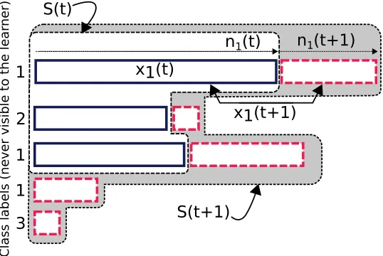
The online problem is formulated as follows. Consider the infinite matrix X given by (7). At every time stept∈N, a part S(t) of X is observed corresponding to the firstN(t) ∈N rows of X, each of lengthni(t), i∈1..N(t), i.e.
S(t) ={xt
1,· · ·xtN(t)} wherexti :=X1i..ni(t).
This setting is depicted in Figure 1. We assume that the number of samples, as well as the individual sample-lengths grow with time. That is, the lengthni(t) of each sequencexi
is nondecreasing and grows to infinity (as a function of time t). The number of sequences N(t) also grows to infinity. Aside from these assumptions, the functionsN(t) andni(t) are
completely arbitrary.
1 1 2 1
3
C
la
ss
labels
(n
ever
vi
si
ble t
o
th
e
lea
rn
er
)
n1(t+1)
n1(t)
x1(t+1) x1(t)
S(t)
S(t+1)
Figure 1: Online Protocol: solid rectangles correspond to sequences available at time t, dashed rectangles correspond to segments arrived at timet+ 1.
An online clustering function is strongly asymptotically consistent if, with probability 1, for each N ∈ N from some time on the first N sequences are clustered correctly (with respect to the ground-truth given by Definition 7).
Definition 9 (Consistency: online setting) A clustering function is strongly (weakly) asymptotically consistent in the online sense, if for everyN ∈N the clusteringf(S(t), κ)|N
is strongly (weakly) asymptotically consistent in the offline sense, where f(S(t), κ)|N is the clustering f(S(t), κ) restricted to the first N sequences:
Remark 10 Note that even if theeventualnumber κ of different time-series distributions producing the sequences (that is, the number of clusters in the ground-truth clustering G) is known, the number of observed distributions at each individual time step is unknown. That is, it is possible that at a given timet we have G|N(t)
< κ.
Known and unknown κ. As mentioned in the introduction, in the general framework de-scribed above, consistent clustering (for both the offline and the online problems) with unknown number of clusters is impossible. This follows from the impossibility result of Ryabko (2010c) that states that when we have only two (binary-valued) samples generated (independently) by two stationary ergodic distributions, it is impossible to decide whether they have been generated by the same or by different distributions, even in the sense of weak asymptotic consistency. (This holds even if the distributions come from a smaller class: the set of all B-processes.) Therefore, if the number of clusters is unknown, we are bound to make stronger assumptions. Since our main interest in this paper is to develop consistent clustering algorithms under the general framework described above, for the most part of this paper we assume that the correct number κ of clusters is known. However, in Section 4.3 we also show that under certain mixing conditions on the process distributions that generate the data, it is possible to have consistent algorithms in the case of unknown κ as well.
4. Clustering Algorithms and their Consistency
In this section we present our clustering methods for both the offline and the online settings. The main results, presented in Sections 4.1 (offline) and 4.2 (online), concern the case where the number of clusters κ is known. In Section 4.3 we show that, given the mixing rates of the process distributions that generate the data, it is possible to find the correct number of clustersκand thus obtain consistent algorithms for the case of unknownκ as well. Finally, Section 4.4 considers some extensions of the proposed settings.
4.1 Offline Setting
Given that we have asymptotically consistent estimates ˆd of the distributional distance d, it is relatively simple to construct asymptotically consistent clustering algorithms for the offline setting. This follows from the fact that, since ˆd(·,·) converges to d(·,·), for large enough sequence lengths n the points x1, . . . ,xN have the so-called strict separation
property: the points within each target cluster are closer to each other than to points in any other cluster (on strict separation in clustering see, for example, Balcan et al., 2008). This makes many simple algorithms, such as single or average linkage, or thek-means algorithm with certain initialisations, provably consistent.
the second cluster centre. For eachk= 2..κthekth cluster centre is sought as the sequence with the largest minimum distance from the already assigned cluster centres for 1..k−1. (This initialisation was proposed for use with k-means clustering by Katsavounidis et al., 1994.) By the last iteration we have κ cluster centres. Next, the remaining samples are each assigned to the closest cluster.
Algorithm 1 Offline clustering
1: INPUT: sequences S:={x1,· · ·,xN}, Number κ of clusters 2: Initialize κ-farthest points as cluster-centres:
3: c1 ←1
4: C1← {c1}
5: for k= 2..κ do
6: ck←argmax i=1..N
min
j=1..k−1 ˆ
d(xi,xcj), where ties are broken arbitrarily
7: Ck← {ck} 8: end for
9: Assign the remaining points to closest centres:
10: for i= 1..N do
11: k←argminj∈Sκ
k=1Ckdˆ(xi,xj)
12: Ck ←Ck∪ {i} 13: end for
14: OUTPUT: clusters C1, C2,· · · , Cκ
Theorem 11 Algorithm 1 is strongly asymptotically consistent (in the offline sense of Def-inition 8), provided that the correct numberκ of clusters is known, and the marginal distri-bution of each sequence xi, i= 1..N is stationary ergodic.
Proof To prove the consistency statement we use Lemma 5 to show that if the samples in S are long enough, the samples that are generated by the same process distribution are closer to each other than to the rest of the samples. Therefore, the samples chosen as cluster centres are each generated by a different process distribution, and since the algorithm assigns the rest of the samples to the closest clusters, the statement follows. More formally, let ndenote the shortest sample length in S:
nmin:= min
i∈1..Nni.
Denote by δ the minimum nonzero distance between the process distributions:
δ := min
k6=k0∈1..κ
ˆ
d(ρk, ρk0).
Fix ε ∈ (0, δ/4). Since there are a finite number N of samples, by Lemma 5 for all large enoughnmin we have
sup
k∈1..κ i∈Gk∩{1..N}
ˆ
where Gk, k = 1..κ denote the ground-truth partitions given by Definition 7. By (8) and applying the triangle inequality we obtain
sup
k∈1..κ i,j∈Gk∩{1..N}
ˆ
d(xi,xj)≤2ε. (9)
Thus, for all large enoughnmin we have inf
i∈Gk∩{1..N}
j∈Gk0∩{1..N}
k6=k0∈1..κ
ˆ
d(xi,xj)≥ inf i∈Gk∩{1..N}
j∈Gk0∩{1..N}
k6=k0∈1..κ
d(ρk, ρk0)−dˆ(xi, ρk)−dˆ(xj, ρk0)
≥δ−2ε (10)
where the first inequality follows from the triangle inequality, and the second inequality follows from (8) and the definition of δ. In words, (9) and (10) mean that the samples in S that are generated by the same process distribution are closer to each other than to the rest of the samples. Finally, for all nmin large enough to have (9) and (10) we obtain
max
i=1..Nk=1min..κ−1 ˆ
d(xi,xck)≥δ−2ε > δ/2
where as specified by Algorithm 1, c1 := 1 and ck := argmax i=1..N
min
j=1..k−1 ˆ
d(xi,xcj), k = 2..κ. Hence, the indices c1, . . . , cκ will be chosen to index sequences generated by different
pro-cess distributions. To derive the consistency statement, it remains to note that, by (9) and (10), each remaining sequence will be assigned to the cluster centre corresponding to the sequence generated by the same distribution.
4.2 Online Setting
The online version of the problem turns out to be more complicated than the offline one. The challenge is that, since new sequences arrive (potentially) at every time step, we can never rely on the distance estimates corresponding to all of the observed samples to be correct. Thus, as mentioned in the introduction, the main challenge can be identified with what we regard as “bad” sequences: recently-observed sequences, for which sufficient information has not yet been collected, and for which the estimates of the distance (with respect to any other sequence) are bound to be misleading. Thus, in particular, farthest-point initialisation would not work in this case. More generally, using any batch algorithm on all available data at every time step results in not only mis-clustering “bad” sequences, but also in clustering incorrectly those for which sufficient data are already available.
Algorithm 2 Online Clustering
1: INPUT: Numberκ of target clusters
2: fort= 1..∞ do
3: Obtain new sequences S(t) ={xt
1,· · ·,xtN(t)}
4: Initialize the normalization factor: η←0
5: Initialize the final clusters: Ck(t)←∅, k = 1..κ
6: Generate N(t)−κ+ 1candidate cluster centres:
7: for j=κ..N(t) do
8: {C1j, . . . , Cκj} ←Alg1({xt1,· · · ,xtj}, κ)
9: µk←min{i∈Ckj}, k= 1..κ . Set the smallest index as cluster centre.
10: (cj1, . . . , cjκ)←sort(µ1, . . . , µκ) . Sort the cluster centres increasingly.
11: γj ←mink6=k0∈1..κdˆ(xt cjk,x
t cj
k0
) .Calculate performance score.
12: wj ←1/j(j+ 1)
13: η←η+wjγj
14: end for
15: Assign points to clusters:
16: for i= 1..N(t)do
17: k←argmink0∈1..κ 1 η
PN(t)
j=1 wjγjdˆ(xti,xtcj k0
)
18: Ck(t)←Ck(t)∪ {i}
19: end for
20: OUTPUT:{C1(t),· · · , Ck(t)}
21: end for
However, the difference here is that the performance of each clustering cannot be measured directly.
More precisely, Algorithm 2 works as follows. Given a set S(t) of N(t) samples, the algorithm iterates over j := κ, . . . , N(t) where at each iteration Algorithm 1 is used to cluster the firstj sequences{xt
1, . . . ,xtj} intoκ clusters. In each cluster the sequence with
the smallest index is assigned as the candidate cluster centre. A performance score γj is
calculated as the minimum distance ˆdbetween theκ candidate cluster centres obtained at iteration j. Thus, γj is an estimate of the minimum inter-cluster distance. At this point
we haveN(t)−κ+ 1 sets of κ cluster centres c1j, . . . , cjκ, j = 1..N(t)−κ+ 1. Next, every
sample xti, i = 1..N(t) is assigned to a cluster, according to the weighted combination of the distances betweenxti and the candidate cluster centres obtained at each iteration onj. More precisely, for eachi= 1..N(t) the sequencexti is assigned to the cluster κ, whereκ is defined as
k:= argmink=1..κ
N(t) X
j=κ
wjγjdˆ(xti,xtcj k
).
Before giving the proof of Theorem 12, we provide an intuitive explanation as to how Algorithm 2 works. First, consider the following simple candidate solution. Take some fixed (reference) portion of the samples, run the batch algorithm on it, and then simply assign every remaining sequence to the nearest cluster. Since the offline algorithm is asymptotically consistent, this procedure would be asymptotically consistent as well, but only if we knew that the selected reference of the sequences contains at least one sequence sampled from each and every one of the κ distributions. However, there is no way to find a fixed (not growing with time) portion of data that would be guaranteed to contain a representative of each cluster (that is, of each time-series distribution). Allowing such a reference set of sequences to grow with time would guarantee that eventually it contains representatives of all clusters, but it would break the consistency guarantee for the reference set; since the set grows, this formulation effectively returns us back to the original online clustering problem. A key observation we make to circumvent this problem is the following. If, for some j ∈ {κ, . . . , N(t)}, each sample in the batch {xt
1, . . . ,xtj} is generated by at most κ−1
process distributions, any partitioning of this batch into κsets results in a minimum inter-cluster distance γj that, as follows from the asymptotic consistency of ˆd, converges to 0.
On the other hand, if the set of samples {xt
1, . . . ,xtj} contains sequences generated by all
κ process distributions,γj converges to a nonzero constant, namely, the minimum distance
between the distinct process distributions ρ1, . . . , ρκ. In the latter case from some time on
the batch {xt
1, . . . ,xtj} will be clustered correctly. Thus, instead of selecting one reference
batch of sequences and constructing a set of clusters based on those, we consider all batches of sequences for j = κ..N(t), and combine them with weights. Two sets of weights are involved in this step: γj andwj, where
1. γj is used to penalise for small inter-cluster distance, cancelling the clustering results
produced based on sets of sequences generated by less thanκ distributions;
2. wjis used to give precedence to chronologically earlier clusterings, protecting the
clus-tering decisions from the presence of the (potentially “bad”) newly formed sequences, whose corresponding distance estimates may still be far from accurate.
As time goes on, the batches in which not all clusters are represented will have their weight γj converge to 0, while the number of batches that have all clusters represented and are
clustered correctly by the offline algorithm will go to infinity, and their total weight will approach 1. Note that, since we are combining different clusterings, it is important to use a consistent ordering of clusters, for otherwise we might sum up clusters generated by different distributions. Therefore, we always order the clusters with respect to the index of the first sequence in each cluster.
Proof [of Theorem 12] First, we show that for everyk∈1..κwe have
1 η
N(t) X
j=1
wjγjtdˆ(xtcj k
, ρk)→0 a.s. (11)
Denote by δ the minimum nonzero distance between the process distributions:
δ := min
k6=k0∈1..κ
ˆ
Fixε∈(0, δ/4). We can find an indexJ such thatP∞
j=Jwj ≤ε. LetS(t)|j ={xt1,· · · ,xtj}
denote the subset ofS(t) consisting of the firstj sequences forj∈1..N(t). Fork= 1..κlet
sk:= min{i∈ Gk∩1..N(t)} (13)
index the first sequence inS(t) that is generated by ρk whereGk, k= 1..κare the
ground-truth partitions given by Definition 7. Define
m:= max
k∈1..κsk. (14)
Recall that the sequence lengthsni(t) grow with time. Therefore, by Lemma 5 (consistency
of ˆd) for everyj∈1..J there exists someT1(j) such that for all t≥T1(j) we have sup
k∈1..κ i∈Gk∩{1..j}
ˆ
d(xti, ρk)≤ε. (15)
Moreover, by Theorem 11 for everyj∈m..Jthere exists someT2(j) such that Alg1(S(t)|j, κ)
is consistent for allt≥T2(j). Let
T := max
i=1,2
j∈1..J
Ti(j).
Recall that, by definition (14) ofm,S(t)|mcontains samples from allκdistributions. There-fore, for all t≥T we have
inf
k6=k0∈1..κ
ˆ d(xtcm
k ,x
t cm
k0)
≥ inf
k6=k0∈1..κd(ρk, ρk0)− sup k6=k0∈1..κ( ˆd(x
t cm
k , ρk) + ˆd(x
t cm
k0, ρk
0))
≥δ−2ε≥δ/2, (16)
where the first inequality follows from the triangle inequality and the second inequality follows from the consistency of Alg1(S(t)|m, κ) for t≥T, the definition of δ given by (12)
and the assumption that ε ∈ (0, δ/4). Recall that (as specified in Algorithm 2) we have η:=PN(t)
j=1 wjγjt. Hence, by (16) for allt≥T we have
η ≥wmδ/2. (17)
By (17) and noting that by definition, ˆd(·,·)≤1 for allt≥T, for everyk∈1..κwe obtain
1 η
N(t) X
j=1
wjγjtdˆ(xtcj k
, ρk)≤
1 η
J
X
j=1
wjγjtdˆ(xtcj k
, ρk) +
2ε wmδ
. (18)
On the other hand, by the definition (14) ofm, the sequences inS(t)|j forj= 1..m−1 are
generated byat most κ−1 out of theκprocess distributions. Therefore, at every iteration onj∈1..m−1 there exists at least one pair of distinct cluster centres that are generated by
the same process distribution. Therefore, by (15) and (17), for allt≥T and everyk∈1..κ we have,
1 η
m−1 X
j=1
wjγjtdˆ(xtcj k
, ρi)≤
1 η
m−1 X
j=1
wjγjt≤
2ε wmδ
Noting that the clusters are ordered in the order of appearance of the distributions, we have xt
cjk =x t
sk for allj =m..J and k= 1..κ, where the index sk is defined by (13). Therefore, by (15) for allt≥T and everyk= 1..κwe have
1 η
J
X
j=m
wjγjtdˆ(xtcj k
, ρk) =
1 ηdˆ(x
t sk, ρk)
J
X
j=m
wjγjt≤ε. (20)
Combining (18), (19), and (20) we obtain
1 η
N(t) X
j=1
wjγjtdˆ(xtcj k
, ρk)≤ε(1 +
4 wmδ
). (21)
for all k= 1..κand allt≥T, establishing (11).
To finish the proof of the consistency, consider an index i ∈ Gr for some r ∈ 1..κ. By Lemma 5, increasingT if necessary, for all t≥T we have
sup
k∈1..κ j∈Gk∩1..N
ˆ
d(xtj, ρk)≤ε. (22)
For allt≥T and all k6=r∈1..κwe have,
1 η
N(t) X
j=1
wjγjtdˆ(xti,xtcj k
)≥ 1 η
N(t) X
j=1
wjγjtdˆ(xti, ρk)−
1 η
N(t) X
j=1
wjγjtdˆ(xtcj k
, ρk)
≥ 1 η
N(t) X
j=1
wjγjt( ˆd(ρk, ρr)−dˆ(xti, ρr))−
1 η
N(t) X
j=1
wjγjtdˆ(xtcj k
, ρk)
≥δ−2ε(1 + 2 wmδ
), (23)
where the first and second inequalities follow from the triangle inequality, and the last inequality follows from (22), (21) and the definition ofδ. Since the choice ofεis arbitrary, from (22) and (23) we obtain
argmin
k∈1..κ
1 η
N(t) X
j=1
wjγjtdˆ(xti,xtcj k
) =r. (24)
It remains to note that for any fixedN ∈Nfrom someton (24) holds for alli= 1..N, and the consistency statement follows.
4.3 Unknown Number κ of Clusters
of Ryabko (2010c) discussed in Section 3, the correct numberκof clusters is not possible to be estimated with no further assumptions or additional constraints. One way to overcome this obstacle is to assume known rates of convergence of frequencies to the corresponding probabilities. Such rates are provided by assumptions on the mixing rates of the process distributions that generate the data.
Here we will show that under some assumptions on the mixing rates (and still without making any modelling or independence assumptions), consistent clustering is possible when the number of clusters is unknown.
The purpose of this section, however, is not to find the weakest assumptions under which consistent clustering (withκ unknown) is possible, nor is it to provide sharp bounds under the assumptions considered; our only purpose here is to demonstrate that asymptotic consistency is achievable in principle when the number of clusters is unknown, under some mild nonparametric assumptions on the time-series distributions. More refined analysis could yield sharper bounds under weaker assumptions, such as those in, for example, (Bosq, 1996; Rio, 1999; Doukhan, 1994; Doukhan et al., 2010).
We introduce mixing coefficients, mainly following Rio (1999) in formulations. Infor-mally, mixing coefficients of a stochastic process measure how fast the process forgets about its past. Any one-way infinite stationary process X1, X2, . . . can be extended backwards to make a two-way infinite process . . . , X−1, X0, X1, . . . with the same distribution. In the definition below we assume such an extension. Define theϕ-mixing coefficients of a process µas
ϕn(µ) = sup
A∈σ(X−∞..k),B∈σ(Xk+n..∞),µ(A)6=0
|µ(B|A)−µ(B)|, (25)
where σ(..) stands for the σ-algebra generated by random variables in brackets. These coefficients are nonincreasing. Define also
θn(µ) := 2 + 8(ϕ1(µ) +· · ·+ϕn(µ)).
A processµis called uniformlyϕ-mixingifϕn(µ)→0. Many important classes of processes
satisfy mixing conditions. For example, a stationary irreducible aperiodic Hidden Markov process with finitely many states is uniformly ϕ-mixing with coefficients decreasing expo-nentially fast. Other probabilistic assumptions can be used to obtain bounds on the mixing coefficients, see, e.g., (Bradley, 2005) and references therein.
The method that we propose for clustering mixing time series in the offline setting, namelyAlgorithm 3, is very simple. Its inputs are: a setS:={x1, . . . ,xN}of samples each
of length ni, i= 1..N, the threshold levelδ ∈(0,1) and the parameters m, l ∈N, Bm,l,n.
The algorithm assigns to the same cluster all samples which are at most δ-far from each other, as measured by ˆd with mn = m, ln =l and the summation over Bm,l restricted to
Bm,l,n. The setsBm,l,nhave to be chosen so that in asymptotic they cover the whole space, ∪n∈NBm,l,n=Bm,l. For example,Bm,l,nmay consist of the firstbncubes around the origin,
where bn → ∞ is a parameter sequence. We do not give a pseudocode implementation of
this algorithm, since it is rather clear.
The idea is that the threshold level δ=δnis selected according to the smallest
sample-lengthn:= mini=1..Nniand the (known bounds on) mixing rates of the processρgenerating
the parameters of Algorithm 3 in such a way that it is weakly asymptotically consistent. Moreover, a bound on the probability of error before asymptotic is provided.
Theorem 13 (Algorithm 3 is consistent for unknown κ) Fix sequences mn, ln, bn ∈
N, and let, for each m, l∈ N, Bm,l,n ⊂Bm,l be an increasing sequence of finite sets such
that ∪n∈NBm,l,n = Bm,l. Set bn := maxl≤ln,m≤mn|B
m,l,n| and n:= min
i=1..Nni. Let also
δn ∈ (0,1). Let N ∈ N, and suppose that the samples x1, . . . ,xN are generated in such a way that the (unknown marginal) distributions ρk, k = 1..κ are stationary ergodic and satisfy ϕn(ρk)≤ϕn, for all k= 1..κ, n∈N. Then there exist constants ερ, δρ andnρ that depend only on ρk, k= 1..κ, such that for all δn< δρ and n > nρ, Algorithm 3 satisfies
P(T 6=G|N)≤2N(N + 1)(mnlnbnγn/2(δn) +γn/2(ερ)) (26) where
γn(ε) :=
√
eexp(−nε2/θn),
T is the partition output by the algorithm andG|N is the ground-truth clustering. In partic-ular, ifϕn=o(1), then, selecting the parameters in such a way that δn=o(1), mn, ln, bn=
o(n), mn, ln→ ∞, ∪k∈NBm,l,k =Bm,l, b m,l
n → ∞, for all m, l∈N, γn(const) =o(1), and, finally, mnlnbnγn(δn) = o(1), as is always possible, Algorithm 3 is weakly asymptotically
consistent(with the number of clusters κ unknown).
Proof We use the following bound from (Rio, 1999, Corollary 2.1): for any zero-mean [−1,1]-valued random processY1, Y2, . . . with distribution P and everyn∈Nwe have
P |
n
X
i=1
Yi|> nε
!
≤γn(ε). (27)
For every j = 1..N, every m < n, l∈N, andB ∈Bm,l, define the [−1,1]-valued processes Yj :=Y1j, Y2j, . . . as
Ytj :=I{(Xtj, . . . , X j
t+m−1)∈B} −ρk(X1j..m ∈B),
where ρk is the marginal distribution of Xj (that is, k is such that j ∈ Gk). It is easy to
see thatϕ-mixing coefficients for this process satisfyϕn(Yj)≤ϕn−2m. Thus, from (27) we
have
P(|ν(X1j..nj, B)−ρk(X1j..m∈B)|> ε/2)≤γn−2mn(ε/2). (28) Then for every i, j ∈ Gk∩1..N for some k ∈ 1..κ (that is, xi and xj are in the same
ground-truth cluster) we have
P(|ν(X1i..ni, B)−ν(X1j..nj, B)|> ε)≤2γn−2mn(ε/2). Using the union bound, summing over m, l, andB, we obtain
Next, let i∈ Gk∩1..N and j ∈ Gk0 ∩1..N for k6=k0 ∈1..κ(i.e., xi,xj are in two different
target clusters). Then, for some mi,j, li,j ∈ N there is Bi,j ∈ Bmi,j,li,j such that for some
τi,j >0 we have
|ρk(X1i..|Bi,j|∈Bi,j)−ρk0(X
j
1..|Bi,j|∈Bi,j)|>2τi,j. Then for everyε < τi,j/2 we have
P(|ν(X1i..ni, Bi,j)−ν(X1j..nj, Bi,j)|< ε)≤2γn−2mi,j(τi,j). (30) Moreover, for ε < wmi,jwli,jτi,j/2 we have
P( ˆd(xi,xj)< ε)≤2γn−2mi,j(τi,j). (31) Define
δρ:= min k6=k0∈1..κ i∈Gk∩1..N
j∈Gk0∩1..N
wmi,jwli,jτi,j/2, ερ:= min
k6=k0∈1..κ i∈Gk∩1..N
j∈Gk0∩1..N
τi,j/2
nρ:= 2 max k6=k0∈1..κ i∈Gk∩1..N
j∈Gk0∩1..N
mi,j.
Clearly, from this and (30), for every δ <2δρ and n > nρ we obtain
P( ˆd(xi,xj)< δ)≤2γn/2(ερ). (32)
Algorithm 3 produces correct results if for every pairi, j we have ˆd(xi,xj)< δnif and only
if i, j∈ Gk∩1..N for some k ∈1..κ. Therefore, taking the bounds (29) and (32) together for each of the N(N + 1)/2 pairs of samples, we obtain (26).
For the online setting, consider the following simple extension of Algorithm 3, that we call Algorithm 3’. It applies Algorithm 3 to the first Nt sequences, where the parameters
of Algorithm 3 and Nt are chosen in such a way that the bound (26) with N =Nt is o(1)
and Nt → ∞ as time t goes to infinity. It then assigns each of the remaining sequences
(xi, i > Nt) to the nearest cluster. Note that in this case the bound (26) with N = Nt
bounds the error of Algorithm 3’ on the firstNt sequences, as long as all of theκ clusters
are already represented among the firstNtsequences. SinceNt→ ∞, we can formulate the
following result.
Theorem 14 Algorithm 3’ is weakly asymptotically consistent in the online setting when the numberκ of clusters is unknown, provided that the assumptions of Theorem 13 apply to the first N sequences x1, . . . ,xN for everyN ∈N.
4.4 Extensions
4.4.1 AMS Processes and Gradual Changes
Here we argue that our results can be strengthened to a more general case where the process distributions that generate the data are Asymptotically Mean Stationary (AMS) ergodic. Throughout the paper we have been concerned with stationary ergodic process distributions. Recall from Section 2 that a process ρ is stationary if for any i, j ∈ 1..n and B ∈ Bm, m ∈ N, we have ρ(X1..j ∈ B) = ρ(Xi..i+j−1 ∈ B). A stationary process is called ergodic if the limiting frequencies converge to their corresponding probabilities, so that for all B ∈ B with probability 1 we have limn→∞ν(X1..n, B) = ρ(B). This latter
convergence of all frequencies is the only property of the process distributions that is used in the proofs (via Lemma 5) which give rise to our consistency results. We observe that this property also holds for a more general class of processes, namely those that are AMS ergodic. Specifically, a process ρ is called AMS if for every j∈1..n and B ∈Bm, m Nthe series limn→∞Pni=1−j+1 1nρ(Xi..i+j−1∈B) converges to a limit ¯ρ(B), which forms a measure, i.e. ¯ρ(X1..j ∈B) := ¯ρ(B),B ∈Bm, m∈N, called asymptotic mean of ρ. Moreover, if ρ is an AMS process, then for everyB ∈Bm, m∈N, the frequencyν(X1..n, B) convergesρ-a.s.
to a random variable with mean ¯ρ(B). Similarly to stationary processes, if the random variable to whichν(X1..n, B) converges is a.s. constant, thenρ is called AMS ergodic. More
information on AMS processes can be found in the work (Gray, 1988). However, the main characteristic pertaining to our work is that the class of all processes with AMS properties is composed precisely of those processes for which the almost sure convergence of frequencies to the corresponding probabilities holds. It is thus easy to check that all of the asymptotic results of Sections 4.1, 4.2 carry over to the more general setting where the unknown process distributions that generate the data are AMS ergodic.
4.4.2 Strictly Separated Clusters of Distributions
So far we have defined a cluster as a set of sequences generated by the same distribution. This seems to capture rather well the notion that in the same cluster the objects can be very different (as is the case for stochastically generated sequences), yet are intrinsically of the same nature (they have the same law).
However, one may wish to generalise this further, and allow each sequence to be gener-ated by a different distribution, yet requiring that in the same clusters distributions must be close. Unlike the original formulation, such an extension would require fixing some sim-ilarity measure between distributions. The results of the preceding sections suggest using the distributional distance for this purpose.
Specifically, as discussed in Section 4.1, in our formulation, from some time on, the sequences possess the so-called strict separation property in the ˆd distance: sequences in the same target cluster are closer to each other than to those in other clusters. One possible way to relax the considered setting is to impose the strict separation property on the distributions that generate the data. Here the separation would be with respect to the distributional distanced. That is, each sequencexi, i= 1..N, may be generated by its own
distributionρi, but the distributions{ρi:i= 1..N}can be clustered in such a way that the
to the online setting remains open. For the offline case, we can formulate the following result, whose proof is analogous to that of Theorem 11.
Theorem 15 Assume that each sequencexi, i= 1..N is generated by a stationary ergodic distribution ρi. Assume further that the set of distributions {1, . . . , N} admits a parti-tioning G = {G1, . . . ,Gk} that has the strict separation property with respect to d: for all
i, j = 1..k, i 6= j, for all ρ1, ρ2 ∈ Gi and all ρ3 ∈ Gj we have d(ρ1, ρ2) < d(ρ1, ρ3). Then
Algorithm 1 is strongly asymptotically consistent, in the sense that almost surely from some
n= min{n1, . . . , nN} on it outputs the set G. 5. Computational Considerations
In this section we show that all of the proposed methods are efficiently computable. This claim is further illustrated by the experimental results in the next section. Note, however, that since the results presented are asymptotic, the question of what is the best achievable computational complexity of an algorithm that still has the same asymptotic performance guarantees is meaningless: for example, an algorithm could throw away most of the data and still be asymptotically consistent. This is why we do not attempt to find a resource-optimal way of computing the methods presented.
First, we show that calculating ˆd is at most quadratic (up to log terms), and quasilinear if we use mn = logn. Let us begin by showing that calculating ˆd is fully tractable with
mn, ln≡ ∞. First, observe that for fixedm and l, the sum
Tm,l:= X
B∈Bm,l
|ν(X11..n1, B)−ν(X12..n2, B)| (33)
has not more thann1+n2−2m+ 2 nonzero terms (assumingm≤n1, n2; the other case is obvious). Indeed, there areni−m+ 1 tuples of sizemin each sequencexi, i= 1,2 namely,
X1i..m, X2i..m+1, . . . , Xni1−m+1..n1. Therefore, Tm,l can be obtained by a finite number of calculations.
Furthermore, let
s= min
X1
i6=Xj2
i=1..n1,j=1..n2
|Xi1−Xj2|, (34)
and observe that Tm,l= 0 for all m > n and for each m, for all l >logs−1 the term Tm,l is constant. That is, for each fixedm we have
∞ X
l=1
wmwlTm,l=wmwlogs−1Tm,logs
−1
+ logs−1
X
l=1
wmwlTm,l
so that we simply double the weight of the last nonzero term. (Note also thatsis bounded above by the length of the binary precision in representing the random variablesXji.) Thus, even withmn, ln≡ ∞one can calculate ˆdprecisely. Moreover, for a fixedm∈1..lognand
l ∈ 1..logs−1 for every sequence xi, i = 1,2 the frequencies ν(xi, B), B ∈ Bm,l may
subsequences of length m results in O(m+z) = O(n) complexity. This brings the overall computational complexity of (3) toO(nmnlogs−1); this can potentially be improved using
specialized structures, e.g., (Grossi and Vitter, 2005).
The following consideration can be used to set mn. For a fixed l the frequencies
ν(xi, B), i= 1,2 of cells in B ∈Bm,l corresponding to values of m much larger than logn
(in the asymptotic sense, that is, if logn = o(m)) are not, in general, consistent estimates of their probabilities, and thus only add to the estimation error. More specifically, for a subsequenceXj..j+mwithj= 1..n−mof lengthmthe probabilityρi(Xj..j+m∈B), i= 1,2
is of order 2−mhi, i= 1,2 whereh
idenotes the entropy rate ofρi, i= 1,2. Moreover, under
some (general) conditions (includinghi>0) one can show that, asymptotically, a string of
length of order logn/hi on average occurs at most once in a string of lengthn(Kontoyiannis
and Suhov, 1994). Therefore, subsequences of length m larger than logn are typically met 0 or 1 times, and thus are not consistent estimates of probabilities. By the above argument, one can usemn of order logn. To chooseln<∞one can either fix some constant based on
the bound on the precision in real computations, or choose it in such a way that each cell Bm,ln contains no more than lognpoints for allm= 1..lognlargest values ofl
n.
5.1 Complexity of the Algorithms.
The computational complexity of the presented algorithms is dominated by the complexity of calculations of ˆdbetween different pairs of sequences. Thus, it is sufficient to bound the number of pairwise ˆdcomputations.
It is easy to see that the offline algorithm for the case of known κ (Algorithm 1) re-quires at most κN distance calculations, while for the case of unknown κ all N2 distance calculations are necessary.
The computational complexity of the updates in the online algorithm can be computed as follows. Assume that the pairwise distance values are stored in a database D, and that for every sequencexti−1, i∈Nwe have already constructed a suffix tree, using for example, the online algorithm of Ukkonen (1995). At time step t, a new symbol X is received. Let us first calculate the required computations to update D. We have two cases, either X forms a new sequence, so that N(t) = N(t−1) + 1, or it is the subsequent element of a previously received segment, say, xtj for some j ∈ 1..N(t), so that nj(t) = nj(t−1) + 1.
In either case, let xtj denote the updated sequence. Note that for all i 6= j ∈ 1..N(t) we have ni(t) =ni(t−1). Recall the notation xti:=X
(i) 1 , . . . X
(i)
ni(t) fori∈1..N(t). In order to update D we need to update the distance between xt
j and xti for all i6= j ∈ N(t). Thus,
we need to search for all mn new patterns induced by the received symbol X, resulting in
complexity at mostO(N(t)m2nln). Letn(t) := max{n1(t), . . . nN(t)(t)}, t∈N. As discussed previously, we letmn:= logn(t); we also define ln:= logs(t)−1 where
s(t) := min
i,j∈1..N(t)
u=1..ni(t),v=1..nj(t),Xu(i)6=Xv(j)
|Xu(i)−Xv(j)|, t∈N.
of order equivalent to its complete construction, resulting in a computational complexity of order O(N(t)n(t) log2n(t)). Therefore, we avoid calculating s(t) at every time step; instead, we update s(t) at prespecified time steps so that for every n(t) symbols received, Dis reconstructed at most logn(t) times. (This can be done, for example, by recalculating s(t) at time steps wheren(t) is a power of 2.) It is easy to see that with the database Dof distance values at hand, the rest of the computations are of order at mostO(N(t)2). Thus, the computational complexity of updates in Algorithm 2 is at mostO(N(t)2+N(t) log3n(t)).
6. Experimental Results
In this section we present empirical evaluations of Algorithms 1 and 2 on both synthetically generated and real data.
6.1 Synthetic Data
We start with synthetic experiments. In order for the experiments to reflect the generality of our approach we have selected time-series distributions that, while being stationary ergodic, cannot be considered as part of any of the usual smaller classes of processes, and are difficult to approximate by finite-state models. Namely, we consider rotation processes used, for example, by Shields (1996) as an example of stationary ergodic processes that are not B -processes. Such time series cannot be modelled by a hidden Markov model with a finite or countably infinite set of states. Moreover, while k-order Markov (or hidden Markov) approximations of this process converge to it in the distributional distance d, they do not converge to it in the ¯ddistance, a stronger distance thandwhose empirical approximations are often used to study general (non-Markovian) processes (e.g., Ornstein and Weiss, 1990).
6.1.1 Time Series Generation
To generate a sequence x = X1..n we proceed as follows: Fix some parameter α ∈ (0,1).
Select r0 ∈ [0,1]; then, for each i = 1..n obtain ri by shifting ri−1 by α to the right, and removing the integer part, i.e. ri:=ri−1+α− bri−1+αc. The sequencex= (X1, X2,· · ·) is then obtained from ri by thresholding at 0.5, that isXi :=I{ri>0.5}. Ifα is irrational
thenxforms a stationary ergodic time series. (We simulateα by alongdoublewith a long mantissa.)
For the purpose of our experiments, first we fix κ:= 5 difference process distributions specified by α1 = 0.31..., α2 = 0.33..., α3 = 0.35..., α4 = 0.37..., α5= 0.39.... The param-eters αi are intentionally selected to be close, in order to make the process distributions
harder to distinguish. Next we generate an N ×M data matrix X, each row of which is a sequence generated by one of the process distributions. Our task in both the online and the batch setting is to cluster the rows of X intoκ= 5 clusters.
6.1.2 Batch Setting
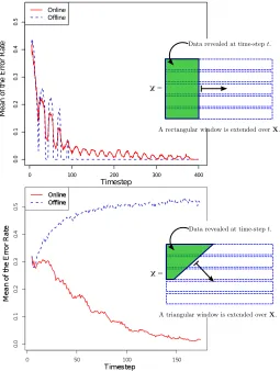
each of the algorithms, (online and offline) cluster the rows ofX|n(t) into five clusters, and calculate the clustering error rate of each algorithm. As shown in Figure 2 (top) the error rate of each algorithm decreases with sequence length.
0 100 200 300 400
0.
0
0.
1
0.
2
0.
3
0.
4
0.
5
Timestep
M
ea
n
of
th
e
E
rr
or
R
at
e
Online Offline
Figure 2: Top: error rate vs. sequence length in batch setting. Bottom: error rate vs. Number of observed samples in online setting. (error rates averaged over 100 runs.)
6.1.3 Online Setting
In this experiment we demonstrate that, unlike the online algorithm, the offline algorithm is consistently confused by the new sequences arriving at each time step in an online setting. To simulate an online setting, we proceed as follows: At every time step t, a triangular window is used to reveal the first 1..ni(t), i= 1..t elements of the firstt rows of the data
matrix X, with ni(t) := 5(t−i) + 1, i = 1..t. This gives a total of t sequences, each of
lengthni(t), fori= 1..t, where the ith sequence fori= 1..tcorresponds to theith row ofX
terminated at lengthni(t). At every time step t the online and offline algorithms are each
of both algorithms is measured on all sequences available at a given time, not on a fixed batch of sequences. As shown in Figure 2 (bottom), in this setting the clustering error rate of the offline algorithm remains consistently high, whereas that of the online algorithm converges to zero.
6.2 Real Data
As an application we consider the problem of clustering motion capture sequences, where groups of sequences with similar dynamics are to be identified. Data is taken from the Motion Capture database (MOCAP) which consists of time-series data representing human locomotion. The sequences are composed of marker positions on human body which are tracked spatially through time for various activities.
We compare our results to those obtained with two other methods, namely those of Li and Prakash (2011) and Jebara et al. (2007). Note that we have not implemented these reference methods, rather we have taken the numerical results directly from the correspond-ing articles. In order to have common grounds for each comparison we use the same sets of sequences2 and the same means of evaluation as those used by Li and Prakash (2011); Jebara et al. (2007).
In the paper by Li and Prakash (2011) two MOCAP data sets3 are used, where the sequences in each data set are labelled with either running or walking as annotated in the database. Performance is evaluated via the conditional entropy S of the true labelling with respect to the prediction, i.e., S := −P
i,j
Mij
P
i0,j0Mi0j0 log Mij
P
j0Mij0 where M denotes the clustering confusion matrix. The motion sequences used by Li and Prakash (2011) are reportedly trimmed to equal duration. However, we use the original sequences as our method is not limited by variation in sequence lengths. Table 1 lists performance of Algorithm 1 as well as that reported for the method of Li and Prakash (2011); Algorithm 1 performs consistently better.
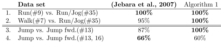
In the paper (Jebara et al., 2007) four MOCAP data sets4 are used, corresponding to four motions: run, walk, jump and forward jump. Table 2 lists performance in terms of accuracy. The data sets in Table 2 constitute two types of motions:
1. motions that can be considered ergodic: walk, run, run/jog (displayed above the double line), and
2. non-ergodic motions: single jumps (displayed below the double line).
As shown in Table 2, Algorithm 1 achieves consistently better performance on the first group of data sets, while being competitive (better on one and worse on the other) on the non-ergodic motions. The time taken to complete each task is in the order of few minutes on a standard laptop computer.
2. The subject’s right foot was used as marker position. 3. The corresponding subject references are #16 and #35.