Analysis of Classification-based Policy Iteration Algorithms
Alessandro Lazaric1 [email protected]
Mohammad Ghavamzadeh2,1 [email protected]
R´emi Munos3,1 [email protected]
1 INRIA Lille - Team SequeL, France
2 Adobe Research, USA
3 Google DeepMind, UK
Editor:Shie Mannor
Abstract
We introduce a variant of the classification-based approach to policy iteration which uses a cost-sensitive loss function weighting each classification mistake by its actualregret, that is, the difference between the action-value of the greedy action and of the action chosen by the classifier. For this algorithm, we provide a full finite-sample analysis. Our results state a performance bound in terms of the number of policy improvement steps, the number of rollouts used in each iteration, the capacity of the considered policy space (classifier), and a capacity measure which indicates how well the policy space can approximate policies that are greedy with respect to any of its members. The analysis reveals a tradeoff between the estimation and approximation errors in this classification-based policy iteration setting. Furthermore it confirms the intuition that classification-based policy iteration algorithms could be favorably compared to value-based approaches when the policies can be approxi-mated more easily than their corresponding value functions. We also study the consistency of the algorithm when there exists a sequence of policy spaces with increasing capacity.
Keywords: reinforcement learning, policy iteration, classification-based approach to policy iteration, finite-sample analysis.
1. Introduction
Policy iteration(Howard, 1960) is a method of computing an optimal policy for any given Markov decision process (MDP). It is an iterative procedure that discovers a determin-istic optimal policy by generating a sequence of monotonically improving policies. Each iteration k of this algorithm consists of two phases: policy evaluation in which the action-value function Qπk of the current policy π
k is computed (i.e., the expected sum of
dis-counted rewards collected by acting according to policy πk), and policy improvement in
which the new (improved) policy πk+1 is generated as the greedy policy w.r.t. Qπk, that
si, πk+1(x) = arg maxa∈AQπk(x, a). Unfortunately, in MDPs with large (or continuous)
state and action spaces, the policy evaluation problem cannot be solved exactly and ap-proximation techniques are required. In approximate policy iteration (API), a function
approximation scheme is usually employed in the policy evaluation phase. The most com-mon approach is to find a good approximation of the value function of πk in a real-valued
and its high-quality samples are often very expensive to obtain, if this option is possible at all,2)it is often difficult to find a function space rich enough to represent the action-value function accurately, and thus, careful hand-tuning is needed to achieve satisfactory results,
3)for the success of policy iteration, it is not necessary to estimateQπk accurately at every
state-action pair, what is important is to have an approximation of the action-value func-tion whose greedy policy improves over the previous policy, and 4) this method may not be the right choice in domains where good policies are easier to represent and learn than the corresponding value functions.
To address the above issues, mainly 3 and4,1 variants of
API have been proposed that
replace the usual value function learning step (approximating the action-value function over the entire state-action space) with a learning step in a policy space (Lagoudakis and Parr, 2003b; Fern et al., 2004). The main idea is to cast the policy improvement step as a
classification problem. The training set is generated using rollout estimates of Qπ over a
finite number of states D={xi}N
i=1, called therollout set, and for any action a∈ A.2 For
each x ∈ D, if the estimated value Qbπ(x, a+) for action a+ is greater than the estimated value of all other actions with high confidence, the state-action pair (x, a+) is added to the
training set with a positive label. In this case, (x, a) for the rest of the actions are labeled negative and added to the training set. The policy improvement step thus reduces to solving a classification problem to find a policy in a given hypothesis space that best predicts the greedy action at every state. Although whether selecting a suitable policy space is any easier than a value function space is highly debatable, we can argue that the classification-based
API methods can be advantageous in problems where good policies are easier to represent
and learn than their value functions.
The classification-based API algorithms can be viewed as a type of reduction from
reinforcement learning (RL) to classification, that is, solving a MDP by generating and solving a series of classification problems. There have been other proposals for reducing RL to classification. Langford and Zadrozny (2005) provided a formal reduction from RL to classification, showing that-accurate classification implies near optimal RL. This approach uses an optimistic variant of sparse sampling to generate h classification problems, one for each horizon time step. The main limitation of this work is that it does not provide a practical method for generating training examples for these classification problems. Bagnell et al. (2003) introduced an algorithm, called policy search by dynamic programming (PSDP)
for learning non-stationary policies in RL. For a specified horizonh, their approach learns a sequence of h policies. At each iteration, all policies are fixed except for one, which is optimized by forming a classification problem via policy rollout. Perhaps the closest approach to the classification-based API methods proposed and analyzed in this paper
is the group of algorithms that are introduced and analyzed in (Kakade and Langford, 2002) and (Kakade, 2003) under the name conservative policy iteration(CPI).3 The main
algorithmic difference between CPI and the classification-based API methods studied in
1. The first drawback is shared by all reinforcement learning algorithms and the second one is common to all practical applications of machine learning methods.
this paper is that while the output of the classifier is directly assigned to the next policy in our algorithms,CPI algorithms perform a more conservative policy update in which the
new policy πk+1 is a mixture distribution of the current policy πk and the output of the
classifier (policies might be stochastic). This conservative update gives CPI two desirable
properties: 1) it guarantees to improve the policy at each iteration, that is, the value function of πk+1 is larger than the value function ofπk, and 2)it has a stopping condition
based on the quality of the generated policy (it stops whenever it cannot guarantee that the new policy has a better performance than the previous one). These properties can potentially make CPIa very appealingAPI algorithm, mainly because otherAPImethods
have no guarantee to generate monotonically improving policies and they only converge to a region (i.e., they may repeatedly oscillate among different policies). This includes both value function based API algorithms such as LSPI (Lagoudakis and Parr, 2003a)
and classification-basedAPI methods. However, Ghavamzadeh and Lazaric (2012) showed
that CPI’s desirable properties do not come for free. The analysis of Ghavamzadeh and
Lazaric (2012) reveals that in order to achieve the same level of accuracy,CPIrequires more
iterations, and thus, more samples than the classification-based API algorithms proposed
in this paper. This indicates that although CPI’s conservative update allows it to have a
monotonically improving behavior, it slows down the algorithm and increases its sample complexity. On the other hand, CPI retains the advantage of a concentrability coefficient
(or density ratios), which can be much smaller for CPI whenever prior knowledge about
the stationary distribution of the optimal policy is used to properly tune the sampling distribution.4 Nonetheless, Ghavamzadeh and Lazaric (2012) further show that
CPI may
converge to suboptimal policies whose performance is not better than those returned by the algorithms studied in this paper. Given the advantages and disadvantages, the classification-based API algorithm proposed in this paper and CPI remain two valid alternatives to
implement the general approximate policy iteration scheme.
Although the classification-based API algorithms have been successfully applied to
benchmark problems (Lagoudakis and Parr, 2003b; Fern et al., 2004) and have been modi-fied to become more computationally efficient (Dimitrakakis and Lagoudakis, 2008b), a full theoretical understanding of them is still lacking. Fern et al. (2006) and Dimitrakakis and Lagoudakis (2008a) provide a preliminary theoretical analysis of their algorithm. In partic-ular, they both bound the difference in performance at each iteration between the learned policy and the true greedy policy. Their analysis is limited to one step policy update (they do not show how the error in the policy update is propagated through the iterations of the
API algorithm) and either to finite class of policies (in Fern et al., 2006) or to a specific
architecture (a uniform grid in Dimitrakakis and Lagoudakis, 2008a). Moreover, the bound reported in (Fern et al., 2006) depends inversely on the minimum Q-value gap between a greedy and a sub-greedy action over the state space. In some classes of MDPs this gap can be arbitrarily small so that the learned policy can be arbitrarily worse than the greedy policy. In order to deal with this problem Dimitrakakis and Lagoudakis (2008a) assume the action-value functions to be smooth and the probability of states with a smallQ-value gap to be small.
In this paper, we derive a full finite-sample analysis of a classification-based API
al-gorithm, called direct policy iteration (DPI). It is based on a cost-sensitive loss function
weighting each classification error by its actual regret, that is, the difference between the action-value of the greedy action and of the action chosen by DPI. A partial analysis of DPIis developed in (Lazaric et al., 2010) where it is shown that using this loss, we are able
to derive a performance bound with no dependency on the minimum Q-value gap and no assumption on the probability of states with small Q-value gap. In this paper we provide a more thorough analysis which further extends those in (Fern et al., 2006) and (Dimi-trakakis and Lagoudakis, 2008a) by considering arbitrary policy spaces, and by showing how the error at each step is propagated through the iterations of the API algorithm. We
also analyze the consistency of DPI when there exists a sequence of policy spaces with
increasing capacity. We first use a counterexample and show that DPI is not consistent
in general, and then prove its consistency for the class of Lipschitz MDPs. We conclude the paper with a discussion on different theoretical and practical aspects of DPI. Since
its introduction by Lagoudakis and Parr (2003b) and Fern et al. (2004) and its extension by Lazaric et al. (2010), the idea of classification-basedAPIhas been integrated in a variety
of different dynamic programming algorithms (see e.g., Gabillon et al. 2011; Scherrer et al. 2012; Farahmand et al. 2013) and it has been shown to be empirically competitive in a series of testbeds and challenging applications (see e.g., Farahmand et al. 2013; Gabillon et al. 2013).
The rest of the paper is organized as follows. In Section 2, we define the basic concepts and set up the notation used in the paper. Section 3 introduces the general classification-based approach to policy iteration and details theDPIalgorithm. In Section 4, we provide a
finite-sample analysis for theDPIalgorithm. The approximation error and the consistency
of the algorithm are discussed in Section 5. While all the main results are derived in case of two actions, that is,|A|= 2, in Section 6 we show how they can be extended to the general case of multiple actions. In Section 7, we conclude the paper and discuss the obtained results.
2. Preliminaries
In this section, we set the notation used throughout the paper. A discounted Markov decision process (MDP)Mis a tuplehX,A, r, p, γi, where the state space X is a bounded closed subset of a Euclidean spaceRd, the set of actions A is finite (|A|<∞), the reward
function r :X × A → R is uniformly bounded by Rmax, the transition model p(·|x, a) is
a distribution over X, and γ ∈ (0,1) is a discount factor. Let BV(X;V
max) and BQ(X × A;Qmax) be the space of Borel-measurable value and action-value functions bounded by
Vmax and Qmax (Vmax = Qmax = R1max−γ ), respectively. We also use Bπ(X) to denote the
space of deterministic policies π : X → A. The value function of a policy π, Vπ, is the
unique fixed-point of the Bellman operator Tπ :BV(X;Vmax)→ BV(X;Vmax) defined by
(TπV)(x) =r x, π(x) +γ
Z
X
p dy|x, π(x)
V(y).
The action-value functionQπ is defined as
Qπ(x, a) =r(x, a) +γ
Z
X
Similarly, the optimal value function, V∗, is the unique fixed-point of the optimal
Bell-man operatorT :BV(X;Vmax)→ BV(X;Vmax) defined as
(TV)(x) = max
a∈A
r(x, a) +γ
Z
X
p(dy|x, a)V(y)
,
and the optimal action-value functionQ∗ is defined by
Q∗(x, a) =r(x, a) +γ
Z
X
p(dy|x, a)V∗(y).
We say that a deterministic policy π ∈ Bπ(X) is greedy w.r.t. an action-value function Q, ifπ(x)∈arg maxa∈AQ(x, a),∀x∈ X. Greedy policies are important because any greedy policy w.r.t. Q∗ is optimal. We define the greedy policy operator G :Bπ(X)→ Bπ(X) as5
(Gπ)(x) = arg max
a∈A
Qπ(x, a). (1)
In the analysis of this paper,Gplays a role similar to the one played by the optimal Bellman operator, T, in the analysis of the fitted value iteration algorithm (Munos and Szepesv´ari 2008, Section 5).
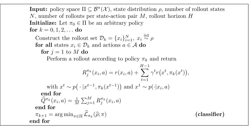
3. The DPI Algorithm
In this section, we outline the direct policy iteration (DPI) algorithm. DPI shares the
same structure as the algorithms in (Lagoudakis and Parr, 2003b) and (Fern et al., 2004). Although it can benefit from improvements in 1) selecting states for the rollout set D,
2) the criteria used to add a sample to the training set, and 3) the rollout strategy, as discussed in (Lagoudakis and Parr, 2003b) and (Dimitrakakis and Lagoudakis, 2008b), here we consider its basic form in order to ease the analysis.
DPI receives as input a policy space Π and starting from an arbitrary policy π0 ∈ Π,
at each iteration k, it computes a new policy πk+1 from πk, as the best approximation of Gπk, by solving a cost-sensitive classification problem. More formally,DPIis based on the
following loss function:
Definition 1 The loss function at iteration k for a policy π is denoted by `πk(·;π) and is
defined as
`πk(x;π) = max
a∈AQ
πk(x, a)−Qπk x, π(x), ∀x∈ X.
Given a distribution ρ over X, we define the expected error as the expectation of the loss function`πk(·;π) according to ρ,
6
Lπk(ρ;π) =
Z
X
`πk(x;π)ρ(dx) =
Z
X
h max
a∈AQ
πk(x, a)−Qπk x, π(x)
i
ρ(dx). (2)
Input: policy space Π⊆ Bπ(
X), state distributionρ, number of rollout states
N, number of rollouts per state-action pairM, rollout horizonH Initialize: Letπ0∈Π be an arbitrary policy
fork= 0,1,2, . . .do
Construct the rollout setDk={xi}Ni=1, xi
iid ∼ρ for allstatesxi ∈ Dk and actionsa∈ Ado
forj= 1 toM do
Perform a rollout according to policyπk and return
Rπk
j (xi, a) =r(xi, a) + H−1
X
t=1
γtr xt, π k(xt)
,
withxt
∼p · |xt−1, π
k(xt−1)
andx1
∼p(·|xi, a)
end for
b Qπk(x
i, a) =M1 PM
j=1R
πk j (xi, a)
end for
πk+1= arg minπ∈ΠLbπk(ρb;π) (classifier)
end for
Figure 1: The Direct Policy Iteration (DPI) algorithm.
While in (Lagoudakis and Parr, 2003b) the goal is to minimize the number of misclas-sifications using a 0/1 loss function, DPIlearns a policy trying to minimize the errorLπk.
Similar to other classification-based RL algorithms (Bagnell et al., 2003; Kakade, 2003; Fern et al., 2004; Langford and Zadrozny, 2005; Li et al., 2007),DPIdoes not focus on finding a
uniformly accurate approximation of the actions taken by the greedy policy, but rather on finding actions leading to a similar performance. This is consistent with the final objective of policy iteration, which is to obtain a policy with similar performance to an optimal policy, and not necessarily one that takes actions similar to an optimal policy.7
As illustrated in Figure 1, for each statexi∈ Dk and for each actiona∈ A, an estimate
of the action-value function of the current policy is computed through M independent rollouts. AH-horizon rollout of a policy πk for a state-action pair (xi, a) is
Rπk(x
i, a) =r(xi, a) + H−1
X
t=1
γtr xt, πk(xt)
, (3)
wherext∼p · |xt−1, π k(xt−1)
andx1∼p(·|x
i, a). The action-value function estimation is
then obtained by averaging M independent rollouts {Rπk
j (xi, a)}1≤j≤M as
b
Qπk(x
i, a) =
1
M M
X
j=1 Rπk
j (xi, a). (4)
Given the outcome of the rollouts, the empirical loss is defined as follows:
Definition 2 For any x∈ Dk, the empirical loss function at iterationk for a policy π is
b
`πk(x;π) = maxa∈AQb
πk(x, a)−
b
Qπk x, π(x),
where Qbπk(x, a) is a H-horizon rollout estimation of the action-value of πk in (x, a) as
defined by Equations 3 and 4. Similar to Definition 1, the empirical error is defined as the average over states in Dk of the empirical loss,8
b
Lπk(ρb;π) = 1
N N
X
i=1
h max
a∈AQb πk(x
i, a)−Qbπk xi, π(xi) i
,
where ρbis the empirical distribution induced by the samples in Dk.
Finally, DPI makes use of a classifier which returns a policy that minimizes the
em-pirical error Lπb k(ρb;π) over the policy space Π (see Section 6.2 for further details on the implementation of such a classifier). Note that this gap-weighted loss function has been previously used in other algorithms such as PSDP (Bagnell et al., 2003) andCPI(Kakade,
2003). Furthermore, while here we use a loss perspective, the minimization of the empirical lossLπb k(ρb;π) is equivalent to the maximization of the average Q-value and the theoretical development in the next sections would apply mostly unchanged.
4. Finite-sample Analysis of DPI
In this section, we first provide a finite-sample analysis of the error incurred at each iteration of DPIin Theorem 5, and then show how this error is propagated through the iterations
of the algorithm in Theorem 7. In the analysis, we explicitly assume that the action space contains only two actions, that is,A={a1, a2}and|A|= 2. We will discuss this assumption
and other theoretical and practical aspects of DPIin Section 6.
4.1 Error Bound at Each Iteration
Here we study the error incurred at each iterationkof theDPIalgorithm. In particular, we
compare the quality of the policyπk+1obtained by minimizing the empirical lossLπb k(ρb;·) to the policy that better approximate the greedy policyGπk among the policies in Π (i.e., the
policy minimizing the expected lossLπk(ρ;·)). Comparing the definition of the expected and empirical errors, we notice that there are three sources of error in the algorithm of Figure 1. The first one depends on the use of a finite number of samples, i.e.,N states in the rollout set, to approximate the expectation w.r.t. the distribution ρ. The second one is due to using rollouts with finite horizon H to approximate the action-value function Qπk of the
current policyπk. Finally, the third one depends on the use ofM rollouts to approximate
the action-value function of the current policy for any of the N states in the rollout set
Dk and any action in the action space A. Before stating our main result, i.e., Theorem 5, we prove bounds for the first and third sources of errors in Lemmas 3 and 4, and have a discussion on the effect of finite horizon rollouts to approximate the action-value function.
The proofs of the lemmas rely on tools from concentration inequalities of empirical processes and statistical learning theory (notably VC-bounds), and they are reported in Appendix A. Lemma 3 shows that the difference between the approximation obtained by averaging over the samples in the rollout set and the true expectation can be controlled and reduces to zero as the number of states in the rollout setN grows.
Lemma 3 Let Π be a policy space with finite VC-dimension h=V C(Π)<∞ and N >0
be the number of states in the rollout set Dk, drawn i.i.d. from the state distribution ρ at iteration k, then
PDk
sup
π∈Π
Lπk(ρb;π)− Lπk(ρ;π)
>
≤δ ,
wherePDk[·]is the probability w.r.t. the random rollout setDkconditioned on all the previous
iterations9 and = 16Qmax
q
2 N hlog
eN h + log
8 δ
.
Proof See Appendix A.
The second source of error in the algorithm of Figure 1 is due to the use of finite horizon rollout estimates of the action-value function on the states in the rollout set. We define the true action-value for a state-action pair (x, a) with a finite horizon H as
Qπk
H(x, a) =E
"
r(x, a) +
H−1
X
t=1
γtr xt, πk(xt)
#
.
It is easy to see that theH-horizon rollout estimates are stochastic estimations ofQπk
H(x, a)
which in turn satisfy
|Qπk(x, a)−Qπk
H(x, a)|=
E " ∞ X
t=H
γtr xt, πk(xt)
#
≤γHQmax. (5)
In the proof of the main theorem we also need to bound the difference between the action values (of the N states in the rollout set Dk and all the actions in the action space A) estimated with M rollouts and their true values. We thus report the following lemma to bound this source of error.
Lemma 4 LetΠbe a policy space with finite VC-dimensionh=V C(Π)<∞andx1, . . . , xN
be an arbitrary sequence of states. In each state we simulate M independent truncated roll-outs, then
PDk
sup π∈Π 1 N N X i=1 1 M M X j=1 Rπk
j (xi, π(xi))−
1
N N
X
i=1 Qπk
H(xi, π(xi))
>
≤δ ,
with = 8(1−γH)Q max
q
2
M N hlog eM N
h + log 8 δ
.
9. More precisely, the conditioning is w.r.t. all the rollout setsD0,D1, . . . ,Dk−1, which define all the policies
Proof See Appendix A.
We are now ready to prove the main result of this section. We show a high probability bound onLπk(ρ;πk+1), the expected error at any iterationkof the DPIalgorithm.
Theorem 5 Let Π be a policy space with finite VC-dimension h = V C(Π) < ∞ and ρ
be a distribution over the state space X. Let N be the number of states in Dk drawn i.i.d. from ρ at each iteration, H be the horizon of the rollouts, and M be the number of rollouts per state-action pair used in the estimation of the action-value functions. Let
πk+1 = arg minπ∈ΠLπb k(ρb;π) be the policy computed at the k-th iteration of DPI. Then, for
anyδ >0, we have
Lπk(ρ;πk+1)≤ inf
π∈ΠLπk(ρ;π) + 2(1+2+γ HQ
max), (6)
with probability1−δ, where
1= 16Qmax
s 2
N
hlogeN
h + log
32
δ
, 2= 8(1−γH)Qmax
s 2
M N
hlogeM N
h + log
32
δ
.
Remark (dependency on M and N). The bound in Equation 6 can be decomposed into an approximation error (infπ∈ΠLπk(ρ;π)) and an estimation error consisting of three
terms 1, 2, and γHQmax. This is similar to generalization bounds in classification, where
the approximation error is the distance between the target function (here the greedy policy w.r.t. πk) and the function space Π. The first estimation term,1, grows with the capacity
of Π, measured by its VC-dimension h, and decreases with the number of sampled states
N. Thus in order to avoid overfitting, we should haveN h. The second estimation term,
2, comes from the error in the estimation of the action-values due to the finite number of rolloutsM. It is important to note the nice rate of 1/√M N instead of 1/√M. This is due to the fact that we do not need a uniformly good estimation of the action-value function at all sampled states, but only an averaged estimation of those values at the sampled points. An important consequence of this is that the algorithm works perfectly well if we consider only M = 1 rollout per state-action. Therefore, given a fixed budget (number of rollouts per iteration) and a fixed rollout horizon H, the best allocation of M and N would be to choose M = 1 and sample as many states as possible, thus, reducing the risk of overfitting. The third estimation term, γHQ
max, is due to the fact that we consider a finite horizon H
for the rollouts. This term decreases exponentially fast as the rollout horizonH grows.
Remark (choice of the parameters). In Remark 1, we considered the tradeoff between the number of states, N, and the number of rollouts at each state-action pair, M, when a finite budget (number of rollouts per iteration) is given. It is also interesting to analyze the tradeoff with the rollout horizon, H, when the number of interactions with the generative model is fixed to a maximum valueS =N×M×H. The termγH decreases exponentially
a large number of states, while the rollouts may have a fairly short horizon. Nonetheless, it is clear from the value of H that the discount factor is critical, and when it approaches 1 the horizon increases correspondingly.
Remark (comparison with other classification-based methods). The performance of classification-based methods have been analyzed before by Fern et al. (2006) and Dimi-trakakis and Lagoudakis (2008a). As discussed in the Introduction, the bound reported in Theorem 5 forDPIimproves existing results over multiple dimensions. Using a regret-based
loss function allows DPI to remove the inverse dependency on the smallest gap appearing
in the analysis by Fern et al. (2006). Furthermore, this also allows us to drop the Lipschitz and the separability assumptions employed by Dimitrakakis and Lagoudakis (2008a) and extend the result to any sampling strategy ρ. In this sense, Theorem 5 provides a stronger and more general guarantee on the performance of DPI, where the only constraint is relative
to using a policy space with finite VC-dimension, conditioned enjoyed by many standard classifiers (e.g., linear separators, neural networks).
Proof [Theorem 5] Let a+(x) = arg max
a∈AQπk(x, a) be the greedy action in state x.10
We prove the following series of inequalities:
Lπk(ρ;πk+1) (a)
≤ Lπk(ρb;πk+1) +1 w.p. 1−δ
0
= 1
N N
X
i=1
h
Qπk(x
i, a+)−Qπk xi, πk+1(xi)
i +1
(b) ≤ N1
N
X
i=1
h
Qπk(x
i, a+)−QπHk xi, πk+1(xi)
i
+1+γHQmax w.p. 1−δ0 (c)
≤ 1 N
N
X
i=1
h
Qπk(x
i, a+)−Qbπk xi, πk+1(xi) i
+1+2+γHQmax w.p. 1−2δ0
(d) ≤ N1
N
X
i=1
h
Qπk(x
i, a+)−Qbπk xi, π+(xi) i
+1+2+γHQmax (e)
≤ 1 N
N
X
i=1
h
Qπk(x
i, a+)−QHπk xi, π+(xi)
i
+1+ 22+γHQmax w.p. 1−3δ0
(f) ≤ N1
N
X
i=1
h
Qπk(x
i, a+)−Qπk xi, π+(xi)
i
+1+ 2(2+γHQmax) w.p. 1−3δ0
=Lπk(ρb;π+) +
1+ 2(2+γHQmax) (g)
≤ Lπk(ρ;π
+) + 2(
1+2+γHQmax) w.p. 1−4δ0
= inf
π0∈ΠLπk(ρ;π
0) + 2(
1+2+γHQmax).
The statement of the theorem is obtained by settingδ0 =δ/4.
(a)It is an immediate application of Lemma 3, bounding the difference betweenLπk(ρ;π) and Lπk(ρb;π) for any policy π∈Π.
(b) We use the inequality in Equation 5.
(c)Here we introduce the estimated action-value function Qbπk by bounding
sup
π∈Π
" 1
N N
X
i=1
b
Qπk x
i, π(xi)
− 1 N
N
X
i=1 Qπk
H xi, π(xi)
#
,
i.e., the maximum over all the policies in the policy space11 of the difference between the
true action-value function with horizonH and its rollout estimates averaged over the states in the rollout set Dk={xi}N
i=1. We bound this term using the result of Lemma 4.
(d) From the definition ofπk+1 in theDPIalgorithm (see Figure 1), we have
πk+1 = arg min π∈Π
b
Lπk(ρb;π) = arg max
π∈Π
1
N N
X
i=1
b
Qπk x
i, π(xi)
,
thus,−1 N
PN
i=1Qbπk xi, πk+1(xi)
can be maximized by replacingπk+1with any other policy,
particularly with
π+= arg inf
π0∈Π Z
X
max
a∈AQ
πk(x, a)−Qπk x, π0(x)
ρ(dx).
(e)-(f )-(g)The final result follows by the same arguments in steps (a), (b), and (c) but in reversed order.
4.2 Error Propagation
In this section, we first show how the expected error is propagated through the iterations of DPI. We then analyze the error between the value function of the policy obtained by DPI after K iterations and the optimal value function. Unlike the per-iteration analysis,
in the propagation we consider the general case where the error is evaluated according to a
testing distributionµ which may differ from the sampling distribution ρ used to construct the rollout setsDk over iterations.
Before stating the main result, we define the inherent greedy error of a policy space Π.
Definition 6 We define the inherent greedy error of a policy space Π⊆ Bπ(X) as
d(Π,GΠ) = sup
π∈Π
inf
π0∈ΠLπ(ρ;π
0).
The inherent greedy error is the worst expected error that a error-minimizing policy
π0 ∈ Π can incur in approximating the greedy policy Gπ, for any policy π ∈ Π. This measures how well Π is able to approximate policies that are greedy w.r.t. any policy in Π.
11. The supremum over all the policies in the policy space Π is due to the fact thatπk+1is a random object,
In order to simplify the notation, we introduce Pπ as the transition kernel for policy π,
i.e., Pπ(dy|x) = p dy|x, π(x)
. We define the right-linear operator, Pπ·, which maps any V ∈ BV(X;V
max) to (PπV)(x) =
R
V(y)Pπ(dy|x), i.e., the expected value of V w.r.t. the
next states achieved by following policyπ in statex. From the definitions of `πk, T
π, and T, we have `
πk(πk+1) = TV
πk− Tπk+1Vπk. We
deduce the following pointwise inequalities:
Vπk−Vπk+1 =TπkVπk− Tπk+1Vπk +Tπk+1Vπk − Tπk+1Vπk+1
≤`πk(πk+1) +γP
πk+1(Vπk−Vπk+1), (7)
which gives us Vπk −Vπk+1 ≤ (I −γPπk+1)−1`
πk(πk+1). Since TV
πk ≥ Tπ∗Vπk, we also
have
V∗−Vπk+1 =Tπ∗V∗− TVπk+TVπk− Tπk+1Vπk+Tπk+1Vπk− Tπk+1Vπk+1
≤γP∗(V∗−Vπk) +`
πk(πk+1) +γP
πk+1(Vπk−Vπk+1),
whereP∗ =Pπ∗. Using Equation 7 this yields to
V∗−Vπk+1 ≤γP∗(V∗−Vπk) +γPπk+1(I −γPπk+1)−1+I`
πk(πk+1)
=γP∗(V∗−Vπk) + (I−γPπk+1)−1`
πk(πk+1).
Finally, by defining the operator Ek= (I−γPπk+1)−1, which is well defined sincePπk+1
is a stochastic kernel and γ <1, and by induction, we obtain
V∗−VπK ≤(γP∗)K(V∗−Vπ0) +
K−1
X
k=0
(γP∗)K−k−1Ek`πk(πk+1). (8)
Equation 8 shows how the error at each iterationkofDPI,`πk(πk+1), is propagated through
the iterations and appears in the final error of the algorithm: V∗−VπK. In particular,
the previous equation reveals the final performance loss in a state x is influenced by all the iterations where the losses in different states are combined and weighted according to the distribution obtained as the combination of the P∗ and Ek operators. Since we
are interested in bounding the final error in µ-norm, which might be different from the sampling distribution ρ, we need to state some assumptions. We first introduce the left-linear operator of the kernel Pπ as ·Pπ such that (µPπ)(dy) = R
Pπ(dy|x)µ(dx) for any
distribution µ over X. In words, µPπ correspond to the distribution over states obtained
by starting from a random state drawn fromµ and then taking the action suggested byπ.
Assumption 1 For any policy π ∈ Bπ(X) and any non-negative integers s and t, there
exists a constant Cµ,ρ(s, t)<∞ such that µ(P∗)s(Pπ)t≤Cµ,ρ(s, t)ρ.12 We assume that the
cumulative coefficient Cµ,ρ= (1−γ)2P∞s=0
P∞
t=0γs+tCµ,ρ(s, t) is bounded, i.e., Cµ,ρ<∞. Assumption 2 For any x ∈ X and any a∈ A, there exist a constant Cρ <∞ such that p(·|x, a)≤Cρρ(·).
12. Given two distributionsP andQonX and a real constantc >0,P≤cQis equivalent to the condition
Note that concentrability coefficients similar to Cµ,ρ and Cρ were previously used in
the Lp-analysis of fitted value iteration (Munos, 2007; Munos and Szepesv´ari, 2008) and
approximate policy iteration (Antos et al., 2008). See also Farahmand et al. (2010) for a more refined analysis. We now state our main result.
Theorem 7 Let Π be a policy space with finite VC-dimension h and πK be the policy
generated by DPI after K iterations. LetM be the number of rollouts per state-action and N be the number of samples drawn i.i.d. from a distribution ρ over X at each iteration of
DPI. Then, for any δ >0, we have
||V∗−VπK|| 1,µ≤
Cµ,ρ
(1−γ)2
h
d(Π,GΠ) + 2(1+2+γHQmax)i+ 2γ
KRmax
1−γ , (under Asm. 1)
||V∗−VπK||
∞≤ Cρ
(1−γ)2
h
d(Π,GΠ) + 2(1+2+γHQmax)
i + 2γ
KRmax
1−γ , (under Asm. 2)
with probability1−δ, where
1= 16Qmax s
2
N
hlogeN
h + log
32K δ
and 2= 8(1−γH)Qmax s
2
M N
hlogeM N
h + log
32K δ
.
Remark (sample complexity). From the previous bound on the performance loss of DPI after K iterations, we can deduce the full sample complexity of the algorithm.
Let be the desired performance loss when stopping the algorithm, from the remarks of Theorem 5 and the previous bound, we see that a logarithmic number of iterations
K() =O(log(1/)/(1−γ)) is enough to reduce the last term toO(). On the other hand, for the leading term, if we ignore the inherent greedy error, which is a constant bias term and setM = 1, the number of samples required per iteration is13
N() =O
hQ2 max 2(1−γ)4
,
which amounts to a total of N()K() samples across iterations. In this case, the final bound is ||V∗ −VπK||
1,µ ≤ Cµ,ρ(d(Π,GΠ) +). As discussed in the Introduction and
analyzed in details by Ghavamzadeh and Lazaric (2012), this result is competitive with other approximate policy iteration (API) schemes such as conservative policy iteration (CPI).
Remark (comparison with other value-function-based API). Although a direct and detailed comparison between classification-based and value-function-based approaches to API is not straightforward, it is interesting to discuss their similarities and differences.
For value-function-based API, we refer to, e.g., LSPI (Lagoudakis and Parr, 2003a) and
in particular the theoretical analysis developed by Lazaric et al. (2012) (see Theorem 8 therein). Although here we analyzedDPIfor a generic policy space Π and the performance is
evaluated inL1-norm, whileLSPIexplicitly relies on linear spaces and the norm isL2,
high-level similarities and differences can be remarked in the performance of the two methods. The structure of the bounds is similar for both methods and notably the dependency on
the number of samples N, number of iterationsK, and discount factor γ is the same. The major difference lays in the concentrability coefficients and in the shape of the approximation error. While assumption on the coefficients Cµ,ρ(s, t) forDPI is less tight since it requires
to bound the distributionµ(P∗)s(Pπ)tinstead of the distributionµPπ1. . . Pπm obtained for
any possible sequence of policies, the final coefficientsCµ,ρare more involved and difficult to
compare. On the other hand, it is interesting to notice that the approximation errors share the same structure. In fact, they both consider the worst approximation error w.r.t. all the possible approximation problems that could be faced across iterations. While this reveals the importance of the choice of an appropriate approximation space in both cases, it also supports the claim that a classification-based method may be preferable whenever it is easier to design a set of “good” policies rather than a set of “good” value functions.
Remark (convergence). Similar to other API algorithms, Theorem 7 states that DPI
may oscillate over different policies whose performance loss in bounded. Nonetheless, de-pending on the policy space Π and the MDP at hand, in practiceDPIsometimes converges
to a fixed policy ¯π. Let D : Bπ(X) → Bπ(X) be the policy operator corresponding to
the approximation performed by DPI at each iteration (i.e., constructing rollouts from a
given policy and solving the classification problem), thenDPIcan be written compactly as πk+1 =DGπk. If DPIconverges to ¯π, then the joint operatorDG admits ¯π as a fixed point,
i.e., ¯π = DG¯π and the per-iteration error `πk(πk+1), which is propagated in the analysis
of Theorem 7, converges to `π¯(¯π). In this case, the performance loss of ¯π can be directly
studied as a function of the error Lπ¯(ρ,π¯) as (see Munos, 2007, Section 5.2 for a similar
argument for approximate value iteration)
V∗−Vπ¯ =Tπ∗V∗
− TVπ¯+TVπ¯−V¯π ≤ Tπ∗V∗
− Tπ∗Vπ¯+TVπ¯−V¯π
=γP∗(V∗− Tπ∗V¯π) +TVπ¯− Tπ¯Vπ¯.
Using the definition of `¯π(¯π) we obtain the following component-wise performance loss
V∗−V¯π ≤(I−γP∗)−1`π¯(¯π).
Finally, integrating on both sides w.r.t. the measureµwe have
||V∗−V¯π||1,µ ≤ C∗
µ,ρ
1−γ
h inf
π0∈ΠL¯π(ρ;π
0) + 2(
1+2+γHQmax)
i
,
where the concentrability coefficient Cµ,ρ∗ is such that µP∞
t=0(γP
∗)t ≤ C∗
µ,ρρ. Unlike the
coefficients introduced in Assumption 1, Cµ,ρ∗ only involves the optimal policy and notably the discounted stationary distribution of π∗. This term coincides with the coefficient
ap-pearing in the performance of CPI and it can be made small by appropriately choosing
factor reduces by a factor of 1/(1−γ) and the approximation error appearing in the final bound no longer depends on the inherent greedy error. It only depends on the loss of the policy that better approximatesGπ¯ in Π.
Proof [Theorem 7] We have Cµ,ρ ≤Cρ for any µ. Thus, if the L1-bound holds for any µ,
choosingµto be a Dirac at each state implies that theL∞-bound holds as well. Hence, we
only need to prove the L1-bound. By taking the absolute value point-wise in Equation 8
we obtain
|V∗−VπK| ≤(γP∗)K|V∗−Vπ0|+
K−1
X
k=0
(γP∗)K−k−1(I −γPπk+1)−1|`
πk(πk+1)|.
From the fact that |V∗−Vπ0| ≤ 2
1−γRmax1, and by integrating both sides w.r.t. µ, and
expanding (I−γPπk+1
)−1 =P∞
t=0(γPπk+1)t we have ||V∗−VπK||
1,µ ≤
2γK
1−γRmax+ K−1
X
k=0 ∞
X
t=0
γK−k−1γt
Z
X
µ(P∗)K−k−1(Pπk+1 )t
(dx)|`πk(dx;πk+1)|.
The integral in the second term corresponds to the expected loss w.r.t. to the distribution over states obtained by starting from µ and then applying K−k−1 steps of the optimal policy and t steps of policy πk+1. This term does not correspond to what is actually
minimized by DPIat each iteration, and thus, we need to apply Assumption 1 and obtain
||V∗−VπK|| 1,µ≤
2γK
1−γRmax+ K−1
X
k=0 ∞
X
t=0
γK−k−1γtCµ,ρ(K−k−1, t)Lπk(ρ;πk+1).
From the definition of Cµ,ρ we obtain
||V∗−VπK|| 1,µ ≤
2γK
1−γRmax+ Cµ,ρ
(1−γ)2 0≤k≤Kmax Lπk(ρ;πk+1).
The claim follows from bounding Lπk(ρ;πk+1) using Theorem 5 with a union bound
argu-ment over the K iterations and from the definition of the inherent greedy error.
5. Approximation Error
In Section 4.2, we analyzed how the expected error at each iterationkof DPI,Lπk(ρ;πk+1),
Definition 8 A sequence of policy spaces {Πn} is a universal family of policy spaces, if there exists a sequence of real numbers {βn} with lim
n→∞βn = 0, such that for any n > 0,
Πn is induced by a partition Pn = {Xi}iS=1n over the state space X (i.e., for each Sn-tuple
(b1, . . . , bSn) withbi ∈ {0,1}, there exists a policy π ∈Πn such thatπ(x) =bi for all x∈ Xi
and for all i∈ {1, . . . , Sn}) in such a way that
max
1≤i≤Sn
max
x,y∈Xi||
x−y|| ≤βn.
This definition requires that for any n > 0, Πn is the space of policies induced by a
partitionPn and the diameters of the elementsXi of this partition shrink to zero asngoes
to infinity. The main property of such a sequence of spaces is that any fixed policy π can be approximated arbitrary well by policies of Πnwhen n→ ∞. Although other definitions
of universality could be used, Definition 8 seems natural and it is satisfied by widely-used classifiers such ask-nearest neighbor, uniform grid, and histogram.
In the next section, we first show that the universality of a policy space (Definition 8) does not guarantee that d(Πn,GΠn) converges to zero in a general MDP. In particular,
we present an MDP in which d(Πn,GΠn) is constant (does not depend on n) even when {Πn}is a universal family of classifiers. We then prove that in Lipschitz MDPs,d(Πn,GΠn)
converges to zero for a universal family of policy spaces.
5.1 Counterexample
In this section, we illustrate a simple example in which d(Πn,GΠn) does not go to zero,
even when {Πn} is a universal family of classifiers. We consider an MDP with state space
X = [0,1], action spaceA={0,1}, and the following transitions and rewards
xt+1=
(
min(xt+ 0.5,1) if a= 1,
xt otherwise,
r(x, a) =
0 if x= 1, R1 else if a= 1, R0 otherwise,
where (1−γ2)R1< R0 < R1. (9)
We consider the policy space Πn of piecewise constant policies obtained by uniformly
partitioning the state spaceX intonintervals. This family of policy spaces is universal. The inherent greedy error of Πn,d(Πn,GΠn), can be decomposed into the sum of the expected
errors at each interval
d(Πn,GΠn) = sup π∈Πn
inf
π0∈Π
n
n
X
i=1 L(i)
π (ρ;π0),
where L(πi)(ρ;π0) is the same as Lπ(ρ;π0), but with the integral limited to thei-th interval
instead of the entire state space X. In the following we show that for the MDP and the universal class of policies considered here,d(Πn,GΠn) does not converge to zero asngrows.
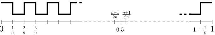
Let n be odd andπ ∈Πn be one in odd and zero in even intervals (see Figure 2). For
1−1
n
0
1n n2 3n
n+1 2n n−1
2n
0.5
1
Figure 2: The policy used in the counterexample. It is one in odd and zero in even intervals. Note that the number of intervals,n, is assumed to be odd.
out of bound in one step by taking action 1. Thus, given the assumption of Equation 9, it can be shown that for any x belonging to the intervalsi≥ n+1
2 (the interval containing
0.5 and above), (Gπ)(x) = 0. This means that there exists a policy π0 ∈ Πn such that L(πi)(ρ;π0) = 0 for all the intervals i≥ n+12 . However, Gπ does not remain constant in the
intervalsi≤ n−1
2 , and changes its value in the middle of the interval. Using Equation 9, we
can show that
inf
π0∈Π
n
n
X
i=1 L(i)
π (ρ;π 0
) =C1 + 1 1−γ
n−1 8n ≥
C
16
1 + 1
1−γ
,
whereC = min
(1−γ)(R1−R0), R0−(1−γ2)R1 . This means that for any odd n, it is
always possible to find a policyπ ∈Πn such that infπ0∈Π
nLπ(ρ;π
0) is lower bounded by a
constant independent ofn, and thus, limn→∞d(Πn,GΠn)6= 0.
5.2 Lipschitz MDPs
In this section, we prove that for Lipschitz MDPs,d(Πn,GΠn) goes to zero when{Πn} is a
universal family of classifiers. We start by defining a Lipschitz MDP.
Definition 9 A MDP is Lipschitz if both its transition probability and reward functions are Lipschitz, i.e., ∀(B, x, x0, a)∈ B(X)× X × X × A
|r(x, a)−r(x0, a)| ≤Lrkx−x0k, |p(B|x, a)−p(B|x0, a)| ≤Lpkx−x0k,
with Lr and Lp being the Lipschitz constants of the transitions and reward, respectively.
An important property of Lipschitz MDPs is that for any functionQ∈ BQ(X ×A;Q max),
the function obtained by applying the Bellman operatorTπ toQ(·, a), (TπQ)(·, a), is
Lip-schitz with constant L= (Lr+γQmaxLp), for any action a∈ A. In fact, for any policy π,
any actiona∈ Aand any pair x, x0∈ X we have
(TπQ)(x, a)−(TπQ)(x0 , a)
=r(x, a) +γ
Z
X
p(dy|x, a)Qπ(y, π(y))−r(x0, a)−γ
Z
X
p(dy|x0, a)Qπ(y, π(y))
≤Lr||x−x0||+γ
Z
X
p(dy|x, a)−p(dy|x0, a)
Q(y, π(y))
As a result, the function Qπ(·, a), which is the unique fixed point of the Bellman operator Tπ, is Lipschitz with constantL, for any policyπ ∈ Bπ(X) and any action a∈ A.
Theorem 10 Let M be a Lipschitz MDP with |A|= 2 and {Πn} be a universal family of policy spaces (Definition 8). Then limn→∞d(Πn,GΠn) = 0.
Proof
d(Πn,GΠn) = sup π∈Πn
inf
π0∈Π
n
Z
X
`π(x;π0)ρ(dx)
(a)
= sup
π∈Πn
inf
π0∈Π
n
Z
XI
(Gπ)(x)6=π0(x) ∆π(x)ρ(dx)
(b)
= sup
π∈Πn
inf
π0∈Π
n
Sn
X
i=1
Z
Xi
I(Gπ)(x)6=π0(x) ∆π(x)ρ(dx)
(c)
= sup
π∈Πn
Sn
X
i=1
min
a∈A
Z
Xi
I{(Gπ)(x)6=a}∆π(x)ρ(dx)
(d) ≤ sup
π∈Πn
Sn
X
i=1
min
a∈A
Z
Xi
I{(Gπ)(x)6=a}2L inf
y:∆π(y)=0kx−ykρ(dx) (e)
≤ 2L sup
π∈Πn
Sn
X
i=1
min
a∈A
Z
Xi
I{(Gπ)(x)=6 a}βnρ(dx)
(f) ≤ 2Lβn
Sn
X
i=1
Z
Xi
ρ(dx) = 2Lβn.
(a)We rewrite Definition 6, where ∆π(x) = max
a∈AQπ(x, a)−mina0∈A(x, a0) is the regret of choosing the wrong action in state x.
(b) Since Πn contains piecewise constants policies induced by the partitionPn={Xi}, we
split the integral as the sum over the regions.
(c) Since the policies in Πn can take any action in each possible region, the policy π0
minimizing the loss is the one which takes the best action in each region.
(d) Since M is Lipschitz, both maxa∈AQπ(·, a) and mina0∈AQπ(·, a0) are Lipschitz, and thus, ∆π(·) is 2L-Lipschitz. Furthermore, ∆π is zero in all the states in which the policy Gπ changes (see Figure 3). Thus, for any state x the value ∆π(x) can be bounded using
the Lipschitz property by takingy as the closest state to xin which ∆π(y) = 0.
(e)IfGπis constant in a regionXi, the integral can be made zero by settingato the greedy action (thus making I{(Gπ)(x)=6 a} = 0 for any x ∈ Xi). Otherwise, if Gπ changes in a
statey∈ Xi, then ∆π(y) = 0 and we can replace||x−y||by the diameter of the region which
is bounded byβnaccording to the definition of the universal family of spaces (Definition 8). (f ) We simply takeI{(Gπ)(x)6=a}= 1 in each region.
a2
Qπ(x, a
2)
Qπ(x, a
1)
0 0.2 0.4 0.6 0.8 1
∆π(x)
a1
(Gπ)(x)
Figure 3: This figure is used as an illustrative example in the proof of Theorem 10. It shows the action-value function of a Lipschitz MDP for a policyπ,Qπ(·, a1) and Qπ(·, a
2) (top), the corresponding greedy policy Gπ (middle), and the regret of
selecting the wrong action, ∆π, (bottom).
Theorem 10 together with the counter-example in Section 5.1 show that the assumption on the policy space is not enough to guarantee a small approximation error and additional assumptions on the smoothness of the MDP (e.g., Lipschitz condition) must be satisfied.
5.3 Consistency of DPI
A highly desirable property of any learning algorithm is consistency, i.e., as the number of samples grows to infinity, the error of the algorithm converges to zero. It can be seen that as the number of samplesN and the rollout horizon H grow in Theorem 5, 1 and 2 become
arbitrarily small, and thus, the expected error at each iteration, Lπk(ρ;πk+1), is bounded
by the inherent greedy error d(Πn,GΠn). We can conclude from the results of this section
that DPIis not consistent in general, but it is consistent for the class of Lipschitz MDPs,
when a universal family of policy spaces is used andntends to infinite andd(Πn,GΠn) can
be reduced to zero. However, it is important to note that as we increase the index n to reduce the inherent greedy error, the capacity of the policy space Π (its VC-dimensionh is indeed a function of n) grows as well, and thus, the error terms 1 and 2 may no longer
decrease to zero. As a result, to guarantee consistency, we need to link the growth of the policy space Π to the number of samplesN, so that asN goes to infinity, the capacity of Π grows at a lower rate and the estimation errors still vanish. More formally, for any number of samplesN, we choose an indexnso that the corresponding space Π has a VC-dimension
h(N) such that limN→∞h(N)/N = 0. We deduce the following result.
Assumption 1 or 2, DPIis consistent:
lim
N, H, K→ ∞
δ→0
VπK =V∗ , w.p. 1.
Notice that the result in the previous corollary is possible because the Assumption 1 already covers any policy π inBπ(X) and is not limited to the policies in Π
n.
6. Extension to Multiple Actions
The analysis of Sections 4 and 5 are for the case that the action space contains only two actions. In Section 6.1 we extend the previous theoretical analysis to the general case of an action space with |A| > 2. While the theoretical analysis is completely independent from the specific algorithm used to solve the empirical error minimization problem (see
DPIalgorithm of Figure 1), in Section 6.2 we discuss which algorithms could be employed
to solve this problem in the case of multiple actions.
6.1 Theoretical Analysis
From the theoretical point of view, the extension of the previous results to multiple actions is straightforward. The definitions of loss and error functions do not change and we just need to use an alternative complexity measure for multi-class classification. We rely on the following definitions from (Ben-David et al., 1995).
Definition 12 Let Π ⊆ Bπ(X) be a set of deterministic policies and Ψ =
ψ : A →
{0,1,∗} be a set of mappings from the action space to the set {0,1,∗}. A finite set of
N states XN = {xi}Ni=1 ⊆ X is Ψ-shattered by Π if there exists a vector of mappings ψN = ψ(1), . . . , ψ(N)>
∈ ΨN such that for any vector v ∈ {0,1}N, there exist a policy π ∈ Π such that ψ(i)◦π(x
i) = vi, 1 ≤ i ≤ N. The Ψ-dimension of Π is the maximal
cardinality of a subset of X, Ψ-shattered by Π.
Definition 13 Let Π ⊆ Bπ(X) be a set of deterministic policies and Ψ =
ψk,l : A → {0,1,∗}, 1≤k6=l≤L be a set of possible mappings such that
ψk,l(a) =
1 if a=k,
0 if a=l, ∗ otherwise,
then the Natarajan dimension of Π, N-dim(Π), is theΨ-dimension of Π.
By using a policy space with finite Natarajan dimension, we derive the following corollary to Theorem 5.
Corollary 14 Let Π ⊆ Bπ(X) be a policy space with finite Natarajan dimension h =
DPIin the estimation of the action-value functions. Letπk+1= arg minπ∈ΠLπb k(ρb;π)be the
policy computed at the k-th iteration of DPI. Then, for any δ >0, we have
Lπk(ρ;πk+1)≤ inf
π∈ΠLπk(ρ;π) + 2(1+2+γ
HQmax), (10)
with probability1−δ, where
1 = 16Qmax
s 2
N
hlog|A|e(N+ 1)
2
h + log
32
δ
, 2= (1−γH)Qmax
r 2
M N log
4|A| δ .
Proof In order to prove this corollary we just need a minor change in Lemma 3, which now becomes a concentration of measures inequality for a space of multi-class classifiers Π with finite Natarajan dimension. By using similar steps as in the proof of Lemma 3 and by recalling the Sauer’s lemma for finite Natarajan dimension spaces (Ben-David et al., 1995), we obtain
P
sup
π∈Π
Lπk(ρb;π)− Lπk(ρ;π)
>
≤δ ,
with = 16Qmax
r
2 N
hlog|A|e(Nh+1)2 + log8 δ
. The rest of the proof is exactly the same
as in Theorem 5.
Similarly, the consistency analysis in case of Lipschitz MDPs remains mostly unaffected by the introduction of multiple actions.
Corollary 15 Let {Πn} be a universal family of policy spaces (Definition 8), and Mbe a Lipschitz MDP (Definition 9). Then limn→∞d(Πn,GΠn) = 0.
Proof The critical part in the proof is the definition of the gap function, which now compares the performance of the greedy action to the performance of the action chosen by the policyπ0:
∆π,π0(x) = max
a∈AQ π(x, a)
−Qπ x, π0(x)
.
Note that ∆π,π0(·) is no longer a Lipschitz function because it is a function ofxthrough the
policy π0. However, ∆π,π0(x) is Lipschitz in each region Xi, i = 1. . . , S
n, because in each
regionXi, by the definition of the policy space, π0 is forced to be constant. Therefore, in a
regionXi in which π0(x) =a, ∀x∈ Xi, ∆π,π0(x) may be written as
∆π,π0(x) = ∆π,a(x) = max
a0∈AQ
π(x, a0
The proof here is exactly the same as in Theorem 10 up to step(c), and then we have
d(Πn,GΠn) = sup π∈Πn
inf
π0∈Π
n
Z
X
`π(x;π0)ρ(dx)
= sup
π∈Πn
inf
π0∈Π
n
Z
X
I(Gπ)(x)6=π0(x) ∆π,π
0
(x)ρ(dx)
= sup
π∈Πn
inf
π0∈Π
n Sn X i=1 Z Xi
I(Gπ)(x)6=π0(x) ∆π,π
0
(x)ρ(dx)
= sup
π∈Πn
Sn X i=1 min a∈A Z Xi
I{(Gπ)(x)6=a}∆π,a(x)ρ(dx)
≤ sup
π∈Πn
Sn X i=1 min a∈A Z Xi
∆π,a(x)ρ(dx). (11)
If the greedy action does not change in a region Xi, i.e., ∀x ∈ Xi, (Gπ)(x) = a0, for an actiona0 ∈ A, then the minimizing policy π0 must select actiona0 inXi, and thus, the loss
will be zero inXi. Now let assume that the greedy action changes at a state y∈ Xi and the actionbi ∈arg maxa∈AQπ(y, a). In this case, we have
min
a∈A
Z
Xi
∆π,a(x)ρ(dx)≤ Z
Xi
∆π,bi(x)ρ(dx)≤
Z
Xi
∆π,bi(y) + 2Lkx−yk
ρ(dx),
since the function x 7→ ∆π,bi(x) is 2L-Lipschitz. Now since ∆π,bi(y) = 0, we deduce from
Equation 11 that
d(Πn,GΠn)≤ sup π∈Πn
Sn
X
i=1
Z
Xi
2L||x−y||ρ(dx)≤ sup
π∈Πn
Sn
X
i=1
Z
Xi
2Lβnρ(dx) = 2Lβn.
The claim follows using the definition of the universal family of policy spaces.
6.2 Algorithmic Approaches
From an algorithmic point of view, the most critical part of the DPIalgorithm (Figure 1)
is minimizing the empirical error, which in the case of|A|>2 is in the following form:
min
π∈ΠLπb k(ρb;π) = minπ∈Π
1 N N X i=1 h max
a∈AQb πk(x
i, a)−Qbπk xi, π(xi) i = min π∈Π N X i=1 I arg max
a∈AQb πk(x
i, a)6=π(xi)
h
max
a∈AQb πk(x
i, a)−Qbπk xi, π(xi) i
.
taken by policy π. It is important to note that here the main difference with regression is that the goal is not to have a good approximation of the action-value function over the entire state and action space. The main objective is to have a good enough estimate of the action-value function to find the greedy action in each state. A thorough discussion on the possible approaches to MCCS classification is out of the scope of this paper, and thus, we only mention a few recent methods that could be suitable for our problem. The reduction methods proposed by Beygelzimer et al. (2005, 2009) reduce the MCCS classification prob-lem to a series of weighted binary classification probprob-lems (which in turn can be reduced to binary classification as in Zadrozny et al. 2003), whose solutions can be combined to obtain a multi-class classifier. The resulting multi-class classifier is guaranteed to have a performance which is upper-bounded by the performance of each binary classifier used in solving the weighted binary problems. Another common approach to MCCS classification is to use boosting-based methods (e.g., Lozano and Abe 2008; Busa-Fekete and K´egl 2010). A recent regression-based approach has been proposed by Tu and Lin (2010), which reduces the MCCS classification to a one-sided regression problem that can be effectively solved by a variant of SVM. Finally, a theoretical analysis of the risk bound for MCCS classification is derived by ´Avila Pires et al. (2013), while Mineiro (2010) studies error bounds in the case of a reduction from MCCS to regression.
7. Conclusions
In this paper, we presented a variant of the classification-based approach to approximate policy iteration (API) called direct policy iteration (DPI) and provided its finite-sample
performance bounds. To the best of our knowledge, this is the first complete finite-sample analysis for this class of API algorithms. The main difference of DPI with the existing
classification-based API algorithms (Lagoudakis and Parr, 2003b; Fern et al., 2004) is in
weighting each classification error by its actual regret, i.e., the difference between the action-values of the greedy action and the action selected by DPI. Our results extend the only
theoretical analysis of a classification-basedAPI algorithm (Fern et al., 2006) by1)having
a performance bound for the fullAPI algorithm instead of being limited to one step policy
update,2)considering any policy space instead of finite class of policies, and 3)deriving a bound which does not depend on the Q-advantage, i.e., the minimum Q-value gap between a greedy and a sub-greedy action over the state space, which can be arbitrarily small in a large class of MDPs. Note that the final bound in (Fern et al., 2006) depends inversely on the Q-advantage. We also analyzed the consistency of DPIand showed that although it is
not consistent in general, it is consistent for the class of Lipschitz MDPs. This is similar to the consistency results for fitted value iteration in (Munos and Szepesv´ari, 2008).
One of the main motivations of this work is to have a better understanding of how the classification-based API methods can be compared with their widely-used
regression-based counterparts. It is interesting to note that the bound of Equation 6 shares the same structure as the error bounds for the API algorithm in (Antos et al., 2008) and the
which mainly depends on the number of samples and rollouts. The difference between the approximation error of the two approaches depends on how well the hypothesis space fits the MDP at hand. This confirms the intuition that whenever the policies generated by policy iteration are easier to represent and learn than their value functions, a classification-based approach can be preferable to regression-based methods.
Possible directions for future work are:
• The classification problem: As discussed in Section 6.2 the main issue in the implemen-tation of DPIis the solution of the multi-class cost-sensitive classification problem at
each iteration. Although some existing algorithms might be applied to this problem, further investigation is needed to identify which one is better suited for DPI. In
par-ticular, the main challenge is to solve the classification problem without first solving a regression problem on the cost function which would eliminated the main advantage of classification-based approaches (i.e., no approximation of the action-value function over the whole state-action space).
• Rollout allocation: In DPI, the rollout set is build with states drawn i.i.d. from an
arbitrary distribution and the rollouts are performed the same number of times for each action in A. A significant advantage could be obtained by allocating resources (i.e., the rollouts) to regions of the state space and to actions whose action-values are more difficult to estimate. This would result in a more accurate training set for the classification problem and a better approximation of the greedy policy at each iteration. Although some preliminary results in (Dimitrakakis and Lagoudakis, 2008b) and (Gabillon et al., 2010) show encouraging results, a full analysis of what is the best allocation strategy of rollouts over the state-action space is still missing.
Acknowledgments