Convergence Analysis of Distributed Inference with
Vector-Valued Gaussian Belief Propagation
Jian Du [email protected]
Department of Electrical and Computer Engineering Carnegie Mellon University
Pittsburgh, PA 15213, USA
Shaodan Ma [email protected]
Department of Electrical and Computer Engineering University of Macau
Avenida da Universidade, Taipa, Macau
Yik-Chung Wu [email protected]
Department of Electrical and Electronic Engineering The University of Hong Kong
Pokfulam Road, Hong Kong
Soummya Kar [email protected]
Jos´e M. F. Moura [email protected]
Department of Electrical and Computer Engineering Carnegie Mellon University
Pittsburgh, PA 15213, USA
Editor:Qiang Liu
Abstract
This paper considers inference over distributed linear Gaussian models using factor graphs and Gaussian belief propagation (BP). The distributed inference algorithm involves only local computation of the information matrix and of the mean vector, and message passing between neighbors. Under broad conditions, it is shown that the message information matrix converges to a unique positive definite limit matrix for arbitrary positive semidefinite initialization, and it approaches an arbitrarily small neighborhood of this limit matrix at an exponential rate. A necessary and sufficient convergence condition for the belief mean vector to converge to the optimal centralized estimator is provided under the assumption that the message information matrix is initialized as a positive semidefinite matrix. Further, it is shown that Gaussian BP always converges when the underlying factor graph is given by the union of a forest and a single loop. The proposed convergence condition in the setup of distributed linear Gaussian models is shown to be strictly weaker than other existing convergence conditions and requirements, including the Gaussian Markov random field based walk-summability condition, and applicable to a large class of scenarios.
Keywords: Graphical Model, Large-Scale Networks, Linear Gaussian Model, Markov Random Field, Walk-summability.
c
1. Introduction
Inference based on a set of measurements from multiple agents on a distributed network is a central issue in many problems. While centralized algorithms can be used in small-scale networks, they face difficulties in large-scale networks, imposing a heavy communication burden when all the data is to be transported to and processed at a central processing unit. Dealing with highly distributed data has been recognized by the U.S. National Research Council as one of the big challenges for processing big data (National Research Council, 2013). Therefore, distributed inference techniques that only involve local communication and computation are important for problems arising in distributed networks.
In large-scale linear parameter learning with Gaussian measurements, Gaussian Belief Propagation (BP) (Weiss and Freeman, 2001a) provides an efficient distributed algorithm for computing the marginal means of the unknown parameters, and it has been adopted in a variety of topics including image interpolation (Xiong et al., 2010), distributed power system state inference (Hu et al., 2011), distributed beamforming (Ng et al., 2008), dis-tributed synchronization (Du and Wu, 2013b), fast solver for system of linear equations (Shental et al., 2008a), distributed rate control in ad-hoc networks (Zhang et al., 2010), factor analyzer network (Frey, 1999), sparse Bayesian learning (Tan and Li, 2010), inter-cell interference mitigation (Lehmann, 2012), and peer-to-peer rating in social networks (Bickson and Malkhi, 2008).
Although with great empirical success (Murphy et al., 1999), it is known that a major challenge that hinders BP is the lack of theoretical guarantees of convergence in loopy net-works (Chertkov and Chernyak, 2006; G´omez et al., 2007). Convergence of other forms of loopy BP are analyzed by Ihler et al. (2005), Mooij and Kappen (2005, 2007), Noorshams and Wainwright (2013), and Ravanbakhsh and Greiner (2015), but their analyses are not directly applicable to Gaussian BP. Sufficient convergence conditions for Gaussian BP have been developed in Weiss and Freeman (2001a); Malioutov et al. (2006); Moallemi and Roy (2009a); Su and Wu (2015) when the underlying Gaussian distribution is expressed in terms of pairwise connections between scalar variables, i.e., it is a Markov random field (MRF). However, depending on how the underlying joint Gaussian distribution is factorized, Gaus-sian BP may exhibit different convergence properties as different factorizations (different Gaussian models) lead to fundamentally different recursive update structures. In this pa-per, we study the convergence of Gaussian BP derived from the distributed linear Gaussian model. The motivation is twofold. From the factorization viewpoint, by specifically em-ploying a factorization based on the linear Gaussian model, we are able to bypass difficulties in existing convergence analyses ((Malioutov et al., 2006) and references therein) based on Gaussian Markov random field factorization. From the distributed inference viewpoint, the linear Gaussian model and associated message passing requirements for implementing the Gaussian BP readily conform to the physical network topology arising in large-scale net-works such as in (Hu et al., 2011; Ng et al., 2008; Du and Wu, 2013b; Shental et al., 2008a; Zhang et al., 2010; Frey, 1999; Tan and Li, 2010; Lehmann, 2012; Bickson and Malkhi, 2008), thus it is practically important.
arbitrary valid Gaussian model, however, it is not clear how to adapt it to the distributed and parallel inference setup. In contrast, Gaussian BP is a parallel and fully distributed method that computes the marginal means by computing only the block diagonal elements of the information matrix inverse. Though the block diagonal elements computed by Gaussian BP may not be correct, it is shown that the belief mean still converges to the correct value once Gaussian BP converges. This explains the popularity of Gaussian BP in distributed inference applications, even though its convergence properties are not fully understood.
To fill this gap, this paper studies the convergence of Gaussian BP for linear Gaussian models. Specifically, for the first time, by establishing certain contractive properties of the distributed information matrix (inverse covariance matrix) updates with respect to the Birkhoff metric, we show that, with arbitrary positive semidefinite (p.s.d.) initial message information matrix, the belief covariance for each local variable converges to a unique posi-tive definite limit, and it approaches an arbitrarily small neighborhood of this limit matrix at an exponential rate. Consequently, the recursive equation for the message mean, which depends on the information matrix, can be reduced to a linear recursive equation. Further, we derive a necessary and sufficient convergence condition for this linear recursive equation under the assumption that the initial message information matrix is p.s.d. Furthermore, we show that, when the structure of the factor graph is the union of a single loop and a forest, Gaussian BP always converges. Finally, it is demonstrated that the proposed conver-gence condition for the linear Gaussian model encompasses the walk-summable converconver-gence condition for Gaussian MRFs (Malioutov et al., 2006).
Note that there exist other distributed estimation frameworks, e.g., consensus+inn-ovations (Kar and Moura, 2013; Kar et al., 2013) and diffusion algorithms (Cattivelli and Sayed, 2010) that enable distributed estimation of parameters and processes in multi-agent networked environments. The consensus+innovation algorithms converge in mean square sense to the centralized optimal solution under the assumption of global observability of the (aggregate) sensing model and connectivity (on the average) of the inter-agent com-munication network. In particular, these algorithms allow the comcom-munication or message exchange network to be different from the physical coupling network of the field being es-timated where either networks can be arbitrarily connected with cycles. The results in Kar and Moura (2013); Kar et al. (2013) imply that the unknown field or parameter can be reconstructed completely at each agent in the network. For large-scale networks with high dimensional unknown variable, it may be impractical though to estimate all the un-knowns at every agent. Reference (Kar, 2010, section 3.4) develops approaches to address this problem, where under appropriate conditions, each agent can estimate only a subset of the unknown parameter variables. This paper studies a different distributed inference problem where each agent learns only its own unknown random variables; this leads to lower dimensional data exchanges between neighbors.
The rest of this paper is organized as follows. Section 2 presents the system model for distributed inference. Section 3 derives the vector-valued distributed inference algorithm based on Gaussian BP. Section 4 establishes convergence conditions, and Section 5 discloses the relationship between the derived results and existing convergence conditions of Gaussian BP. Finally, Section 6 presents our conclusions.
respectively. The symbolIN denotes theN×N identity matrix, andN (x|µ,R) stands for
the probability density function (PDF) of a Gaussian random vector x with mean µ and covariance matrixR. The notation ||x−y||2
W stands for (x−y)
TW(x−y). The symbol ∝represents the linear scalar relationship between two real valued functions. For Hermitian matrices X and Y, XY (XY) means thatX−Y is positive semidefinite (definite). The sets [A,B] are defined by [A,B] = {X:BXA}. The symbol Bdiag{·} stands for block diagonal matrix with elements listed inside the bracket;⊗ denotes the Kronecker product; and Xi,j denotes the component of matrix Xon the i-th row and j-th column.
2. Problem Statement and Markov Random Field
Consider a general connected network1 ofM agents, withV ={1, . . . , M}denoting the set of agents, and ENet ⊂ V × V the set of all undirected communication links in the network, i.e., if i and j can communicate or exchange information directly, (i, j) ∈ ENet. At every agentn∈ V, the local observations are given by a linear Gaussian model:
yn= X
i∈n∪I(n)
An,ixi+zn, (1)
whereI(n) denotes the set of neighbors of agentn(i.e., all agentsiwith (n, i)∈ ENet),An,i
is a known coefficient matrix with full column rank, xi is the local unknown parameter at
agentiwith dimensionNi×1 and with prior distributionxi ∼ N(xi|0,Wi) (Wi0), and
zn is the additive noise with distribution zn∼ N(zn|0,Rn), where Rn0. It is assumed
thatp(xi,xj) =p(xi)p(xj) andp(zi,zj) =p(zi)p(zj) fori6=j, and the xi’s andzj’s are
independent for all iandj. The goal is to learnxi, based on yn,p(xi), and p(zn).2
In centralized estimation, all the observations yn’s at different agents are forwarded to a central processing unit. Define vectors x, y, and z as the stacking of xn, yn, and zn in
ascending order with respect to n, respectively; then, we obtain
y=Ax+z, (2)
where A is constructed from An,i, with specific arrangement dependent on the network
topology. Assuming A is of full column rank, and since (2) is a standard linear model,
the optimal minimum mean squared error estimate bx , hxb
T 1, . . . ,bx
T M
iT
of x is given by
(Murphy, 2012)
b
x=
Z
xR p(x)p(y|x)
p(x)p(y|x) dxdx= W
−1+ATR−1A−1
ATR−1y, (3)
whereWandRare block diagonal matrices containingWi andRi as their diagonal blocks,
respectively. Although well-established, centralized estimation in large-scale networks has
1. A connected network is one where any two distinct agents can communicate with each other through a finite number of hops.
several drawbacks including: 1) the transmission ofyn,An,iandRnfrom peripheral agents
to the computation center imposes large communication overhead; 2) knowledge of global network topology is needed in order to construct A; 3) the computation burden at the computation center scales up due to the matrix inversion required in (3) with complexity
order O
P|V|
i=1Ni
3
, i.e., cubic in the dimension in general.
On the other hand, Gaussian BP running over graphical models representing the joint posterior distribution of all xi’s provides a distributed way to learn xi locally, thereby
mitigating the disadvantages of the centralized approach. In particular, with Gaussian MRF, the joint distribution p(x)p(y|x) is expressed in a pairwise form (Malioutov et al., 2006):
p(x)p(y|x) = Y
n∈V ψn
xn,{yi}i∈{n∪I(n)}
Y
(n,i)∈EMRF
ψn,i(xn,xi), (4)
where
EMRF,ENet∪ {(n, i)|∃k, k6=n, k=6 i,such that (n, k)∈ ENet,and (i, k)∈ ENet}; (5)
ψn
xn,{yi}i∈n∪I(n)
= exp
1 2
xTnW−n1xn+ X
i∈n∪I(n)
yTi R−i 1xn
(6)
is the potential function at agent n, and
ψn,i(xn,xi) = exp−
1 2
(An,nxn)TR−n1(An,ixi) + (Ai,nxn)TR−i 1(Ai,ixi)
+ X
k∈{ek|(ek,i)∈ENet, (ek,n)∈ENet}
(Ak,nxn)TRk−1(Ak,ixi)
(7)
is the edge potential betweenxnand xi. After setting up the graphical model representing
the joint distribution in (4), messages are exchanged between pairs of agents n and iwith (n, i) ∈ EMRF. More specifically, according to the standard derivation of Gaussian BP, at
the`-th iteration, the message passed from agentnto agent iis
wn(`)→i(xi) =
Z
ψn
xn,{yk}k∈n∪I(n)
ψn,i(xn,xi)
Y
k∈I(n)\i
wk(`→−n1)(xn) dxn. (8)
As shown by (8), Gaussian BP is iterative with each agent alternatively receiving mes-sages from its neighbors and forwarding out updated mesmes-sages. At each iteration, agent i computes its belief on variablexi as
b(`)MRF(xi)∝ψi
xi,{yn}n∈i∪I(i)
Y
k∈I(n)
w(`)k→i(xi). (9)
It might seem that our distributed inference problem is now solved, as a solution is read-ily available. However, there are two serious limitations for the Gaussian MRF approach.
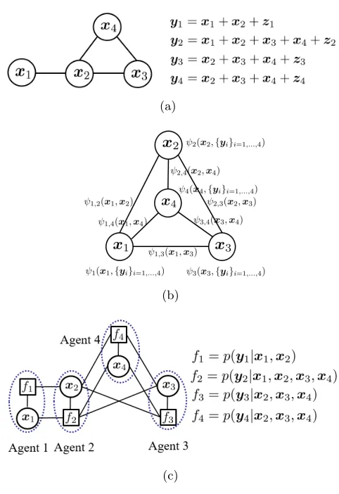
First, messages are passed between pairs of agents in EMRF, which according to the definition (5) includes not only those direct neighbors, but also pairs that are two hops away but share a common neighbor. This is illustrated in Fig. 1, where Fig. 1(a) shows a network of 4 agents with a line between two neighboring agents indicating the availability of a physical communication link, and Fig. 1(b) shows the equivalent pairwise graph. For this example, in the physical network, there is no direct connection between agents 1 and 4, nor between agents 1 and 3. But in the pairwise representation, those connections are present. We summarize the above observations in the following remark.
Remark 1 For a network with communication edge setENet and local observations
follow-ing (1), the correspondfollow-ing MRF graph edge set satisfies EMRF ⊇ ENet. Thus, Gaussian BP for Gaussian MRFs cannot be applied to the distributed inference problem with the local observation model (1).3
The consequence of the above findings is that, not only does information need to be shared among agents two hops away from each other to construct the edge potential func-tion in (7), but also the messages (8) may be required to be exchanged among non-direct neighbors, where a physical communication link is not available. This complicates signifi-cantly the message exchange scheduling.
Secondly, even if the message scheduling between non-neighboring agents can be re-alized, the convergence of (8) is not guaranteed in loopy networks. For Gaussian MRF with scalar variables, sufficient convergence conditions have been proposed in (Weiss and Freeman, 2001a; Malioutov et al., 2006; Su and Wu, 2015). However, depending on how the factorization of the underlying joint Gaussian distribution is performed, Gaussian BP may exhibit different convergence properties as different factorizations (different Gaussian models) lead to fundamentally different recursive update structures. Furthermore, these results apply only to scalar Gaussian BP, and extension to vector-valued Gaussian BP is nontrivial as we show in this paper.
The next section derives distributed vector inference based on Gaussian BP with high order interactions (beyond pairwise connections), where information sharing and message exchange requirement conform to the physical network topology. Furthermore, convergence conditions will be studied in Section 4, and we show in Section 5 that the convergence condition obtained is strictly weaker than, i.e., subsumes the convergence conditions in (Weiss and Freeman, 2001a; Malioutov et al., 2006; Su and Wu, 2015).
(a)
(b)
(c)
Figure 1: (a) A physical network with 4 agents, where {1,2} and {2,3,4} are two groups of agents that are within the communication range of each other, respectively. xi is the local unknown vector, and yi is the local observation at agent i that
follows (1); (b) The corresponding MRF of Fig. 1 (a) withψn
xn,{yi}i∈n∪I(n)
andψn,i(xn,xi) defined in (6) and (7), respectively. (c) The corresponding factor
graph of Fig. 1 (a) withfi defined in (10). Since p(xi) does not involve message
passing, thep(xi) associated to each variable node is not drawn to keep the figure
3. Distributed Inference with Vector-Valued Gaussian BP and Non-Pairwise Interaction
The joint distribution p(x)p(y|x) is first written as the product of the prior distribution and the likelihood function of each local linear Gaussian model in (1) as
p(x)p(y|x) = Y
n∈V p(xn)
Y
n∈V p
yn| {xi}i∈n∪I(n)
| {z }
,fn
. (10)
To facilitate the derivation of the distributed inference algorithm, the factorization in (10) is expressed in terms of a factor graph (Kschischang et al., 2001), where every vector variable xiis represented by a circle (called variable node) and the probability distribution of a vector
variable or a group of vector variables is represented by a square (called factor node). A variable node is connected to a factor node if the variable is involved in that particular factor. For example, Fig. 1(c) shows the factor graph representation for the network in Fig. 1(a).
We derive the Gaussian BP algorithm over the corresponding factor graph to learn xn
for all n ∈ V (Kschischang et al., 2001). It involves two types of messages: one is the message from a variable nodexj to its neighboring factor node fn, defined as
m(`)j→fn(xj) =p(xj)
Y
fk∈B(j)\fn
m(`fk−→1)j(xj), (11)
where B(j) denotes the set of neighbouring factor nodes of xj, and m(` −1)
fk→j(xj) is the
message from fk toxj at time `−1. The second type of message is from a factor node fn
to a neighboring variable node xi, defined as
m(`)fn→i(xi) =
Z
· · ·
Z
fn×
Y
j∈B(fn)\i
m(`)j→fn(xj) d{xj}j∈B(fn)\i, (12)
where B(fn) denotes the set of neighboring variable nodes of fn. The process iterates
between equations (11) and (12). At each iteration`, the approximate marginal distribution, also referred to as belief, onxi is computed locally at xi as
b(`)BP(xi) =p(xi)
Y
fn∈B(i)
m(`)fn→i(xi). (13)
In the sequel, we derive the exact expressions for the messages m(`)j→fn(xj),m(`)fn→i(xi),
and beliefb(`)BP(xi). First, let the initial messages at each variable node and factor node be
in Gaussian function forms as
m(0)fn→i(xi)∝exp
−1
2||xi−v
(0) fn→i||
2
J(0)fn→i
. (14)
In Appendix A, it is shown that the general expression for the message from variable node j to factor node fnis
m(`)j→fn(xj)∝exp
−1
2||xj−v
(`) j→fn||
2
J(`)j→fn
with
J(`)j→fn =W−j1+ X
fk∈B(j)\fn
J(`fk−→1)j, (16)
v(`)j→fn =hJ(`)j→fni−1
X
fk∈B(j)\fn
J(`fk−→1)jv(`fk−→1)j
, (17)
where J(`fk−→1)j and v(`fk−→1)j are the message information matrix (inverse of covariance ma-trix) and mean vector received at variable node j at the (`−1)-th iteration, respectively. Furthermore, the message from factor node fn to variable nodeiis given by
m(`)fn→i(xi)∝α(`)fn→iexp
−1
2||xi−v
(`) fn→i||
2
J(`)fn→i
, (18)
with
J(`)fn→i =ATn,i
Rn+
X
j∈B(fn)\i
An,j
h
J(`)j→fn
i−1
ATn,j
−1
An,i, (19)
v(`)fn→i =hJfn(`)→ii−1ATn,i
Rn+
X
j∈B(fn)\i
An,j
h
J(`)j→fni−1ATn,j
−1 yn−
X
j∈B(fn)\i
An,jv(`)j→fn
,
(20)
and
α(`)fn→i ∝
Z
. . .
Z
exp
−1
2z
TΛ(`) fn→iz
dz. (21)
In (21),Λ(`)fn→iis a diagonal matrix containing the eigenvalues ofATn,{B(fn)\i}R−n1An,{B(fn)\i}+
J(`){B(fn)\i}→fn, withAn,{B(fn)\i}denoting a row block matrix containingAn,j as row elements
for allj∈ B(fn)\iarranged in ascending order, andJ(`){B(fn)\i}→fn denoting a block diagonal
matrix withJ(`)j→fn as its block diagonal elements for allj∈ B(fn)\iarranged in ascending
order.
Obviously, the validity of (18) depends on the existence of α(`)fn→i. It is evident that (21) is the integral of a Gaussian distribution and equals to a constant when Λ(`)fn→i 0 or equivalently ATn,{B(fn)\i}R−n1An,{B(fn)\i}+J(`){B(fn)\i}→fn 0.Otherwise,α(`)fn→i does not
exist. Therefore, the necessary and sufficient condition for the existence ofm(`)fn→i(xi) is
An,T{B(fn)\i}Rn−1An,{B(fn)\i}+J (`)
{B(fn)\i}→fn 0. (22)
In general, the necessary and sufficient condition is difficult to be verified, asJ(`){B(fn)\i}→fn changes in each iteration. However, as R−n1 0, it can be decomposed asR−n1 =Re
T nRen.
Then
An,T{B(fn)\i}Rn−1An,{B(fn)\i} =
e
RnAn,{B(fn)\i}
T
e
RnAn,{B(fn)\i}
Hence, one simple sufficient condition to guarantee (22) isJ(`){B(fn)\i}→fn 0or equivalently its diagonal block matrix J(`)j→fn 0 for all j∈ B(fn)\i. The following lemma shows that
setting the initial message covariancesJ(0)fn→i 0 for all (n, i)∈ ENet guaranteesJ(`)j→fn 0 for`≥1 and all (n, j)∈ ENet.
Lemma 2 Let the initial messages at factor node fk be in Gaussian forms with the initial
message information matrix J(0)f
k→j 0 for all k ∈ V and j ∈ B(fk). Then J (`)
j→fn 0
and J(`)fk→j 0 for all ` ≥1 with j ∈ V and fn, fk ∈ B(j). Furthermore, in this case, all
messages m(`)j→fn(xj) andm(`)fk→j(xi) are well defined.
Proof See Appendix B.
For this factor graph based approach, according to the message updating procedure (15) and (18), message exchange is only needed between neighboring agents (an agent refers to a variable-factor pair as shown in Fig. 1 (c)). For example, the messages transmitted from agentn to its neighboring agent iare m(`)fn→i(xi) andm(`)n→fi(xn). Thus, the factor graph
does impose a clear messaging schedule, and the message passing scheme given in (11) and (12) conforms with the network topology. Furthermore, if the messages m(`)j→fn(xj)
and m(`)fn→i(xi) exist for all ` (which can be achieved using Lemma 2), the messages are
Gaussian, therefore only the corresponding mean vectors and information matrices (inverse of covariance matrices) are needed to be exchanged.
Finally, if the Gaussian BP messages exist, according to the definition of belief in (13), b(`)BP(xi) at iteration `is computed as
b(`)BP(xi) =p(xi)
Y
fn∈B(i)
m(`)fn→i(xi),
∝ Nxi|µ(`)i ,P(`)i
,
where the belief covariance matrix
P(`)i =
W
−1 i +
X
fn∈B(i)
J(`)fn→i
−1
, (23)
and mean vector
µ(`)i =P(`)i
X
fn∈B(i)
J(`)fn→iv(`)fn→i
. (24)
Remark 3 We assume that Rn 0 in this paper. If, however, some of the
observa-tions are noiseless, for example, Rn = 0, the local observation is yn =
P
i∈n∪I(n)An,ixi.
Then the corresponding local likelihood function is represented by the Dirac measure δ(yn−
P
i∈n∪I(n)An,ixi). Suppose, for example, there is only one agent with Rn = 0, and all
others are Ri 0. The the joint distribution is written as
p(x)p(y|x) =δ(yn− X i∈n∪I(n)
An,ixi)
Y
j∈V p(xj)
Y
k∈V p
yk| {xi}i∈k∪I(k)
.
In this case, ifAn,n is invertible, then, by the definition of the Dirac measure, we havexn=
A−n,n1
yn−P
i∈I(n)An,ixi
. By substituting this equation into all of the likelihood functions involving xn, we have the equivalent joint distribution as in (10) with all the likelihood
functions having a positive definite noise covariance. We thereafter can apply Gaussian BP to this new factorization and the convergence analysis in this paper still applies. Therefore, without loss of generality, we assume all Rn 0. Note that when Rn = 0 for all n, this
problem is equivalent to solving algebraic equations, which has been studied in (Shental et al., 2008b) using Gaussian BP.
4. Convergence Analysis
The challenge of deploying the Gaussian BP algorithm for large-scale networks is in de-termining whether it will converge or not. In particular, it is generally known that if the factor graph contains cycles, the Gaussian BP algorithm may diverge. Thus, determining convergence conditions for the Gaussian BP algorithm is very important. Sufficient condi-tions for the convergence of Gaussian BP with scalar variables in loopy graphs are available in (Weiss and Freeman, 2001a; Malioutov et al., 2006; Su and Wu, 2015). However, these conditions are derived based on pairwise graphs with local functions in the form of (6) and (7). This contrasts with the model considered in this paper, where the fn in (10) involves
high-order interactions between vector variables, and thus the convergence results in (Weiss and Freeman, 2001a; Malioutov et al., 2006; Su and Wu, 2015) cannot be applied to the factor graph based vector-form Gaussian BP.
Due to the recursive updating property of m(`)j→fn(xj) andm(`)fn→i(xi) in (15) and (18),
the message evolution can be simplified by combining these two kinds of messages into one. By substituting J(`)j→fn in (16) into (19), the updating of the message covariance matrix inverse, referred to as message information matrix in the following, can be denoted as
J(`)fn→i = ATn,i
Rn+
X
j∈B(fn)\i
An,j
W−j1+ X
fk∈B(j)\fn
J(`fk−→1)j
−1
ATn,j
−1
An,i
, Fn→i
n
J(`fk−→1)jo
(fk,j)∈Be(fn,i)
, (25)
where Be(fn, i) = {(fk, j)|j ∈ B(fn)\i, fk∈ B(j)\fn}. Observing that J
(`)
fn→i in (25) is
characteri-zation ofJ(`)fn→i and v(`)fn→i, we will further investigate the convergence of belief covariances and means in (23) and (24), respectively.
Note that computing P(`)j requires all the incoming messages from neighboring nodes including J(`)fn→j as shown in (23) by replacing the subscript i with j in (23). However, according to (25), when computing J(`)fn→i the quantityJ(`fn−→1)j is excluded, i.e., the quantity inside the inner square brackets equals [P(`j−1)]−1−J(`−1)
fn→j. Therefore, one cannot compute
J(`)fn→i fromP(`)j alone.
4.1 Convergence of Message Information Matrices
To efficiently represent the updates of all message information matrices, we introduce the following definitions. Let
J(`−1) ,Bdiag
n
J(`fn−→1)io
n∈V,i∈B(fn)
be a block diagonal matrix with diagonal blocks being the message information matrices in the network at time `−1 with index arranged in ascending order first on n and then on i. Using the definition of J(`−1), the term P
fk∈B(j)\fnJ (`−1)
fk→j in (25) can be written as
Ξn,jJ(`−1)ΞTn,j, where Ξn,j is for selecting appropriate components from J(`−1) to form the
summation. Further, define Hn,i =
h
{An,j}j∈B(fn)\i
i
, Ψn,i = Bdiag
n
W−j1
o
j∈B(fn)\i
and Kn,i = Bdiag
{Ξn,j}j∈B(fn)\i
, all with component blocks arranged with ascending order on j. Then (25) can be written as
J(`)fn→i =ATn,i
Rn+Hn,i
h
Ψn,i+Kn,i
I|B(fn)|−1⊗J(`−1)
KTn,i
i−1
HTn,i
−1
An,i. (26)
Now, we define the function F , {F1→k, . . . ,Fn→i, . . . ,Fn→M} that satisfies J(`) = FJ(`−1)
. Then, by stacking J(`)fn→i on the left side of (26) for all n and i as the block diagonal matrix J(`), we obtain
J(`) = AT
Ω+HhΨ+KIϕ⊗J(`−1)
KTi−1HT −1A,
, FJ(`−1)
, (27)
whereA,H,Ψ, andKare block diagonal matrices with block elementsAn,i,Hn,i,Ψn,i, and
Kn,i, respectively, arranged in ascending order, first onnand then oni(i.e., the same order
asJ(`)fn→i inJ(`)). Furthermore,ϕ=PM
n=1|B(fn)|(|B(fn)| −1) andΩis a block diagonal
matrix with diagonal blocksI|B(fn)|⊗Rnwith ascending order onn. We first present some
properties of the updating operatorF(·), the proofs being provided in Appendix C.
P 4.1: FJ(`)
FJ(`−1)
, ifJ(`)J(`−1)0. P 4.2: αFJ(`)
FαJ(`)
and Fα−1J(`)
α−1FJ(`)
, ifJ(`)0 and α >1. P 4.3: DefineU ,ATΩ−1A and L,AT
Ω+HΨ−1HT−1
A. With arbitraryJ(0) 0,
FJ(`)
is bounded byU FJ(`)
L0 for`≥1.
Based on the above properties of F(·), we can establish the convergence of the infor-mation matrices.
Theorem 5 There exists a unique positive definite fixed pointJ∗ for the mapping F(·).
Proof The set [L,U] is a compact set. Further, according to Proposition 4, P 4.3, for arbitrary J(0) 0, F maps [L,U] into itself starting from ` ≥ 1. Next, we show that [L,U] is a convex set. Suppose that X, Y ∈ [L,U], and 0 ≤ t ≤ 1, then tX−tL and (1−t)Y−(1−t)L are positive semidefinite (p.s.d.) matrices. Since the sum of two p.s.d. matrices is a p.s.d. matrix, tX+ (1−t)Y L. Likewise, it can be shown that tX+ (1−t)Y U. Thus, the continuous function F maps a compact convex subset of the Banach space of positive definite matrices into itself. Therefore, the mapping F has a fixed point in [L,U] according to Brouwer’s Fixed-Point Theorem (Zeidler, 1985), and the fixed point is positive definite (p.d.).
Next, we prove the uniqueness of the fixed point. Suppose that there exist two fixed pointsJ∗ 0 andeJ
∗
0. SinceJ∗ andJe
∗
are p.d., their componentsJ∗fn→i andeJ
∗
fn→i are
also p.d. matrices. For the component blocks of J∗ and Je
∗
, there are two possibilities: 1)
e
J∗fn→i−J∗fn→i 0orJe
∗
fn→i−J ∗
fn→iis indefinite for somen, i∈ V, and 2)eJ
∗
fn→i−J ∗
fn→i 0
for all n, i∈ V.
For the first case, there must exist ξfn,i > 1 such that ξfn,iJ∗fn→i −eJ
∗
fn→i has one or
more zero eigenvalues, while all other eigenvalues are positive. Pick the component matrix with the maximum ξfn,i among those falling into this case, sayξf%,τ, then, we can write
ξf%,τJ∗f%→τ−eJ
∗
f%→τ 0, (28)
or in terms of the information matrices for the whole network
ξf%,τJ∗ Je
∗
0, ξf%,τ >1. (29)
Applying F on both sides of (29), according to the monotonic property of F(·) as shown in Proposition 4, P 4.1, we have
F ξf%,τJ∗
FJe
∗
=eJ
∗
, (30)
where the equality is due to Je
∗
being a fixed point. According to Proposition 4, P 4.2, ξf%,τF(J∗) F ξf%,τJ∗
. Therefore, from (30), we obtain ξf%,τJ∗eJ
∗
. Consequently,
ξf%,τJ∗f%,τ eJ
∗ f%,τ.
But this contradicts withξf%,τJ∗f%,τ−Je
∗
f%,τ having one or more zero eigenvalues as discussed
before (28). Therefore, we must haveJ∗ =eJ
On the other hand, if we have case two, which isJe
∗
fn→i−J∗fn→i0 for alln, i∈ V, we
can repeat the above derivation with the roles of Je
∗
and J∗ reversed, and we would again obtain J∗=eJ
∗
. Consequently, J∗ is unique.
Lemma 2 states that with arbitrary p.s.d. initial message information matrices, the message information matrices will be kept as p.d. at every iteration. On the other hand, Theorem 5 indicates that there exists a unique fixed point for the mapping F. Next, we will show that, with arbitrary initial value J(0) 0,J(`) converges to a unique p.d. matrix.
Theorem 6 The matrix sequence n
J(`)
o
l=0,1,... defined by (27) converges to a unique
pos-itive definite matrix J∗ for any initial covariance matrix J(0)0.
Proof With arbitrary initial value J(0) 0, following Proposition 4, P 4.3, we have U J(1) L 0. On the other hand, according to Theorem 5, (27) has a unique fixed point J∗ 0. Notice that we can always choose a scalarα >1 such that
αJ∗ J(1) L. (31)
Applying F(·) to (31)` times, and using Proposition 4, P 4.1, we have
F`(αJ∗) F`+1J(0)
F`(L), (32)
whereF`(X) denotes applying F onX `times.
We start from the left inequality in (32). According to Proposition 4, P 4.2, αJ∗ F(αJ∗). Applying F again gives F(αJ∗) F2(αJ∗). Applying F(·) repeatedly, we can obtain F2(αJ∗
) F3(αJ∗
) F4(αJ∗
), etc. Thus F`(αJ∗
) is a non-increasing sequence with respect to the partial order induced by the cone of p.s.d. matrices as`increases. Fur-thermore, sinceF(·) is bounded below byL,F`(αJ∗) converges. Finally, since there exists only one fixed point forF(·), liml→∞F`(αJ∗) =J∗. On the other hand, for the right hand side of (32), as F(·) L, we have F(L) L. Applying F repeatedly gives successively
F2(L) F(L), F3(L) F2(L), etc. So, F`(L) is an non-decreasing sequence (with
respect to the partial order induced by the cone of p.s.d. matrices). Since F(·) is upper bounded by U,F`(L) is a convergent sequence. Again, due to the uniqueness of the fixed
point, we have liml→∞F`(L) =J∗. Finally, taking the limit with respect to `on (32), we have liml→∞F`
J(0)
=J∗,for arbitrary initialJ(0)0.
Remark 7 According to Theorem 6, the information matrix J(`)fn→i converges if all initial information matrices are p.s.d., i.e., J(0)fn→i 0 for all i ∈ V and fn ∈ B(i). However,
for the pairwise model, the messages are derived based on the classical Gaussian MRF based factorization (in the form of equations (6) and (7)) of the joint distribution. This differs from the model considered in this paper, where the factor fn follows equation (10),
Gaussian MRF based factorization, the information matrix does not necessarily converge for all initial nonnegative values (for the scalar variable case) as shown in (Malioutov et al., 2006; Moallemi and Roy, 2009a).
Remark 8 Due to the computation of J(`)fn→i being independent of the local observations
yn, as long as the network topology does not change, the converged value J∗fn→i can be
precomputed offline and stored at each agent, and there is no need to re-compute J∗fn→i
even if yn varies.
Another fundamental question is how fast the convergence is, and this is the focus of the discussion below. Since the convergence of a dynamic system is often studied with respect to the part metric (Chueshov, 2002), in the following, we start by introducing the part metric.
Definition 9 Part (Birkhoff ) Metric (Chueshov, 2002): For arbitrary symmetric matrices
X and Y with the same dimension, if there exists α ≥ 1 such that αX Y α−1X, X
and Y are called the parts, and d (X,Y) ,inflogα:αXYα−1X, α≥1 defines a metric called the part metric.
As it is useful to have an estimate of the convergence rate of J(`) in terms of the more standard induced matrix norms, we further introduce the notion of monotone norms. The norms|| · ||2 and || · ||F (Frobenus norm) are monotone norms.
Definition 10 Monotone Norm (Ciarlet, 1989, 2.2-10): A matrix norm k · k is monotone if
X0,YX⇒ kYk ≥ kXk.
Next, for arbitrary >0, we will show thatnJ(`)o
l=1,..approaches the -neighborhood
of the fixed point J? exponentially fast with respect to the monotone norm. To this end, for a fixed >0, define the set
C=
n
J(`)|UJ(`)J∗+I
o
∪nJ(`)|J∗−IJ(`)L
o
. (33)
Theorem 11 With the initial message information matrix set to be an arbitrary p.s.d. matrix, i.e., J(0)fn→i 0, the sequence
n
J(`)
o
l=0,1,... approaches an arbitrarily small
neigh-borhood of the fixed positive definite matrix J∗ at an exponential rate with respect to any matrix norm.
Proof Fix >0 and consider the setCdefined in (33). It suffices to show that the quantity
kJ(`)−J∗k, wherek · kis a monotone norm as defined in Definition 10, decays exponentially as long asJ(s)∈ C for alls∈ {0,1,· · ·`}. To this end, forJ(`)∈ C, andJ∗ 6∈ C (necessarily), according to Definition 9, we have dJ(`),J∗,infnlogα:αJ(`)J∗ α−1J(`)o. Since d
J(`),J∗
is the smallest number satisfying αJ(`)J∗ α−1J(`), this is equivalent to exp
n
d
J(`),J∗
o
J(`) J∗exp
n
−d
J(`),J∗
o
Applying Proposition 4, P 4.1 to (34), we have
FexpndJ(`),J∗oJ(`) F(J∗) Fexpn−dJ(`),J∗oJ(`). Then applying Proposition 4, P 4.2 and considering that exp
n
d
J(`),J∗
o
> 1 and
exp
n
−d
J(`),J∗
o
<1, we obtain
expndJ(`),J∗oFJ(`) F(J∗)expn−dJ(`),J∗oFJ(`).
Notice that, for arbitrary p.d. matrices X and Y, if X−kY 0, then, by definition, we have xTXx−kxTYx >0 for arbitraryx6=0. Then, there must exist o >0 that is small enough such thatxTXx−(k+o)xTYx>0 or equivalentlyX(k+o)Y. Thus, as exp (·) is a continuous function, there must exist some 4d>0 such that
expn−4d + dJ(`),J∗oFJ(`) F(J∗)expn4d−dJ(`),J∗oFJ(`). (35) Now, using the definition of the part metric, (35) is equivalent to
−4d + d
J(`),J∗
≥d
FJ(`)
,F(J∗)
.
Hence, we obtain dFJ(`),F(J∗)<dJ(`),J∗. Since this result holds for anyJ(`)∈ C, we also have d
FJ(`)
,F(J∗)
< cd
J(`),J∗
, wherec= supJ(`)∈C
d(F(J(`)),F(J∗))
d(J(`),J∗) < 1. Since J(`+1)=FJ(`)and J∗=F(J∗), we have
d
J(`),J∗
< c`d
J(0),J∗
. (36)
According to (Krause and Nussbaum, 1993, Lemma 2.3), the convergence rate of||J(`)−
J∗||can be determined by that of dJ(`),J∗. More specifically,
||J(`)−J∗|| ≤2 exp
n
d
J(`),J∗
o
−exp
n
−d
J(`),J∗
o
−1
min
n
||J(`)||,||J∗||o, (37) where|| · || is a monotone norm defined on the p.s.d. cone:
As we show in Proposition 4, P 4.3 thatJ(`) is bounded, then||J(`)||and ||J∗||must be finite. Letζ be the largest value of minn||J(`)||,||J∗||ofor all{J(`)}with`≥0, thenζ >0. According to (36) and (37), we have that
||J(`)−J∗||< ζ
2 exp
n
c`d0
o
−exp
n
−c`d0
o
−1
, (38)
with 0 < c < 1 and d0 = d
J(0),J∗, which is a constant. The above inequality is equivalent to
||J(`)−J∗||< ζ
3 exp
n
c`d0
o
−exp
n
c`d0
o
−exp
n
−c`d0
o
−1
Since both exp
c`d0 and exp
−c`d0 are positive and exp
c`d0 exp
−c`d0 = 1,
ac-cording to the arithmetic-geometric mean inequality, we have expc`d0 + exp
−c`d0 ≥
2 exp
c`d 0 exp
−c`d 0
1/2
= 2. Then, the right-hand side of (39) is further amplified, and we obtain
||J(`)−J∗||< ζ3 expnc`d0
o
−3= 3ζexpnc`d0
o
−1.
Therefore, the sequence nJ(`)o
l=0,1,... approaches the -neighborhood (and hence any
arbi-trarily small neighborhood) of the fixed positive definite matrix J∗ at an exponential rate with respect to any matrix norm.
The physical meaning of Theorem 11 is that the distance betweenJ(`) andJ∗ decreases ex-ponentially fast before J(`) enters J∗’s neighborhood, which can be chosen to be arbitrarily small. Next, we study how to choose the initial value J(0) so thatJ(`) converges faster. Theorem 12 With 0J(0) L, J(`) is a monotonic increasing sequence, and J(`) con-verges most rapidly with J(0)=L. Moreover, withJ(0)U,J(`) is a monotonic decreasing sequence, and J(`) converges most rapidly with J(0) =U.
Proof Following Proposition 4, P 4.3, it can be verified that for 0 J(0) L, we have J(1) J(0). Then, according to Proposition 4, P 4.1, and by induction, this relationship can be extended to J(`) . . .J(1) J(0), which states that J(`) is a monotonic increasing sequence. Now, suppose that there are two sequences J(`) and eJ
(`)
that are started with
different initial values 0 J(0) ≺ L and 0 eJ
(0)
≺ L, respectively. Then these two sequences are monotonically increasing and bounded byJ∗. To prove thatJ(0)=Lleads to the fastest convergence, it is sufficient to prove that J(`) Je
(`)
for`= 0,1. . .. First, note
that J(0) eJ
(0)
. Assume J(n) eJ
(n)
for some n ≥0. According to Proposition 4, P 4.1,
we haveFJ(n) FJe
(n)
, or equivalentlyJ(n+1) eJ
(n+1)
. Therefore, by induction, we
have proven that, with J(0) = L, J(`) converges more rapidly than with any other initial value0J(0) ≺L.
With similar logic, we can show that, with J(0) U, J(`) is a monotonic decreasing sequence; and, withJ(0) =U,J(`) converges more rapidly than that with any other initial valueJ(0) U.
Notice that it is a common practice in the Gaussian BP literature that the initial infor-mation matrix (or inverse variance for the scalar case) is set to be0, i.e., J(0)fn→i =0(Weiss and Freeman, 2001a; Malioutov et al., 2006). Theorem 12 reveals that there is a better choice to guarantee faster convergence.
4.2 Convergence of Message Mean Vector
According to Theorems 6 and 11, as long as we choose J(0)fk→j 0 for all j ∈ V and fk∈ B(j), the distance betweenJ(`)fk→j andJ
∗
fk→j decreases exponentially fast beforeJ (`) fk→j
enters J∗f
according to (16),
h
J(`)j→fn
i−1
also converges to a p.d. matrix onceJ(`)fk→j converges, and the converged value for
h
J(`)j→fn
i−1
is denoted by J∗j→fn
−1
. Then for arbitrary initial value
v(0)fk→j, the evolution of v(`)j→fn in (17) can be written in terms of the converged message information matrices, which is
v(`)j→fn =J∗j→fn
−1 X
fk∈B(j)\fn
J∗fk→jv (`−1)
fk→j. (40)
Using (20), and replacing indices j,i,nwith z,j,krespectively,v(`fk−→1)j is given by
v(`fk−→1)j = [J∗fk→j]−1ATk,j
"
Rk+
X
z∈B(fk)\j
Ak,z
J∗z→fk−1
ATk,z
| {z }
,Mk,j
#−1 yk−
X
z∈B(fk)\j
Ak,zv(` −1) z→fk
.
(41)
Putting (41) into (40), we have
v(`)j→fn =bj→fn−
X
fk∈B(j)\fn
X
z∈B(fk)\j
[J∗j→fn]−1ATk,jM−k,j1Ak,zv(` −1)
z→fk, (42)
where bj→fn = [J∗j→fn]−1
P
fk∈B(j)\fnA T k,jM
−1
k,jyk. The above equation can be further
written in compact form as
v(`)j→fn =bj→fn−Qj→fnv(` −1),
with the column vector v(`−1) containing vz(`→−1)fk for all z ∈ V and fk ∈ B(z) as subvector
with ascending index first on z and then on k. The matrix Qj→fn is a row block matrix
with component block [J∗j→fn]−1ATk,jM−k,j1Ak,z if fk ∈ B(j)\fn and z∈ B(fk)\j, and 0
otherwise. LetQbe the block matrix that stacksQj→fn with the order first onj and then on n, and b be the vector containing bj→fn with the same stacking order as Qj→fn. We
have
v(`)=−Qv(`−1)+b, `≥1,2, . . . . (43) It is known that for arbitrary initial value v(0), v(`) converges if and only if the spectral
radiusρ(Q)<1 (Demmel, 1997, pp. 280). Since the elements of v(0), i.e., v(0)j→fn, depends onv(0)fk→j, we can choose arbitraryv(0)fk→j. Furthermore, asv(`)depends on the convergence
of J(`), we have the following result.
Theorem 13 The vector sequencev(`) l=1,2,... defined by (43) converges to a unique value under any initial value
n
v(0)fk→j
o
k∈V,j∈B(fk)and initial message information matrix J (0)0
The row block matrix Qj, a row block ofQ, contains only block entries0 and Qj→fn. When the observation model (1) reduces to the pairwise model, where only two unknown variables are involved in each local observation, it can be shown that Qj and Qi are or-thogonal ifi6=j. A distributed convergence condition is obtained utilizing this orthogonal property in Du et al. (2017a). However, for the more general case studied in this paper, properties of Qj and Qneed to be further exploited to show whenρ(Q)<1 is satisfied.
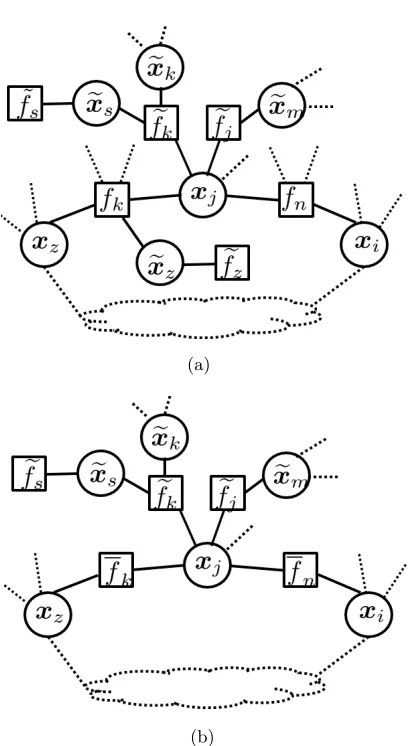
In the sequel, we will show that ρ(Q)<1 is satisfied for a single loop factor graph with multiple chains/trees (an example is shown in Fig. 2), thus Gaussian BP converges in such a topology. Although Weiss (2000) shows the convergence of Gaussian BP on the MRF with a single loop, the analysis cannot be applied here since the local observations model (1) is different from the pairwise model in (Weiss, 2000).
Theorem 14 For any factor graph that is the union of a single loop and a forest, with arbitrary positive semi-definite initial information matrix, i.e., J(0)fn→i 0for all i∈ V and
fn ∈ B(i), the message information matrix J (`)
fn→i and mean vector v (`)
i→fn is guaranteed to
converge to their corresponding unique points.
Proof In this proof, Fig. 2 is being used as a reference throughout. For a single loop factor graph with chains/trees as shown in Fig. 2 (a), there are two kinds of nodes. One is the factors/variables in the loop, and they are denoted by fn/xj. The other is the
factors/variables on the chains/trees but outside the loop, denoted asfek/ezi. Then message
from a variable node to a neighboring factor node on the graph can be categorized into three groups:
1) message on a tree/chain passing towards the loop, e.g., m∗ e
z→fk(exz) and m
∗
e s→fke
(xes) ;
2) message on a tree/chain passing away from the loop, e.g., m(`) j→fek
(xj), m(`) e s→fse
(xs) and m(`)
e z→fze
(xz);
3) message in the loop, e.g.,m(`)j→fn(xj), m(`)z→fk(xz) and m (`)
i→fn(xi).
According to (11), computation of the messages in the first group does not depend on messages in the loop and is thus convergence guaranteed. Therefore, the message iteration number is replaced with a ∗ to denote the converged message. Also, from the definition of message computation in (11), if messages in the third group converge, the second group messages should also converge. Therefore, we next focus on showing the convergence of messages in the third group.
For a factor nodefkin the loop withxz andxj being its two neighboring variable nodes
in the loop and xez being its neighboring variable node outside the loop, according to the
definition of message computation in (12), we have
m(`)fk→j(xj) =
Z Z
fk×m (`) z→fk(xz)
Y
e z∈B(fk)\j
m∗ e
z→fk(exz) d{exz}
e
z∈B(fk)\j dxz,
=
Z
m(`)z→fk(xz)
Z
fk×
Y
e z∈B(fk)\j
m∗ e
z→fk(exz) d{exz}ez∈B(fk)\j
dxz.
(a)
(b)
As shown in Lemma 2,m∗ e
z→fk(exz) must be in Gaussian function form, which is denoted by
m∗ e
z→fk(xez)∝ N
e
xz|v∗ e z→fk,
h
J∗
e z→fk
i−1
. Besides, from (1) we obtain
fk=N
yk|Ak,zxz+Ak,jxj+ X
e z∈B(fk)
Ak,ezxez,Rk
.
It can be shown that the inner integration in the second line of (44) is given by
N yk|Ak,zxz+Ak,jxj,Rk
,fk,
where the overbar is used to denote the new constant matrix or vector. Then (44) can be written as
m(`)fk→j(xj) =
Z
fk×m(`)z→fk(xz) dxz. (45)
Comparing (45) with (12), we obtainm(`)f
k→j(xj) as ifm (`) fk→j
(xj) is being passed to a factor
nodefk. Therefore, a factor graph with a single loop and multiple trees/chains is equivalent to a single loop factor graph in which each factor node has no neighboring variable node outside the loop. As a result, the example of Fig. 2 (a) is equivalent to Fig. 2 (b). In the following, we focus on this equivalent topology for the convergence analysis.
Note that, for arbitrary variable node j in the loop, there are two neighboring factor nodes in the loop. Further, using the notation for the equivalent topology, (42) is reduced to
v(`)
j→fn
=−hJ∗j→f
n
i−1
ATk,jT−k,j1Ak,zv(` −1) z→fk
+bj→f
n−
X
e
fk∈B(j)\fn
X
e
s∈B(fke)\j
h
J∗j→f
n
i−1
ATk,jM−k,j1Ak,esv∗ e s→fke
| {z }
,cj→f n
, (46)
wherev∗
e s→fek
is the converged mean vector on the chain/tree;
bj→f
n =
h
J∗j→f
n
i−1 X
fk∈B(j)\fn
ATk,jM−k,j1yk
withMk,j =Rk+P e
s∈B(fek)\jAk,es
h
J∗
e s→fke
i−1
ATk,
e s, and
Tk,j =Rk+Ak,z
h
J∗z→f
k
i−1
ATk,z, (47)
with xz and fk in the loop where fk ∈ B(j)\fn and xz ∈ B fk
\j. By multiplying
h
J∗j→f
n
i1/2
on both sides of (46), and definingβ(`) j→fn
=hJ∗j→f
n
i1/2
v(`)
j→fn
, we have
β(`) j→fn
=−hJ∗j→f
n
i−1/2
ATk,jT−k,j1Ak,z
h
J∗z→f
k
i−1/2
β(`−1) z→fk
+hJ∗j→f
n
i1/2
cj→f
Letβ(`−1) containβ(`−1) z→fk
for allxz withz∈ B fk
andfkbeing in the loop, and the index is arranged first onkand then onz. Then, the above equation is written in a compact form as
β(`) j→fn
=−Qj→f
nβ
(`−1)+hJ∗ j→fn
i1/2
cj→f
n, (49)
whereQj→f
n is a row block matrix with the only nonzero block
h
J∗j→f
n
i−1/2
ATk,jT−k,j1Ak,z
h
J∗z→f
k
i−1/2
located at the position corresponding to the positionβ(`) z→fk
inβ(`). Then letQbe a matrix that stacks Qj→f
n as its row, wherej and fn are in the loop withj ∈ B fn
. Besides, let
c be the vector containing the subvector
h
J∗j→f
n
i1/2
cj→f
n with the same order as Qj→fn
inQ. We have
β(`) =−Qβ(`−1)+c. (50) SinceQis a square matrix,ρ(Q)≤qρ QQT
and thereforeρ QQT
<1 is the sufficient
condition for the convergence ofβ(`). We next investigate the elements in QQT. Due to the single loop structure of the graph, every β(`)
j→fn
in (48) would be dependent
on a unique β(`) z→fk
, where fk ∈ B(j)\fn and z ∈ B fk\j (i.e., the message two hops backward along the loop in the factor graph). Thus, the position of the non-zero block in Qj→f
n will be different and non-overlapping for different combinations of (j, fn). As
a result, there exists a column permutation matrix Ξ such that QΞ is a block diagonal matrix. Therefore, (QΞ) (QΞ)T =QQT is also a diagonal matrix, and we can write
QQT =Bdiag
n
Qj→f
nQ T j→fn
o
j∈ Bfn.
As a consequence, ρ QQT<1 is equivalent to ρ
Qj→f
nQ T j→fn
<1 for all j and fn in the loop withj ∈ B fn
. Following the definition of Qj→f
n below (49), we obtain
Qj→f
nQ T j→fn =
h
J∗j→f
n
i−1/2
ATk,jT−k,j1Ak,z
h
J∗z→f
k
i−1
ATk,zT−k,j1Ak,j
h
J∗j→f
n
i−1/2
=hJ∗j→f
n
i−1/2
ATk,jT−k,j1 Tk,j−Rk
T−k,j1Ak,j
h
J∗j→f
n
i−1/2
,
(51)
where the second equation follows from the definition ofTk,jin (47). Besides, sinceRk0,
we have Tk,j−Rk ≺ Tk,j. Following P B.2 in Appendix B, and due to Tk,j = TTk,j, we
have
T−k,j1/2 Tk,j−Rk
T−k,j1/2 ≺I. (52)
Applying P B.2 in Appendix B again to (52), and making use of (51), we obtain
Qj→f
nQ T j→fn ≺
h
J∗j→f
n
i−1/2
ATk,jT−k,j1Ak,j
h
J∗j→f
n
i−1/2
According to (47), we have
ATk,jT−k,j1Ak,j =A T k,j
Rk+Ak,z
h
J∗z→f
k
i−1
ATk,z
−1
Ak,j. (54)
On the other hand, using (19), due toB fk\j=xz in the considered topology, the right
hand side of (54) isJ∗f
k→j. Therefore, (53) is further written as
Qj→f
nQ T j→fn
≺hJ∗j→f
n
i−1/2
J∗f
k→j
h
J∗j→f
n
i−1/2
. (55)
From (16), J∗j→f
n =W −1 j +J
∗ fk→j +
P
e
fk∈B(j)\fnJ ∗
e
fk→j, thus J ∗ fk→j
J∗j→f
n. Therefore,
h
J∗j→f
n
i−1/2
J∗f
k→j
h
J∗j→f
n
i−1/2
I, and, together with (55), we have
Qj→f
nQ T j→fn
≺I.
Hence ρ
Qj→f
nQ T j→fn
<1 for all j and fn in the loop andj ∈ B fn, and equivalently ρ(Q)<1. This completes the proof.
4.3 Convergence of Belief Covariance and Mean Vector
As the computation of the belief covarianceP(`)i depends on the message information matrix J(`)fn→i, using Theorems 6 and 11, we can derive the convergence and uniqueness properties of P(`)i .
Before we present the main result, we first present some properties of the part metric d (X,Y), with positive definite arguments X, Y, and 4X. The proofs are provided in Appendix D.
Proposition 15 The part metric d (X,Y) satisfies the following properties
P 15.1: d (X1+X2,Y1+Y2)≤d (X1,Y1) + d (X2,Y2);
P 15.2: d (X,Y) = d X−1,Y−1
.
We now have the following result.
Corollary 16 With arbitrary initial message information matrix J(0)fn→i 0 for all i∈ V
and fn ∈ B(i), the belief covariance matrix P(`)i converges to a unique p.d. matrix at an
exponential rate with respect to any matrix norm beforeP(`)i entersP∗i’s neighborhood, which can be chosen to be arbitrarily small.
and part metric in Definition 9, we have
d
[P(`)i ]−1,[P∗i]−1
= d
W
−1 i +
X
fn∈B(i)
J(`)fn→i,W−i 1+ X
fn∈B(i)
J∗fn→i
.
By applying P 15.1 to the above equation, we obtain
d[P(`)i ]−1,[P∗i]−1≤d W−i 1,W−i 1
+ X
fn∈B(i)
dJ(`)fn→i,J∗fn→i= X
fn∈B(i)
dJ(`)fn→i,J∗fn→i.
According to (36), for all i∈ V and fn∈ B(i), there exist ac <1 such that
dJ(`)fn→i,J∗fn→i< c`dJ(0)fn→i,J∗fn→i.
Applying the above inequality to compute hP(`)i i
−1
in (24), we obtain
d[P(`)i ]−1,[P∗i]−1< c` X fn∈B(i)
dJ(0)fn→i,J∗fn→i.
Following P 15.2, the above inequality is equivalent to
d
P(`)i ,P∗i
< c` X fn∈B(i)
d
J(0)fn→i,J∗fn→i
,
whereP
fn∈B(i)d
J(0)fn→i,J∗fn→i
is a constant. Following the same procedure as that from
(36) to (38), we can prove that P(`)i converges at an exponential rate with respect to the monotone norm beforeP(`)i entersP∗i’s neighborhood, which can be chosen to be arbitrarily small.
On the other hand, as shown in (24), the computation of the belief mean µ(`)i depends on the belief covarianceP(`)i and the message meanv(`)fn→i. Thus, under the same condition as in Theorem 13, µ(`)i is convergence guaranteed. Moreover, it is shown in (Weiss and Freeman, 2001b, Appendix) that, for Gaussian BP over a factor graph, the converged value of belief mean equals the optimal estimate in (3). Together with the convergence guaranteed topology revealed in Theorem 14, we have the following Corollary.
Corollary 17 With arbitrary J(0)fn→i 0and arbitrary v(0)fn→i for all i∈ V and fn ∈ B(i),
the mean vector µ(`)i in (24) converges to the optimal estimate bxi in (3) if and only if
ρ(Q) < 1, where Q is defined in (43). Furthermore, a sufficient condition to guarantee
5. Relationships with Existing Convergence Conditions
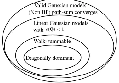
In this section, we show the relationship between our convergence condition for Gaussian BP and the recent proposed path-sum method (Giscard et al., 2016). We also show that our convergence condition is more general than the walk-summable condition (Malioutov et al., 2006) for the scalar case.
5.1 Relationship with the Path-sum Method
The path-sum method is proposed in (Giscard et al., 2012, 2013, 2016) to compute W−1+ATR−1A−1 in (3), in which the matrix inverse W−1+ATR−1A−1 is interpreted as the sum of simple
paths and simple cycles on a weighted graph. The resulting formulation is guaranteed to converge to the correct value for any valid multivariate Gaussian distribution.
The BP message update equations (16), (17), (19), and (20) can be seen as a cut-off of path-sum by retaining only self-loops and backtracks (simple cycles of lengths one and two). In the presence of a graph with one or more loops, equations (16), (17), (19), and (20) do not include the terms related to simple cycles with length larger than 2. This may be a potential cause for the possible divergence of the Gaussian BP algorithm. From this perspective, the divergence can be averted if none of the walks going around the loop(s) have weight greater than one, or equivalently, that the spectral radius of the block matrix representing the loop(s) is strictly less than one. This is an intuitive explanation of the conditionρ(Q)<1 obtained in Theorem 13. It also immediately follows from these considerations that the convergence rate is at least geometric, with a cut-off of order`yielding anO(ρ(Q)`) error4. While the path-sum framework provides an insightful interpretation of the results ob-tained in this paper, the path-sum algorithm may not be efficiently implementable in dis-tributed and parallel settings, as it requires the summation over all the paths of any length. In contrast, Gaussian BP, while paying the price of non-convergence in general loopy mod-els, makes it possible to realize parallel and fully distributed inference. In summary, though the path-sum method converges for arbitrary valid Gaussian models, it is difficult to be adapted to a distributed and parallel inference setup as the Gaussian BP method.
5.2 Relationship with the Walk-Summable Condition
We show next that, in the setup of linear Gaussian models, the condition ρ(Q) < 1 as in Corollary 17 encompasses the Gaussian MRF based walk-summable (Malioutov et al. (2006)) in terms of convergence. As all existing results on Gaussian BP convergence (Malioutov et al., 2006; Moallemi and Roy, 2009b) only apply to scalar variables, we restrict the following discussion to only the scalar case. In (Malioutov et al., 2006), the starting point for the convergence analysis for Gaussian MRF is a joint multivariate Gaussian dis-tribution
q(x)∝exp
n
−1
2x
TJx+hTxo, (56)