Structured Sparsity via Alternating Direction Methods
Zhiwei (Tony) Qin [email protected]
Donald Goldfarb [email protected]
Department of Industrial Engineering and Operations Research Columbia University
New York, NY 10027, USA
Editor: Francis Bach
Abstract
We consider a class of sparse learning problems in high dimensional feature space regularized by a structured sparsity-inducing norm that incorporates prior knowledge of the group structure of the features. Such problems often pose a considerable challenge to optimization algorithms due to the non-smoothness and non-separability of the regularization term. In this paper, we focus on two commonly adopted sparsity-inducing regularization terms, the overlapping Group Lasso penalty l1/l2-norm and the l1/l∞-norm. We propose a unified framework based on the augmented Lagrangian method, under which problems with both types of regularization and their variants can be efficiently solved. As one of the core building-blocks of this framework, we develop new algorithms using a partial-linearization/splitting technique and prove that the accelerated versions of these algorithms require O(√1
ε) iterations to obtain an ε-optimal solution. We compare the
performance of these algorithms against that of the alternating direction augmented Lagrangian and FISTA methods on a collection of data sets and apply them to two real-world problems to compare the relative merits of the two norms.
Keywords: structured sparsity, overlapping Group Lasso, alternating direction methods, variable splitting, augmented Lagrangian
1. Introduction
to induce group sparsity:
min
x∈RmL(x) +Ω(x), (1) where
L(x) = 1
2kAx−bk
2, A
∈Rn×m,
Ω(x) =
Ω
l1/l2(x)≡λ∑s∈Swskxsk, or
Ωl1/l∞(x)≡λ∑s∈Swskxsk∞ ,
(2)
S
={s1,···,s|S|}is the set of group indices with|S
|=J, and the elements (features) in the groupspossibly overlap (Chen et al., 2010; Mairal et al., 2010; Jenatton et al., 2011; Bach, 2010). In this model,λ,ws,
S
are all pre-defined. k · kwithout a subscript denotes the l2-norm. We note that the penalty termΩl1/l2(x) in (2) is different from the one proposed by Jacob et al. (2009),1 although both are called overlapping Group Lasso penalties. In particular, (1)-(2) cannot be cast into a non-overlapping group lasso problem as done by Jacob et al. (2009).
1.1 Related Work
Two proximal gradient methods have been proposed to solve a close variant of (1) with an l1/l2 penalty,
min
x∈RmL(x) +Ωl1/l2(x) +λkxk1, (3) which has an additional l1-regularization term on x. Chen et al. (2010) replace Ωl1/l2(x) with a
smooth approximationΩη(x)by using Nesterov’s smoothing technique (Nesterov, 2005) and solve the resulting problem by the Fast Iterative Shrinkage Thresholding algorithm (FISTA) (Beck and Teboulle, 2009). The parameterηis a smoothing parameter, upon which the practical and theoretical convergence speed of the algorithm critically depends. Liu and Ye (2010) also apply FISTA to solve (3), but in each iteration, they transform the computation of the proximal operator associated with the combined penalty term into an equivalent constrained smooth problem and solve it by Nesterov’s accelerated gradient descent method (Nesterov, 2005). Mairal et al. (2010) apply the accelerated proximal gradient method to (1) with l1/l∞penalty and propose a network flow algorithm to solve the proximal problem associated withΩl1/l∞(x). The method proposed by Mosci et al. (2010) for solving the Group Lasso problem in Jacob et al. (2009) is in the same spirit as the method of Liu and Ye (2010), but their approach uses a projected Newton method.
1.2 Our Contributions
We take a unified approach to tackle problem (1) with both l1/l2- and l1/l∞-regularizations. Our strategy is to develop efficient algorithms based on the Alternating Linearization Method with Skip-ping (ALM-S) (Goldfarb et al., 2011) and FISTA for solving an equivalent constrained version of problem (1) (to be introduced in Section 2) in an augmented Lagrangian method framework. Specifically, we make the following contributions in this paper:
• We build a general framework based on the augmented Lagrangian method, under which learning problems with both l1/l2and l1/l∞regularizations (and their variants) can be solved. This framework allows for experimentation with its key building blocks.
• We propose new algorithms: ALM-S with partial splitting (APLM-S) and FISTA with partial linearization (FISTA-p), to serve as the key building block for this framework. We prove that APLM-S and FISTA-p have convergence rates of O(1
k)and O(
1
k2)respectively, where k is the
number of iterations. Our algorithms are easy to implement and tune, and they do not require line-search, eliminating the need to evaluate the objective function at every iteration.
• We evaluate the quality and speed of the proposed algorithms and framework against state-of-the-art approaches on a rich set of synthetic test data and compare the l1/l2and l1/l∞models on breast cancer gene expression data (Van De Vijver et al., 2002) and a video sequence background subtraction task (Mairal et al., 2010).
2. A Variable-Splitting Augmented Lagrangian Framework
In this section, we present a unified framework, based on variable splitting and the augmented La-grangian method for solving (1) with both l1/l2- and l1/l∞-regularizations. This framework refor-mulates problem (1) as an equivalent linearly-constrained problem, by using the following variable-splitting procedure.
Let y∈R∑s∈S|s| be the vector obtained from the vector x∈Rmby repeating components of x so that no component of y belongs to more than one group. Let M=∑s∈S|s|. The relationship
between x and y is specified by the linear constraint Cx=y, where the(i,j)-th element of the matrix C∈RM×mis
Ci,j=
1, if yiis a replicate of xj,
0, otherwise.
For examples of C, refer to Chen et al. (2010). Consequently, (1) is equivalent to
min Fob j(x,y)≡
1
2kAx−bk
2+Ω(˜ y) (4)
s.t. Cx=y,
where ˜Ω(y)is the non-overlapping group-structured penalty term corresponding toΩ(y)defined in (2).
Note that C is a highly sparse matrix, and D=CTC is a diagonal matrix with the diagonal entries equal to the number of times that each entry of x is included in some group. Problem (4) now includes two sets of variables x and y, where x appears only in the loss term L(x)and y appears only in the penalty term ˜Ω(y).
All the non-overlapping versions of Ω(·), including the Lasso and Group Lasso, are special cases ofΩ(·), with C=I, that is, x=y. Hence, (4) in this case is equivalent to applying variable-splitting on x. Problems with a composite penalty term, such as the Elastic Net,λ1kxk1+λ2kxk2, can also be reformulated in a similar way by merging the smooth part of the penalty term (λ2kxk2 in the case of the Elastic Net) with the loss function L(x).
To solve (4), we apply the augmented Lagrangian method (Hestenes, 1969; Powell, 1972; No-cedal and Wright, 1999; Bertsekas, 1999) to it. This method, Algorithm 1, minimizes the augmented Lagrangian
L
(x,y,v) =12kAx−bk 2
−vT(Cx−y) + 1
2µkCx−yk
exactly for a given Lagrange multiplier v in every iteration followed by an update to v. The parame-ter µ in (5) controls the amount of weight that is placed on violations of the constraint Cx=y. Algo-rithm 1 can also be viewed as a dual ascent algoAlgo-rithm applied to P(v) =minx,y
L
(x,y,v)(Bertsekas,1976), where v is the dual variable, 1µ is the step-length, and Cx−y is the gradient∇vP(v). This Algorithm 1 AugLag
1: Choose x0,y0,v0. 2: for l=0,1,··· do
3: (xl+1,yl+1)←arg minx,y
L
(x,y,vl)4: vl+1←vl−1µ(Cxl+1−yl+1)
5: Update µ according to the chosen updating scheme. 6: end for
algorithm does not require µ to be very small to guarantee convergence to the solution of problem (4) (Nocedal and Wright, 1999). However, solving the problem in Line 3 of Algorithm 1 exactly can be very challenging in the case of structured sparsity. We instead seek an approximate minimizer of the augmented Lagrangian via the abstract subroutine ApproxAugLagMin(x,y,v). The following theorem (Rockafellar, 1973) guarantees the convergence of this inexact version of Algorithm 1.
Theorem 1 Letαl:=
L
(xl,yl,vl)−infx∈Rm,y∈RML
(x,y,vl)and F∗be the optimal value of problem (4). Suppose problem (4) satisfies the modified Slater’s condition, and∞
∑
l=1
√
αl<+∞. (6)
Then, the sequence{vl}converges to v∗, which satisfies
inf
x∈Rm,y∈RM Fob j(x,y)−(v
∗)T(Cx
−y)
=F∗,
while the sequence{xl,yl}satisfies liml→∞Cxl−yl=0 and liml→∞Fob j(xl,yl) =F∗.
The condition (6) requires the augmented Lagrangian subproblem be solved with increasing ac-curacy. We formally state this framework in Algorithm 2. We index the iterations of Algorithm
Algorithm 2 OGLasso-AugLag
1: Choose x0,y0,v0. 2: for l=0,1,··· do
3: (xl+1,yl+1) ← ApproxAugLagMin(xl,yl,vl), to compute an approximate minimizer of
L
(x,y,vl)4: vl+1←vl−1µ(Cxl+1−yl+1)
5: Update µ according to the chosen updating scheme. 6: end for
3. Methods for Approximately Minimizing the Augmented Lagrangian
In this section, we use the overlapping Group Lasso penaltyΩ(x) =λ∑s∈Swskxskto illustrate the
optimization algorithms under discussion. The case of l1/l∞-regularization will be discussed in Section 4. From now on, we assume without loss of generality that ws=1 for every group s.
3.1 Alternating Direction Augmented Lagrangian (ADAL) Method
The well-known Alternating Direction Augmented Lagrangian (ADAL) method (Eckstein and Bert-sekas, 1992; Gabay and Mercier, 1976; Glowinski and Marroco, 1975; Boyd et al., 2010)2 approx-imately minimizes the augmented Lagrangian by minimizing (5) with respect to x and y alternat-ingly and then updates the Lagrange multiplier v on each iteration (e.g., see Bertsekas and Tsit-siklis, 1989, Section 3.4). Specifically, the single-iteration procedure that serves as the procedure ApproxAugLagMin(x,y,v)is given below as Algorithm 3.
Algorithm 3 ADAL
1: Given xl, yl, and vl. 2: xl+1←arg minx
L
(x,yl,vl)3: yl+1←arg miny
L
(xl+1,y,vl)4: return xl+1,yl+1.
The ADAL method, also known as the alternating direction method of multipliers (ADMM) and the split Bregman method, has recently been applied to problems in signal and image process-ing (Combettes and Pesquet, 2011; Afonso et al., 2009; Goldstein and Osher, 2009) and low-rank matrix recovery (Lin et al., 2010). Its convergence has been established by Eckstein and Bertsekas (1992). This method can accommodate a sum of more than two functions. For example, by ap-plying variable-splitting (e.g., see Bertsekas and Tsitsiklis, 1989; Boyd et al., 2010) to the problem minx f(x) +∑Ki=1gi(Cix), it can be transformed into
min
x,y1,···,yK
f(x) +
K
∑
i=1 gi(yi)
s.t. yi=Cix, i=1,···,K.
The subproblems corresponding to yi’s can thus be solved simultaneously by the ADAL method.
This so-called simultaneous direction method of multipliers (SDMM) (Setzer et al., 2010) is related to Spingarn’s method of partial inverses (Spingarn, 1983) and has been shown to be a special in-stance of a more general parallel proximal algorithm with inertia parameters (Pesquet and Pustelnik, 2010).
Note that the problem solved in Line 3 of Algorithm 3,
yl+1=arg min
y
L
(xl+1,y,vl)
≡arg min
y
1 2µkd
l
−yk2+Ω(˜ y)
, (7)
where dl =Cxl+1−µvl, is group-separable and hence can be solved in parallel. As in Qin et al. (2010), each subproblem can be solved by applying the block soft-thresholding operator, T(dsl,µλ)≡
dls
kdl
skmax(0,kd l
sk −λµ),s=1,···,J. Solving for xl+1in Line 2 of Algorithm 3, that is,
xl+1=arg min
x
L
(x,y l,vl)≡arg min
x
1
2kAx−bk 2
−(vl)TCx+ 1
2µkCx−y
l
k2
, (8)
involves solving the linear system
(ATA+1
µD)x=A
Tb+CTvl+1
µC
Tyl, (9)
where the matrix on the left hand side of (9) has dimension m×m. Many real-world data sets, such as gene expression data, are highly under-determined. Hence, the number of features (m) is much larger than the number of samples (n). In such cases, one can use the Sherman-Morrison-Woodbury formula,
(ATA+1 µD)
−1=µD−1−µ2D−1AT(I+µAD−1AT)−1AD−1,
and solve instead an n×n linear system involving the matrix I+µAD−1AT. In addition, as long as
µ stays the same, one has to factorize ATA+1µD or I+µAD−1AT only once and store their factors for subsequent iterations.
When both n and m are very large, it might be infeasible to compute or store ATA, not to
mention its eigen-decomposition, or the Cholesky decomposition of ATA+1µD. In this case, one can solve the linear systems using the preconditioned Conjugate Gradient (PCG) method (Golub and Van Loan, 1996). Similar comments apply to the other algorithms proposed in Sections 3.2 -3.4 below.Alternatively, we can apply FISTA to Line 3 in Algorithm 2 (see Section 3.5).
3.2 ALM-S: partial split (APLM-S)
We now consider applying the Alternating Linearization Method with Skipping (ALM-S) from Goldfarb et al. (2011) to approximately minimize (5). In particular, we apply variable splitting (Section 2) to the variable y, to which the group-sparse regularizer ˜Ωis applied, (the original ALM-S splits both variables x and y,) and re-formulate (5) as follows.
min
x,y,y¯ 1
2kAx−bk
2−vT(Cx−y) + 1
2µkCx−yk
2+Ω(˜ y¯) (10) s.t. y=y¯.
Note that the Lagrange multiplier v is fixed here. Defining
f(x,y) := 1
2kAx−bk
2−vT(Cx−y) + 1
2µkCx−yk
2, (11)
g(y) = Ω(˜ y) =λ
∑
s
kysk, (12)
problem (10) is of the form
min f(x,y) +g(y¯) (13)
s.t. y=y¯,
3.2.1 PARTIALLINEARIZATION ANDCONVERGENCERATEANALYSIS
Let us define
F(x,y) := f(x,y) +g(y) =
L
(x,y; v),L
ρ(x,y,y¯,γ) := f(x,y) +g(y¯) +γT(y¯−y) + 12ρky¯−yk
2, (14)
whereγis the Lagrange multiplier in the augmented Lagrangian (14) corresponding to problem (13). We now present our partial-split alternating linearization algorithm to implement ApproxAugLagMin(x,y,v)in Algorithm 2.
Algorithm 4 APLM-S
1: Given x0,y¯0,v. Chooseρ,γ0, such that−γ0∈∂g(y¯0). Define f(x,y)as in (11). 2: for k=0,1,··· until stopping criterion is satisfied do
3: (xk+1,yk+1)←arg minx,y
L
ρ(x,y,y¯k,γk).4: if F(xk+1,yk+1)>
L
ρ(xk+1,yk+1,y¯k,γk)then5: yk+1←y¯k
6: xk+1←arg minxf(x,yk+1)≡arg minx
L
ρ(x; yk+1,y¯k,γk)7: end if
8: y¯k+1←pf(xk+1,yk+1)≡arg miny¯
L
ρ(xk+1,yk+1,y¯,∇yf(xk+1,yk+1))9: γk+1←∇yf(xk+1,yk+1)−yk+1−ρy¯k+1 10: end for
11: return (xK+1,y¯K+1)
We note that in Line 6 in Algorithm 4,
xk+1=arg min
x
L
ρ(x; yk+1,y¯k,γk)≡arg min x f(x; y
k+1)≡arg min
x f(x; ¯y
k). (15)
Now, we have a variant of Lemma 2.2 in Goldfarb et al. (2011).
Lemma 1 For any(x,y), if ¯q :=arg miny¯
L
ρ(x,y,y¯,∇yf(x,y)), andF(x,q¯)≤
L
ρ(x,y,q¯,∇yf(x,y)), (16)then for any(x¯,y¯),
2ρ(F(x¯,y¯)−F(x,q¯))≥ kq¯−y¯k2− ky−y¯k2+2ρ((x¯−x)T∇xf(x,y)). (17)
Similarly, for any ¯y, if(p,q):=arg minx,y
L
ρ(x,y,y¯,−γg(y¯)),γg(y¯)is a sub-gradient of g at ¯y, andF(p,q)≤
L
ρ((p,q),y¯,−γg(y¯)), (18)then for any(x,y),
Proof See Appendix A.
Algorithm 4 checks condition (18) at Line 4 because the function g is non-smooth and condition (18) may not hold no matter what the value ofρis. When this condition is violated, a skipping step occurs in which the value of y is set to the value of ¯y in the previous iteration (Line 5) and
L
ρre-minimized with respect to x (Line 6) to ensure convergence. Let us define a regular iteration of Algorithm 4 to be an iteration where no skipping step occurs, that is, Lines 5 and 6 are not executed. Likewise, we define a skipping iteration to be an iteration where a skipping step occurs. Now, we are ready to state the iteration complexity result for APLM-S.
Theorem 2 Assume that∇yf(x,y)is Lipschitz continuous in y with Lipschitz constant Ly(f), that
is, for any x, k∇yf(x,y)−∇yf(x,z)k ≤Ly(f)ky−zk, for all y and z. Forρ≤Ly1(f), the iterates
(xk,y¯k)in Algorithm 4 satisfy
F(xk,y¯k)−F(x∗,y∗)≤ ky¯
0−y∗k2 2ρ(k+kn)
, ∀k, (20)
where(x∗,y∗)is an optimal solution to (10), and knis the number of regular iterations among the
first k iterations.
Proof See Appendix B.
Remark 1 For Theorem 2 to hold, we needρ≤L1
y(f). From the definition of f(x,y)in (11), it is easy
to see that Ly(f) = 1µ regardless of the loss function L(x). Hence, we setρ=µ, so that condition
(16) in Lemma 1 is satisfied.
In Section 3.3, we will discuss the case where the iterations entirely consist of skipping steps. We will show that this is equivalent to ISTA (Beck and Teboulle, 2009) with partial linearization as well as a variant of ADAL. In this case, the inner Lagrange multiplierγis redundant.
3.2.2 SOLVING THESUBPROBLEMS
We now show how to solve the subproblems in Algorithm 4. First, observe that sinceρ=µ,
arg min ¯
y
L
ρ(x,y,y¯,∇yf(x,y)) ≡ arg miny¯
∇yf(x,y)Ty¯+
1
2µky¯−yk
2+g(y¯)
≡ arg min ¯
y
1
2µkd−y¯k
2+λ
∑
s
ky¯sk
,
where d =Cx−µv. Hence, ¯y can be obtained by applying the block soft-thresholding operator T(ds,µλ)as in Section 3.1. Next consider the subproblem
min
(x,y)
L
ρ(x,y,y¯,γ)≡min(x,y)f(x,y) +γT(y¯−y) + 1
2µky¯−yk 2
It is easy to verify that solving the linear system given by the optimality conditions for (21) by block Gaussian elimination yields the system
ATA+ 1 2µD
x=rx+
1 2C
Tr y
for computing x, where rx=ATb+CTv and ry=−v+γ+ρy¯. Then y can be computed as(µ2)(ry+
1
µCx).
As in Section 3.1, only one Cholesky factorization of ATA+ 1
2µD is required for each invocation of Algorithm 4. Hence, the amount of work involved in each iteration of Algorithm 4 is comparable to that of an ADAL iteration.
It is straightforward to derive an accelerated version of Algorithm 4, which we shall refer to as FAPLM-S, that corresponds to a partial-split version of the FALM algorithm proposed by Goldfarb et al. (2011) and also requires O(
q
L(f)
ε )iterations to obtain anε-optimal solution. In Section 3.4,
we present an algorithm FISTA-p, which is a special version of FAPLM-S in which every iteration is a skipping iteration and which has a much simpler form than FAPLM-S, while having essentially the same iteration complexity.
It is also possible to apply ALM-S directly, which splits both x and y, to solve the augmented Lagrangian subproblem. Similar to (10), we reformulate (5) as
min
(x,y),(x,¯y¯)
1
2kAx−bk 2
−vT(Cx−y) + 1
2µkCx−yk
2+λ
∑
s
ky¯sk (22)
s.t. x=x¯,
y=y¯.
The functions f and g are defined as in (11) and (12), except that now we write g as g(x¯,y¯) even though the variable ¯x does not appear in the expression for g. It can be shown that ¯y admits exactly the same expression as in APLM-S, whereas ¯x is obtained by a gradient step, x−ρ∇xf(x,y). To
obtain x, we solve the linear system
ATA+ 1 µ+ρD+
1 ρI
x=rx+
ρ µ+ρC
Tr
y, (23)
after which y is computed by y=µµ+ρρ ry+1µCx
.
Remark 2 For ALM-S, the Lipschitz constant for∇f(x,y)Lf =λmax(ATA) +1µdmax, where dmax=
maxiDii≥1. For the complexity results in Goldfarb et al. (2011) to hold, we needρ≤ L1f. Since
λmax(ATA)is usually not known, it is necessary to perform a backtracking line-search onρto ensure
that F(xk+1,yk+1)≤
L
ρ(xk+1,yk+1,x¯k,y¯k,γk). In practice, we adopted the following continuationscheme instead. We initially setρ=ρ0=dmaxµ and decreasedρby a factor ofβafter a given number of iterations untilρreached a user-supplied minimum valueρmin. This scheme preventsρfrom being
too small, and hence negatively impacting computational performance. However, in both cases the left-hand-side of the system (23) has to be re-factorized every timeρis updated.
the bound on the right-hand-side of (20) and allows Algorithm 4 to take larger step sizes (equal to µ). Compared to ALM-S, solving for x in the skipping step (Line 6) becomes harder. Intuitively, APLM-S does a better job of ‘load-balancing’ by managing a better trade-off between the hardness of the subproblems and the practical convergence rate.
3.3 ISTA: Partial Linearization (ISTA-p)
We can also minimize the augmented Lagrangian (5), which we write as
L
(x,y,v) = f(x,y) +g(y) with f(x,y)and g(y)defined as in (11) and (12), using a variant of ISTA that only linearizes f(x,y) with respect to the y variables. As in Section 3.2, we can setρ=µ and guarantee the convergence properties of ISTA-p (see Corollary 1 below). Formally, let(x,y)be the current iterate and(x+,y+) be the next iterate. We compute y+byy+ = arg min
y′
L
ρ(x,y,y′,∇
yf(x,y))
= arg min
y′
(
1 2µ
∑
j (ky′
j−dyjk
2+λ
ky′jk)
)
, (24)
where dy=Cx−µv. Hence the solution y+to problem (24) is given blockwise by T([dy]j,µλ),j=
1,···,J.
Now given y+, we solve for x+by
x+ = arg min
x′ f(x
′,y+)
= arg min
x′
1 2kAx
′−bk2−vT(Cx′−y+) + 1
2µkCx
′−y+k2
(25)
The algorithm that implements subroutine ApproxAugLagMin(x,y,v)in Algorithm 2 by ISTA with partial linearization is stated below as Algorithm 5.
Algorithm 5 ISTA-p (partial linearization)
1: Given x0,y¯0,v. Chooseρ. Define f(x,y)as in (11). 2: for k=0,1,··· until stopping criterion is satisfied do 3: xk+1←arg min
xf(x; ¯yk)
4: y¯k+1←arg miny
L
ρ(xk+1,y¯k,y,∇yf(xk+1,y¯k))5: end for
6: return (xK+1,y¯K+1)
As we remarked in Section 3.2, Algorithm 5 is equivalent to Algorithm 4 (APLM-S) where every iteration is a skipping iteration. Hence, we have from Theorem 2.
Corollary 1 Assume∇yf(·,·)is Lipschitz continuous with Lipschitz constant Ly(f). Forρ≤ L1 y(f),
the iterates(xk,y¯k)in Algorithm 5 satisfy
F(xk,y¯k)−F(x∗,y∗)≤ ky¯
0−y∗k2 2ρk , ∀k,
It is easy to see that (24) is equivalent to (7), and that (25) is the same as (8) in ADAL.
Remark 3 We have shown that with a fixed v, the ISTA-p iterations are exactly the same as the
ADAL iterations. The difference between the two algorithms is that ADAL updates the (outer) Lagrange multiplier v in each iteration, while in ISTA-p, v stays the same throughout the inner iterations. We can thus view ISTA-p as a variant of ADAL with delayed updating of the Lagrange multiplier.
The ‘load-balancing’ behavior discussed in Section 3.2 is more obvious for ISTA-p. As we will see in Section 3.5, if we apply ISTA (with full linearization) to minimize (5), solving for x is simply a gradient step. Here, we need to minimize f(x,y)with respect to x exactly, while being able to take larger step sizes in the other subproblem, due to the smaller associated Lipschitz constant.
3.4 FISTA-p
We now present an accelerated version FISTA-p of ISTA-p. FISTA-p is a special case of FAPLM-S with a skipping step occurring in every iteration.We state the algorithm formally as Algorithm 6. The iteration complexity of FISTA-p (and FAPLM-S) is given by the following theorem.
Algorithm 6 FISTA-p (partial linearization)
1: Given x0,y¯0,v. Chooseρ, and z0=y¯0. Define f(x,y)as in (11). 2: for k=0,1,···,K do
3: xk+1←arg minxf(x; zk)
4: y¯k+1←arg miny
L
ρ(xk+1,zk,y,∇yf(xk+1,zk))5: tk+1←
1+√1+4t2
k
2 6: zk+1←y¯k+1+tk−1
tk+1
(y¯k+1−y¯k) 7: end for
8: return (xK+1,y¯K+1)
Theorem 3 Assuming that ∇yf(·)is Lipschitz continuous with Lipschitz constant Ly(f) andρ≤
1
Ly(f), the sequence{x
k,y¯k}generated by Algorithm 6 satisfies
F(xk,y¯k)−F(x∗,y∗)≤2ky¯
0−y∗k2 ρ(k+1)2 ,
3.5 ISTA/FISTA: Full Linearization
ISTA solves the following problem in each iteration to produce the next iterate
x+ y+ . min
x′,y′
1 2ρ x′ y′ −d 2 +λ
∑
s
kysk
≡ 21ρkx′−dxk2+
∑
j
1 2ρ ky
′
j−dyjk
2+λ
ky′jk, (26)
where d=
dx dy = x y
−ρ∇f(x,y), and f(x,y)is defined in (11). It is easy to see that we can
solve for x+and y+separately in (26). Specifically,
x+ = dx, (27)
y+j = dyj
kdyjk
max(0,kdyjk −λρ), j=1, . . . ,J.
Using ISTA to solve the outer augmented Lagrangian (5) subproblem is equivalent to taking only skipping steps in ALM-S. In our experiments, we used the accelerated version of ISTA, that is, FISTA (Algorithm 7) to solve (5).
Algorithm 7 FISTA
1: Given ¯x0,y¯0,v. Chooseρ0. Set t0=0,zx0=x¯0,z0y=y¯0. Define f(x,y)as in (11).
2: for k=0,1,··· until stopping criterion is satisfied do 3: Perform a backtracking line-search onρ, starting fromρ0. 4: dx dy =
zkx zky
−ρ∇f(zkx,zky)
5: x¯k+1←dx
6: y¯kj+1←kddy j
y jkmax(0,kdyjk −λρ), j=1, . . . ,J. 7: tk+1←
1+√1+4t2
k
2 8: zkx+1←x¯k+tk−1
tk+1(x¯
k+1−x¯k)
9: zky+1←y¯k+tk−1 tk+1(y¯
k+1−y¯k)
10: end for
11: return (x¯K+1,y¯K+1)
FISTA (resp. ISTA) is, in fact, an inexact version of FISTA-p (resp. ISTA-p), where we mini-mize with respect to x a linearized approximation
˜
f(x,zk):= f(xk,zk) +∇xf(xk,zk)(x−xk) +
1 2ρkx−x
k
k2
of the quadratic objective function f(x,zk) in (25). The update to x in Line 3 of Algorithm 6 is replaced by (27) as a result. Similar to FISTA-p, FISTA is also a special skipping version of the full-split FALM-S. Considering that FISTA has an iteration complexity of O(k12), it is not surprising
Remark 4 Since FISTA requires only the gradient of f(x,y), it can easily handle any smooth convex loss function, such as the logistic loss for binary classification, L(x) =∑Ni=1log(1+exp(−biaTi x)),
where aTi is the i-th row of A, and b is the vector of labels. Moreover, when the scale of the data (min{n,m})is so large that it is impractical to compute the Cholesky factorization of ATA, FISTA is a good choice to serve as the subroutine ApproxAugLagMin(x,y,v)in OGLasso-AugLag.
4. Overlapping Group l1/l∞-Regularization
The subproblems with respect to y (or ¯y) involved in all the algorithms presented in the previous sections take the following form
min
y
1
2ρkc−yk
2+Ω(˜ y), (28)
where ˜Ω(y) =λ∑s∈S˜wskysk∞in the case of l1/l∞-regularization. In (7), for example, c=Cx−µv. The solution to (28) is the proximal operator of ˜Ω (Combettes and Wajs, 2006; Combettes and Pesquet, 2011). Similar to the classical Group Lasso, this problem is block-separable and hence all blocks can be solved simultaneously.
Again, for notational simplicity, we assume ws=1 ∀s∈
S
˜ and omit it from now on. For eachs∈
S
˜, the subproblem in (28) is of the formmin
ys 1
2kcs−ysk
2+ρλky
sk∞. (29)
As shown by Wright et al. (2009), the optimal solution to the above problem is cs−P(cs), where
P denotes the orthogonal projector onto the ball of radiusρλin the dual norm of the l∞-norm, that is, the l1-norm. The Euclidean projection onto the simplex can be computed in (expected) linear time (Duchi et al., 2008; Brucker, 1984). Duchi et al. (2008) show that the problem of computing the Euclidean projection onto the l1-ball can be reduced to that of finding the Euclidean projection onto the simplex in the following way. First, we replace cs in problem (29) by |cs|, where the
absolute value is taken component-wise. After we obtain the projection zs onto the simplex, we
can construct the projection onto the l1-ball by setting y∗s =sign(cs)zs, where sign(·)is also taken
component-wise.
5. Experiments
We tested the OGLasso-AugLag framework (Algorithm 2) with four subroutines: ADAL, FISTA, FISTA-p, and APLM-S. We implemented the framework with the first three subroutines in C++ to compare them with the ProxFlow algorithm proposed by Mairal et al. (2010). We used the C inter-face and BLAS and LAPACK subroutines provided by the AMD Core Math Library (ACML).3To compare with ProxGrad (Chen et al., 2010), we implemented the framework and all four algorithms in Matlab. We did not include ALM-S in our experiments because it is time-consuming to find the rightρfor the inner loops as discussed in Remark 2, and our preliminary computational experience showed that ALM-S was slower than the other algorithms, even when the heuristicρ-setting scheme discussed in Remark 2 was used, because a large number of steps were skipping steps, which meant
Algorithm Outer rel. dual residual sl+1 Inner iteration
Rel. primal residual Rel. objective gradient residual
ADAL kCTk(yClT+y1−lkyl)k -
-FISTA-p kCT(kyC¯KT+z1K−kzK)k k
¯
yk+1−zkk
kzkk k
CT(y¯k+1−zk)k
kCTzkk
APLM-S kCT(ky¯CKT+y1K−+y1Kk+1)k k ¯
yk+1−yk+1k
kyk+1k k
CT(y¯k+1−yk+1k) kCTyk+1k
FISTA ¯
xK+1
¯
yK+1
−
zKx
zKy
zKx zKy
¯
xk+1
¯
yk+1
−
zkx
zky
zkx zky
¯
xk+1
¯
yk+1
−
zkx
zky
zkx zky
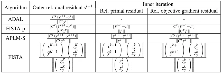
Table 1: Specification of the quantities used in the outer and inner stopping criteria.
that the computation involved in solving the linear systems in those steps was wasted. All of our experiments were performed on a laptop PC with an Intel Core 2 Duo 2.0 GHz processor and 4 Gb of memory.
5.1 Algorithm Parameters and Termination Criteria
Each algorithm (framework + subroutine)4 required several parameters to be set and termination criteria to be specified. We used stopping criteria based on the primal and dual residuals suggested by Boyd et al. (2010). We specify the criteria for each of the algorithms below, but defer their derivation to Appendix C. The maximum number of outer iterations was set to 500, and the tolerance for the outer loop was set atεout =10−4. The number of inner-iterations was capped at 2000, and
the tolerance at the l-th outer iteration for the inner loops wasεlin. Our termination criterion for the outer iterations was
max{rl,sl} ≤εout,
where rl = maxkCxl−ylk
{kCxlk,kylk} is the outer relative primal residual and sl is the relative dual residual, which is given for each algorithm in Table 1. Recall that K+1 is the index of the last inner iteration of the l-th outer iteration; for example, for APLM-S,(xl+1,yl+1)takes the value of the last inner iterate (xK+1,y¯K+1). We stopped the inner iterations when the maximum of the relative primal residual and the relative objective gradient for the inner problem was less thanεlin. (See Table 1 for the expressions of these two quantities.) We see there that sl+1 can be obtained directly from the relative gradient residual computed in the last inner iteration of the l-th outer iteration.
We set µ0=0.01 in all algorithms except that we set µ0=0.1 in ADAL for the data sets other than the first synthetic set and the breast cancer data set. We setρ=µ in FISTA-p and APLM-S and ρ0=µ in FISTA.
For Theorem 1 to hold, the solution returned by the function ApproxAugLagMin(x,y,v)has to become increasingly more accurate over the outer iterations. However, it is not possible to evaluate the sub-optimality quantityαlin (6) exactly because the optimal value of the augmented Lagrangian
L
(x,y,vl)is not known in advance. In our experiments, we used the maximum of the relative primaland dual residuals(max{rl,sl})as a surrogate toαlfor two reasons: First, it has been shown (Boyd et al., 2010) that rl and sl are closely related to αl. Second, the quantities rl and sl are readily available as bi-products of the inner and outer iterations. To ensure that the sequence{εlin}satisfies (6), we basically set:
εl+1
in =βinεlin, (30)
with ε0in=0.01 and βin=0.5. However, since we terminate the outer iterations at εout >0, it is
not necessary to solve the subproblems to an accuracy much higher than the one for the outer loop. On the other hand, it is also important forεlin to decrease to belowεout, since sl is closely related
to the quantities involved in the inner stopping criteria. Hence, we slightly modified (30) and used εl+1
in =max{βinεinl ,0.2εout}.
Recently, we became aware of an alternative ‘relative error’ stopping criterion (Eckstein and Silva, 2012) for the inner loops, which guarantees convergence of Algorithm 2. In our context, this criterion essentially requires that the absolute dual residual is less than a fraction of the absolute primal residual. For FISTA-p, for instance, this condition requires that the(l+1)-th iterate satisfies
2
w0x−xl+1 wly−yl+1
¯
sl+1+(s¯
l+1)2 µ2 ≤σ(¯r
l+1)2,
where ¯r and ¯s are the numerators in the expressions for r and s respectively, σ=0.99, w0x is a constant, and wyis an auxiliary variable updated in each outer iteration by wly+1=wly−µ12CT(y¯K+1− zK). We experimented with this criterion but did not find any computational advantage over the heuristic based on the relative primal and dual residuals.
5.2 Strategies for Updating µ
The penalty parameter µ in the outer augmented Lagrangian (5) not only controls the infeasibility in the constraint Cx=y, but also serves as the step-length in the y-subproblem (and the x-subproblem in the case of FISTA). We adopted two kinds of strategies for updating µ. The first one simply kept µ fixed. In this case, choosing an appropriate µ0 was important for good performance. This was especially true for ADAL in our computational experiments. Usually, a µ0 in the range of 10−1to 10−3worked well.
The second strategy is a dynamic scheme based on the values rland sl(Boyd et al., 2010). Since 1
µpenalizes the primal infeasibility, a small µ tends to result in a small primal residual. On the other
hand, a large µ tends to yield a small dual residual. Hence, to keep rland sl approximately balanced in each outer iteration, our scheme updated µ as follows:
µl+1←
max{βµl,µmin}, if rl>τsl
min{µl/β,µmax}, if sl>τrl
µl, otherwise,
where we set µmax=10, µmin=10−6, τ=10 andβ=0.5, except for the first synthetic data set,
where we setβ=0.1 for ADAL, FISTA-p, and APLM-S.
5.3 Synthetic Examples
The sequence of decision variables x were arranged in groups of ten, with adjacent groups having an overlap of three variables. The support of x was set to the first half of the variables. Each entry in the design matrix A and the non-zero entries of x were sampled from i.i.d. standard Gaussian distributions, and the output b was set to b=Ax+ε, where the noiseε∼
N
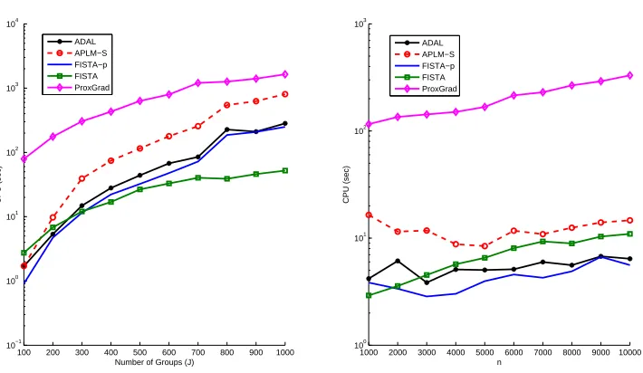
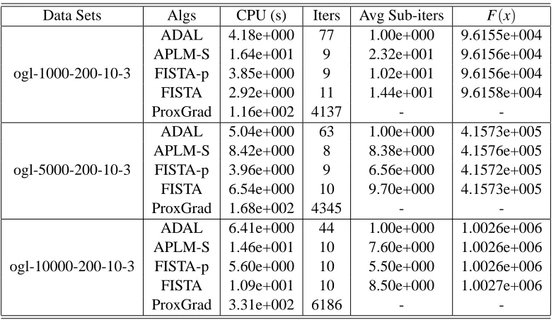
(0,I). Two sets of data were generated as follows: (a) Fix n=5000 and vary the number of groups J from 100 to 1000 with increments of 100. (b) Fix J=200 and vary n from 1000 to 10000 with increments of 1000. The stopping criterion for ProxGrad was the same as the one used for FISTA, and we set its smoothing parameter to 10−3. Figure 1 plots the CPU times taken by the Matlab version of our algorithms and ProxGrad (also in Matlab) on theses scalability tests on l1/l2-regularization. A subset of the numerical results on which these plots are based is presented in Tables 4 and 5.The plots clearly show that the alternating direction methods were much faster than ProxGrad on these two data sets. Compared to ADAL, FISTA-p performed slightly better, while it showed obvious computational advantage over its general version APLM-S. In the plot on the left of Figure 1, FISTA exhibited the advantage of a gradient-based algorithm when both n and m are large. In that case (towards the right end of the plot), the Cholesky factorizations required by ADAL, APLM-S, and FISTA-p became relatively expensive. When min{n,m}is small or the linear systems can be solved cheaply, as the plot on the right shows, FISTA-p and ADAL have an edge over FISTA due to the smaller numbers of inner iterations required.
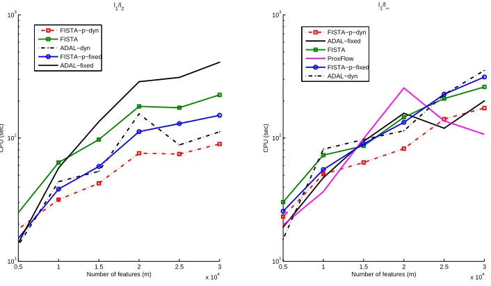
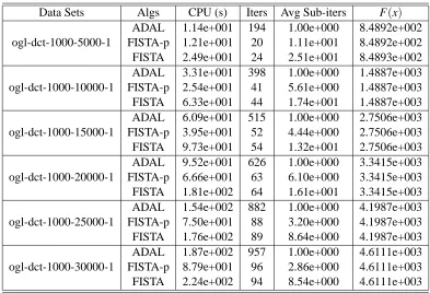
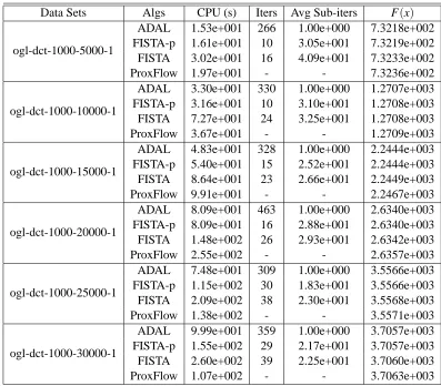
We generated a second data set (dct) using the approach of Mairal et al. (2010) for scalability tests on both the l1/l2 and l1/l∞ group penalties. The design matrix A was formed from over-complete dictionaries of discrete cosine transforms (DCT). The set of groups were all the contiguous sequences of length five in one-dimensional space. x had about 10% non-zero entries, selected randomly. We generated the output as b=Ax+ε, whereε∼
N
(0,0.01kAxk2). We fixed n=1000 and varied the number of features m from 5000 to 30000 with increments of 5000. This set of data leads to considerably harder problems than the previous set because the groups are heavily overlapping, and the DCT dictionary-based design matrix exhibits local correlations. Due to the excessive running time required on Matlab, we ran the C++ version of our algorithms for this data set, leaving out APLM-S and ProxGrad, whose performance compared to the other algorithms is already fairly clear from Figure 1. For ProxFlow, we set the tolerance on the relative duality gap to 10−4, the same asεout, and kept all the other parameters at their default values.Figure 2 presents the CPU times required by the algorithms versus the number of features. In the case of l1/l2-regularization, it is clear that FISTA-p outperformed the other two algorithms. For l1/l∞-regularization, ADAL and FISTA-p performed equally well and compared favorably to ProxFlow. In both cases, the growth of the CPU times for FISTA follows the same trend as that for FISTA-p, and they required a similar number of outer iterations, as shown in Tables 6 and 7. However, FISTA lagged behind in speed due to larger numbers of inner iterations. Unlike in the case of the ogl data set, Cholesky factorization was not a bottleneck for FISTA-p and ADAL here because we needed to compute it only once.
100 200 300 400 500 600 700 800 900 1000 10−1
100 101 102 103 104
Number of Groups (J)
CPU (sec)
ADAL APLM−S FISTA−p FISTA ProxGrad
1000 2000 3000 4000 5000 6000 7000 8000 9000 10000 100
101 102 103
n
CPU (sec)
ADAL APLM−S FISTA−p FISTA ProxGrad
Figure 1: Scalability test results of the algorithms on the synthetic overlapping Group Lasso data sets from Chen et al. (2010). The scale of the y-axis is logarithmic. The dynamic scheme for µ was used for all algorithms except ProxGrad.
however, the dynamic scheme worked well only in the l1/l2case, whereas the performance turned worse in general in the l1/l∞ case. We did not include the results for FISTA with the dynamic scheme because the solutions obtained were considerably more suboptimal than the ones obtained with the fixed-µ scheme. Tables 8 and 9 report the best results of the algorithms in each case. The plots and numerical results show that FISTA-p compares favorably to ADAL and stays competitive to ProxFlow. In terms of the quality of the solutions, FISTA-p and ADAL also did a better job than FISTA, as evidenced in Table 9. On the other hand, the gap in CPU time between FISTA and the other three algorithms is less obvious.
5.4 Real-world Examples
To demonstrate the practical usefulness of our algorithms, we tested our algorithms on two real-world applications.
5.4.1 BREASTCANCERGENEEXPRESSIONS
0.5 1 1.5 2 2.5 3 x 10⁴ 101
102 103
l1/l2
Number of features (m)
CPU (sec)
ADAL FISTA−p FISTA
0.5 1 1.5 2 2.5 3
x 104 101
102 103
l1/l∞
Number of features (m)
CPU (sec)
ADAL FISTA−p FISTA ProxFlow
Figure 2: Scalability test results on the DCT set with l1/l2-regularization (left column) and l1/l∞ -regularization (right column). The scale of the y-axis is logarithmic. All of FISTA-p, FITSA, and ADAL were run with a fixed µ=µ0.
0.5 1 1.5 2 2.5 3
x 104 101
102 103
l 1/l2
Number of features (m)
CPU (sec)
FISTA−p−dyn FISTA ADAL−dyn FISTA−p−fixed ADAL−fixed
0.5 1 1.5 2 2.5 3
x 104 101
102 103
l1/l∞
Number of features (m)
CPU (sec)
FISTA−p−dyn ADAL−fixed FISTA ProxFlow FISTA−p−fixed ADAL−dyn
Data sets N (no. samples) J (no. groups) group size average frequency
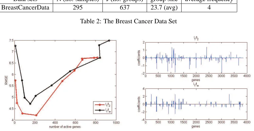
BreastCancerData 295 637 23.7 (avg) 4
Table 2: The Breast Cancer Data Set
Figure 4: On the left: Plot of root-mean-squared-error against the number of active genes for the Breast Cancer data. The plot is based on the regularization path for ten different values for λ. The total CPU time (in Matlab) using FISTA-p was 51 seconds for l1/l2-regularization and 115 seconds for l1/l∞-regularization. On the right: The recovered sparse gene coef-ficients for predicting the length of the survival period. The value ofλused here was the one minimizing the RMSE in the plot on the left.
Table 2 summarizes the data attributes. The numerical results for the l1/l2-norm are collected in Table 10, which show that FISTA-p and ADAL were the fastest on this data set. Again, we had to tune ADAL with different initial values(µ0)and updating schemes of µ for speed and quality of the solution, and we eventually kept µ constant at 0.01. The dynamic updating scheme for µ also did not work for FISTA, which returned a very suboptimal solution in this case. We instead adopted a simple scheme of decreasing µ by half every 10 outer iterations. Figure 6 graphically depicts the performance of the different algorithms. In terms of the outer iterations, APLM-S behaved identically to FISTA-p, and FISTA also behaved similarly to ADAL. However, APLM-S and FISTA were considerably slower due to larger numbers of inner iterations.
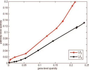
Figure 5: Pathway-level sparsity v.s. Gene-level sparsity.
0 20 40 60 80 100 120 140 2800
3000 3200 3400 3600 3800 4000 4200 4400 4600
Obj value v.s. Iter for BreastCancerData
Outer iters
Obj value
ADAL APLM−S FISTA−p FISTA
0 5 10 15 20 25 30 35 40 45 2800
3000 3200 3400 3600 3800 4000 4200 4400 4600
Obj value v.s. CPU time for BreastCancerData
Log(CPU time) (s)
Obj value
ADAL APLM−S FISTA−p FISTA
Figure 6: Objective values v.s. Outer iters and Objective values v.s. CPU time plots for the Breast Cancer data. The results for ProxGrad are not plotted due to the different objective func-tion that it minimizes. The red (APLM-S) and blue (FISTA-p) lines overlap in the left column.
5.4.2 VIDEOSEQUENCEBACKGROUNDSUBTRACTION
We next considered the video sequence background subtraction task from Mairal et al. (2010) and Huang et al. (2009). The main objective here is to segment out foreground objects in an image (frame), given a sequence of m frames from a fixed camera. The data used in this experiment is available online 5 (Toyama et al., 1999). The basic setup of the problem is as follows. We represent each frame of n pixels as a column vector Aj ∈Rn and form the matrix A∈Rn×m as
A≡ A1 A2 ··· Am
. The test frame is represented by b∈Rn. We model the relationship between b and A by b≈Ax+e, where x is assumed to be sparse, and e is the ’noise’ term which is also assumed to be sparse. Ax is thus a sparse linear combination of the video frame sequence and
accounts for the background present in both A and b. e contains the sparse foreground objects in b. The basic model with l1-regularization (Lasso) is
min
x,e
1
2kAx+e−bk 2+λ(
kxk1+kek1). (31)
It has been shown in Mairal et al. (2010) that we can significantly improve the quality of seg-mentation by applying a group-structured regularization Ω(·) on e, where the groups are all the overlapping k×k-square patches in the image. Here, we set k=3. The model thus becomes
min
x,e
1
2kAx+e−bk
2+λ(kxk
1+kek1+Ω(e)). (32) Note that (32) still fits into the group-sparse framework if we treat the l1-regularization terms as the sum of the group norms, where the each groups consists of only one element.
We also considered an alternative model, where a Ridge regularization is applied to x and an Elastic-Net penalty (Zou and Hastie, 2005) to e. This model
min
x,e
1
2kAx+e−bk 2+λ
1kek1+λ2(kxk2+kek2) (33) does not yield a sparse x, but sparsity in x is not a crucial factor here. It is, however, well suited for our partial linearization methods (APLM-S and FISTA-p), since there is no need for the augmented Lagrangian framework. Of course, we can also apply FISTA to solve (33).
We recovered the foreground objects by solving the above optimization problems and applying the sparsity pattern of e as a mask for the original test frame. A hand-segmented evaluation image from Toyama et al. (1999) served as the ground truth. The regularization parametersλ,λ1, andλ2 were selected in such a way that the recovered foreground objects matched the ground truth to the maximum extent.
FISTA-p was used to solve all three models. The l1model (31) was treated as a special case of the group regularization model (32), with each group containing only one component of the feature vector.6 For the Ridge/Elastic-Net penalty model, we applied FISTA-p directly without the outer augmented Lagrangian layer.
The solutions for the l1/l2,l1/l∞, and Lasso models were not strictly sparse in the sense that those supposedly zero feature coefficients had non-zero (albeit extremely small) magnitudes, since we enforced the linear constraints Cx=y through an augmented Lagrangian approach. To obtain sparse solutions, we truncated the non-sparse solutions using thresholds ranging from 10−9to 10−3 and selected the threshold that yielded the best accuracy.
Note that because of the additional feature vector e, the data matrix is effectively ˜A= A In
∈
Rn×(m+n). For solving (32), FISTA-p has to solve the linear system
ATA+1µDx AT
A In+1µDe
!
x e
=
rx
re
,
where D is a diagonal matrix, and Dx,De,rx,re are the components of D and r corresponding to x
and e respectively. In this example, n is much larger than m, for example, n=57600,m=200. To
6. We did not use the original version of FISTA to solve the model as an l1-regularization problem because it took too
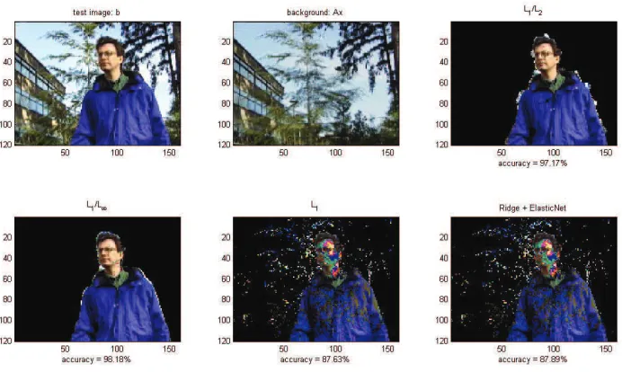
Figure 7: Separation results for the video sequence background substraction example. Each training image had 120×160 RGB pixels. The training set contained 200 images in sequence. The accuracy indicated for each of the different models is the percentage of pixels that matched the ground truth.
avoid solving a system of size n×n, we took the Schur complement of In+1µDeand solved instead
the positive definite m×m system
ATA+1 µDx−A
T(I+1
µDe) −1A
x = rx−AT(I+
1 µDe)
−1r
e,
e = diag(1+1 µDe)
−1(r
e−Ax).
The l1/l∞ model yielded the best background separation accuracy (marginally better than the l1/l2 model), but it also was the most computationally expensive. (See Table 3 and Figure 7.) Although the Ridge/Elastic-Net model yielded as poor separation results as the Lasso (l1) model, it was orders of magnitude faster to solve using FISTA-p. We again observed that the dynamic scheme for µ worked better for FISTA-p than for ADAL. For a constant µ over the entire run, ADAL took at least twice as long as FISTA-p to produce a solution of the same quality. A typical run of FISTA-p on this problem with the best selectedλtook less than 10 outer iterations. On the other hand, ADAL took more than 500 iterations to meet the stopping criteria.
5.5 Comments on Results
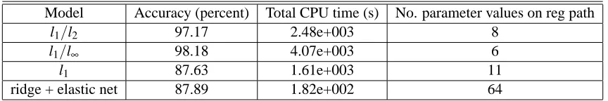
Model Accuracy (percent) Total CPU time (s) No. parameter values on reg path
l1/l2 97.17 2.48e+003 8
l1/l∞ 98.18 4.07e+003 6
l1 87.63 1.61e+003 11
ridge + elastic net 87.89 1.82e+002 64
Table 3: Computational results for the video sequence background subtraction example. The algo-rithm used is FISTA-p. We used the Matlab version for the ease of generating the images. The C++ version runs at least four times faster from our experience in the previous exper-iments. We report the best accuracy found on the regularization path of each model. The total CPU time is recorded for computing the entire regularization path, with the specified number of different regularization parameter values.
data and the breast cancer data, which means that APLM-S essentially behaved like ISTA-p in these cases. Indeed, FISTA-p generally required the same number of outer-iterations as APLM-S but much fewer inner-iterations, as predicted by theory. In addition, no computational steps were wasted and no function evaluations were required for p and ADAL. Second, FISTA-p converged faster (required less iterations) than its full-linearization counterFISTA-part FISTA. We have suggested possible reasons for this in Section 3. On the other hand, FISTA was very effective for data both of whose dimensions were large because it required only gradient computations and soft-thresholding operations, and did not require linear systems to be solved.
Our experiments showed that the performance of ADAL (as well as the quality of the solution that it returned) varied a lot as a function of the parameter settings, and it was tricky to tune them optimally. In contrast, FISTA-p exhibited fairly stable performance for a simple set of parameters that we rarely had to alter and in general performed better than ADAL.
It may seem straight-forward to apply FISTA directly to the Lasso problem (31) without the augmented Lagrangian framework.7 However, as we have seen in our experiments, FISTA took much longer than AugLag-FISTA-p to solve this problem. We believe that this is further evidence of the ‘load-balancing’ property of the latter algorithm that we discussed in Section 3.2. It also demonstrates the versatility of our approach to regularized learning problems.
6. Conclusion
We have built a unified framework for solving sparse learning problems involving group-structured regularization, in particular, the l1/l2- or l1/l∞-regularization of arbitrarily overlapping groups of variables. For the key building-block of this framework, we developed new efficient algorithms based on alternating partial-linearization/splitting, with proven convergence rates. In addition, we have also incorporated ADAL and FISTA into our framework. Computational tests on several sets of synthetic test data demonstrated the relative strength of the algorithms, and through two real-world applications we compared the relative merits of these structured sparsity-inducing norms. Among the algorithms studied, FISTA-p and ADAL performed the best on most of the data sets, and FISTA
appeared to be a good alternative choice for large-scale data. From our experience, FISTA-p is easier to configure and is more robust to variations in the algorithm parameters. Together, they form a flexible and versatile suite of methods for group-sparse problems of different sizes.
Acknowledgments
We would like to thank Katya Scheinberg and Shiqian Ma for many helpful discussions, and Xi Chen for providing the Matlab code for ProxGrad. We also thank the three anonymous reviewers for their valuable suggestions and comments. This research was supported in part by NSF Grant DMS 10-16571, ONR Grant N00014-08-1-1118 and DOE Grant DE-FG02-08ER25856.
Appendix A. Proof of Lemma 1
F(x¯,y¯)−F(x,q¯) ≥ F(x¯,y¯)−
L
ρ(x,y,q¯,∇yf(x,y))= F(x¯,y¯)−
f(x,y) +∇yf(x,y)T(q¯−y) +
1
2ρkq¯−yk
2+g(q¯)
. (34)
From the optimality of ¯q, we also have
γg(q¯) +∇yf(x,y) +
1
ρ(q¯−y) =0. (35)
Since F(x,y) = f(x,y) +g(y), and f and g are convex functions, for any(x¯,y¯),
F(x¯,y¯)≥g(q¯) + (y¯−q¯)Tγg(q¯) +f(x,y) + (y¯−y)T∇yf(x,y) + (x¯−x)T∇xf(x,y). (36)
Therefore, from (34), (35), and (36), it follows that
F(x¯,y¯)−F(x,q¯) ≥ g(q¯) + (y¯−q¯)Tγg(q¯) +f(x,y) + (y¯−y)T∇yf(x,y)
+(x¯−x)T∇xf(x,y)
−
f(x,y) +∇yf(x,y)T(q¯−y) +
1
2ρkq¯−yk
2+g(q¯)
= (y¯−q¯)T(γg(q¯) +∇yf(x,y))−
1
2ρkq¯−yk 2+ (x¯
−x)T∇xf(x,y)
= (y¯−q¯)T
−1ρ(q¯−y)
−21ρkq¯−yk2+ (x¯−x)T∇xf(x,y)
= 1
2ρ(kq¯−y¯k
2− ky−y¯k2) + (x¯−x)T∇
xf(x,y).
The proof for the second part of the lemma is very similar, but we give it for completeness.
F(x,y)−F(p,q)≥F(x,y)−
f(p,q) +g(y¯) +γg(y¯)T(q−y¯) +
1
2ρkq−y¯k 2
(37)
By the optimality of(p,q), we have
∇xf(p,q) = 0, (38)
∇yf(p,q) +γg(y¯) +
1