Revisiting Stein’s Paradox: Multi-Task Averaging
Sergey Feldman sergey.feldman@gmail.com
Data Cowboys 9126 23rd Ave. NE Seattle, WA 98115, USA
Maya R. Gupta mayagupta@google.com
1225 Charleston Rd
Mountain View, CA 94301, USA
Bela A. Frigyik frigyik@gmail.com
Institute of Mathematics and Informatics University of P´ecs
H-7624 P´ecs, Ifj´us´ag St. 6, Hungary
Editors:Ben Taskar, Massimiliano Pontil
Abstract
We present a multi-task learning approach to jointly estimate the means of multiple inde-pendent distributions from samples. The proposed multi-task averaging (MTA) algorithm results in a convex combination of the individual task’s sample averages. We derive the op-timal amount of regularization for the two task case for the minimum risk estimator and a minimax estimator, and show that the optimal amount of regularization can be practically estimated without cross-validation. We extend the practical estimators to an arbitrary number of tasks. Simulations and real data experiments demonstrate the advantage of the proposed MTA estimators over standard averaging and James-Stein estimation.
Keywords: multi-task learning, James-Stein, Stein’s paradox
1. Introduction
The mean is one of the most fundamental and useful tools in statistics (Salsburg, 2001). By the 16th century Tycho Brahe was using the mean to reduce measurement error in as-tronomical investigations (Plackett, 1958). Legendre (1805) noted that the mean minimizes the sum of squared errors to a set of samples:
¯
y= arg min
˜ y
N X
i=1
(yi−y˜)2. (1)
More recently it has been shown that the mean minimizes the sum of any Bregman di-vergence to a set of samples (Banerjee et al., 2005; Frigyik et al., 2008). Gauss (1857) commented on the mean’s popularity in his time:
same circumstances and with equal care, the arithmetical mean of the observed values affords the most probable value, if not rigorously, yet very nearly at least, so that it is always most safe to adhere to it.”
But the mean is a more subtle quantity than it first appears. In a surprising result popularly called Stein’s paradox (Efron and Morris, 1977), Stein (1956) showed that it is better (in a summed squared error sense) to estimate each of the means of T Gaussian random variables using data sampled from all of them, even if the random variables are independent and have different means. That is, it is beneficial to consider samples from seeminglyunrelated distributions to estimate a mean. Stein’s result is an early example of the motivating hypothesis behind multi-task learning: that leveraging data from multiple tasks can yield superior performance over learning from each task independently. In this work we consider a multi-task regularization approach to the problem of estimating multiple means; we call this multi-task averaging (MTA).
Multi-task learning is most intuitive when the multiple tasks are conceptually similar. But we argue that it is really thestatistical similarity of the multiple tasks that determines how well multi-task learning works. In fact, a key result of this paper is that proposed multi-task estimation achieves lower total squared error than the sample meanif the true means of the multiple tasks are close compared to the variance of the samples (see Equation 12). Of course, in practice cognitive notions of similarity can be a useful guide for multi-task learning, as tasks that seem similar to humans often do have similar statistics.
We begin the paper with the proposed MTA objective in Section 2, and review related work in Section 3. We show that MTA has provably nice theoretical properties in Section 4; in particular, we derive the optimal notion of task similarity for the two task case, which is also the optimal amount of regularization to be used in the MTA estimation. We generalize this analysis to form practical estimators for the general case of T tasks. Simulations in Section 5 verify the advantage of MTA over standard sample means and James-Stein esti-mation if the true means are close compared to the variance of the underlying distributions. In Section 6 we present four experiments on real data: (i) estimating Amazon customer reviews, (ii) estimating class grades, (iii) forecasting sales, and (iv) estimating the length of kings’ reigns. These real-data experiments show that MTA is generally 10-20% better than the sample mean.
A short version of this paper was published in NIPS 2012 (Feldman et al., 2012). This paper substantially differs from that conference paper that it contains more analysis, proofs, and new and expanded experiments.
2. Multi-Task Averaging
Consider the problem of estimating the means ofT random variables that have finite means
{µt} and variances {σt2} for t = 1, . . . , T. We treat this as a T-task multi-task learning
problem, and estimate theTmeans jointly. We take as givenNtindependent and identically
distributed (iid) random samples {Yti}Ni=1t for each taskt. Key notation is summarized in
T number of tasks
Nt number of samples fortth task
µt true mean of taskt
σt2 variance of the tth task
Yti∈R ith random sample from tth task
¯
Yt∈R sample average fortth task: N1t P
iYti,
also referred to as the single-task mean estimate ¯
Y ∈RT vector withtth component ¯Yt
Yt∗∈R MTA estimate oftth mean Y∗∈RT vector withtth component Y∗
t
ˆ
Yt∈R an estimate of thetth mean
˜
Yt∈R dummy variable
Σ∈RT×T diagonal covariance matrix of ¯Y with Σtt= σ 2 t Nt
A∈RT×T pairwise task similarity matrix
L=D−A graph Laplacian of A, with diagonal Ds.t. Dtt=PTr=1Atr
W MTA solution matrix, W = (I+TγΣL)−1
Table 1: Key Notation
In this paper, we judge the estimates by total squared error: given T estimates {Yˆt}
and T true means {µt}:
estimation error({Yˆt)})
4 = T X t=1
µt−Yˆt 2
, (2)
Equivalently (up to an additive factor), the metric can be expressed as the total squared expected error to a random sample Yt from each task:
regression error({Yˆt)})
4 = T X t=1 E
Yt−Yˆt 2
; (3)
we use an empirical approximation to (3) in the experiments because the true means are not known but held-out samples from the distributions are available.
Let a T×T matrix A describe the relatedness or similarity of any pair of theT tasks, with Att = 0 for all t without loss of generality (because the diagonal self-similarity terms
are canceled in the objective below). Further we assume each task’s variance σt2 is known or already estimated. The proposed MTA objective is
{Yt∗}Tt=1= arg min {Y˜t}T
t=1 1 T T X t=1 Nt X i=1
(Yti−Y˜t)2
σt2 +
γ T2 T X r=1 T X s=1
Ars( ˜Yr−Y˜s)2. (4)
by tying them together. The regularization parameterγ balances the empirical risk and the multi-task regularizer. Ifγ = 0, the MTA objective decomposes into T separate minimiza-tion problems, producing the sample averages{Y¯t}. Ifγ = 1, the balance between empirical
risk and multi-task regularizer is completely specified by the task similarity matrixA. A more general formulation of MTA is
{Yt∗}Tt=1 = arg min {Y˜t}T
t=1
1 T
T X
t=1 Nt X
i=1
L(Yti,Y˜t) +γJ
{Y˜t}Tt=1
,
where L is some loss function and J is some regularization function. If L is chosen to be any Bregman loss, then settingγ = 0 will produce theT sample averages (Banerjee et al., 2005). For the analysis and experiments in this paper, we restrict our focus to the tractable squared-error formulation given in (4). The MTA objective and many of the results in this paper generalize straightforwardly to samples that are vectors rather than scalars (see Section 4.2), but for most of the paper we restrict our focus to scalar samples Yti∈R.
The task similarity matrix A can be specified as side information, for example from a domain expert, but often this side information is not available, or it may not be clear how to convert semantic notions of task similarity into appropriate numerical values for the task-similarity values in A. In such cases, A can be treated as a matrix parameter of the MTA objective, and in Section 4 we fix γ = 1 and derive two optimal choices of A for the T = 2 case: the A that minimizes expected squared error, and a minimax A. We use the T = 2 analysis to propose practical estimators ofAfor any number of tasks, removing the need to cross-validate the amount of regularization.
3. Related Work
In this section, we review related and background material: James-Stein estimation, multi-task learning, manifold regularization, and the graph Laplacian.
3.1 James-Stein Estimation
A closely related body of work to MTA is Stein estimation (James and Stein, 1961; Bock, 1975; Efron and Morris, 1977; Casella, 1985), which can be derived as an empirical Bayes strategy for estimating multiple means simultaneously (Efron and Morris, 1972). James and Stein (1961) showed that the maximum likelihood estimate of the task mean can be dominated by a shrinkage estimate given Gaussian assumptions. Specifically, given a single sample drawn from T normal distributions Yt ∼ N(µt, σ2) for t = 1, . . . , T, Stein showed
that the maximum likelihood estimator ¯Yt = Yt is inadmissible, and is dominated by the
James-Stein estimator:
ˆ YtJ S =
1−(T−2)σ 2
¯ Y>Y¯
¯
Yt, (5)
where ¯Y is a vector withtth entry ¯Yt. The above estimator dominates ¯Yt whenT >2. For
Note that in (5) the James-Stein estimatorshrinks the sample means towards zero (the terms “regularization” and “shrinkage” are often used interchangeably). The form of (5) and its shrinkage towards zero points to the implicit assumption that theµt are themselves
drawn from a standard normal distribution centered at 0. More generally, the means are assumed to be drawn as µt∼ N(ξ,1). The James-Stein estimator then becomes
ˆ
YtJ S =ξ+
1− (T −3)σ 2
( ¯Y −ξ1)>( ¯Y −ξ1)
( ¯Yt−ξ), (6)
where ξ can be estimated (as we do in this work) as the average of means ξ = ¯Y¯ =
1 T
PT
r=1Y¯r, and this additional estimation decreases the degrees of freedom by one.1 Note
that (6) shrinks the estimates towards the mean-of-meansξ rather than shrinking towards zero. Also, the more similar the multiple tasks are (in the sense that individual task means are closer to the mean-of-meansξ), the more regularization occurs in (6).
There have been a number of extensions to the original James-Stein estimator. The James-Stein estimator given in (6) is itself not admissible, and is dominated by the positive part James-Stein estimator (Lehmann and Casella, 1998), which was further theoretically improved by Bock’s James-Stein estimator (Bock, 1975). Throughout this work, we compare to Bock’s well-regarded positive-part James-Stein estimator for multiple data points per task and independent unequal variances (Bock, 1975; Lehmann and Casella, 1998). In particular, letYti∼ N(µt, σt2) for t= 1, . . . , T and i= 1, . . . , Nt, let Σ be the covariance matrix of the
vector of task sample means ¯Y, and let λmax(Σ) be the largest eigenvalue of Σ, then the
estimator is
ˆ
YtJ S =ξ+
1−
tr(Σ)
λmax(Σ)−3
( ¯Y −ξ1)>Σ−1( ¯Y −ξ1)
+
( ¯Yt−ξ), (7)
where (x)+ = max(0, x).
3.2 Multi-Task Learning for Mean Estimation
MTA is an approach to the problem of estimating T means. We are not aware of other work in the multi-task literature that addresses this problem explicitly; most multi-task learning methods are designed for regression, classification, or feature selection, for example, Micchelli and Pontil (2004); Bonilla et al. (2008); Argyriou et al. (2008). Estimating T means can be considered a special case of multi-task regression, where one fits a constant function to each task, since, with a feature space of zero dimensions only the constant offset term is learned. And, similarly to MTA, one of the main approaches to multi-task regression in the literature is tying tasks together with an explicit multi-task parameter regularizer.
Abernethy et al. (2009), for instance, propose to minimize the empirical loss by adding the regularizer
||β||∗,
where thetth column of the matrixβ is the vector of parameters for thetth task and||·||∗is the trace norm. Applying this approach to mean estimation, the matrixβhas only one row,
1. For more details as to whyT−2 in (5) becomesT−3 in (6), see Example 7.7 on page 278 of Lehmann
and ||β||∗ reduces to the`2 norm on the outputs, thus for mean estimation this regularizer
does not actually tie the tasks together.
Argyriou et al. (2008) propose a a different regularizer,
tr(β>D−1β),
where Dis a learned, shared feature covariance matrix. With no features (as in the MTA application of constant function regression),Dis just a constant andtr(β>D−1β) is a ridge regularizer on the outputs. The regularizers in the work of Jacob et al. (2008) and Zhang and Yeung (2010) reduce similarly when applied to mean estimation. These regularizers are similar to theoriginalJames Stein estimator in that they shrink the estimates towards zero; though more modern James Stein estimators shrink towards a pooled mean (see Section 3.1).
The most closely related work is that of Sheldon (2008) and Kato et al. (2008), where the regularizer or constraint, respectively, is
T X
r=1 T X
s=1
Arskβr−βsk22,
which is the MTA regularizer if applied to mean estimation. In this paper we do just that: apply this regularizer to mean estimation, show that this special case enables new and useful analytic results, and demonstrate its performance with simulated and real data.
3.3 Multi-Task Learning and the Similarity Between Tasks
A key issue for MTA and many other multi-task learning methods is how to estimate some notion of similarity (or task relatedness) between tasks and/or samples if it is not provided. A common approach is to estimate the similarity matrix jointly with the task parameters (Argyriou et al., 2007; Xue et al., 2007; Bonilla et al., 2008; Jacob et al., 2008; Zhang and Yeung, 2010). For example, Zhang and Yeung (2010) assume that there exists a covariance matrix for the task relatedness, and proposed a convex optimization approach to estimate the task covariance matrix and the task parameters in a joint, alternating way. Applying such joint and alternating approaches to the MTA objective given in (4) leads to a degenerate solution with zero similarity. However, the simplicity of MTA enables us to specify the optimal task similarity matrix forT = 2 (see Section 4), which we use to obtain closed-form estimators for the general T >1 case.
3.4 Manifold Regularization
MTA is similar in form tomanifold regularization (Belkin et al., 2006). For example, Belkin et al.’s Laplacian-regularized least squares objective for semi-supervised regression solves
arg min
f∈H
PN
i=1(yi−f(xi))2+λ||f||2H+γ
PN+M
i,j=1 Aij(f(xi)−f(xj))2,
xi and xj, and ||f||H is the norm of the function f in the RKHS. In MTA, as opposed to manifold regularization, we are estimating a different function (that is, the constant function that is the mean) for each of theT tasks, rather than a single global function. One can interpret MTA as regularizing the individual task estimates over the task-similarity manifold, which is defined for theT tasks by the T×T matrixA.
3.5 Background on the Graph Laplacian Matrix
It will be helpful for later sections to review the graph Laplacian matrix. For graph G with T nodes, let A ∈ RT×T be a matrix where component Ars ≥ 0 is the weight of the
edge between node r and node s, for all r, s. The graph Laplacian matrix is defined as L=L(A) =D−A, with diagonal matrixD such thatDtt=PsAts.
The graph Laplacian matrix is analogous to the Laplacian operator, which quantifies how locally smooth a twice-differentiable function g(x) is. Similarly, the graph Laplacian matrix L can be thought of as being a measure of the smoothness of a function defined on a graph. Given a function f defined over the T nodes of graph G, where fi ∈ Ris the
function value at node i, the totalenergy of a graph is (for symmetricA)
E(f) = 1 2
T X
i=1 T X
j=1
Aij(fi−fj)2 =f>L(A)f,
which is small whenf is smooth over the graph (Zhu and Lafferty, 2005). IfAis asymmetric then the energy can be written as
E(f) = 1 2
T X
i=1 T X
j=1
Aij(fi−fj)2 =f>L((A+A>)/2)f. (8)
When each fi ∈ Rd is a vector, one can alternatively write the energy in terms of the
distance matrix:
E(f) = 1 2tr(∆
>A),
where ∆ij = (fi−fj)>(fi−fj).
As discussed above, the graph Laplacian can be thought of as an operator on a func-tion, but it is useful in and of itself (i.e., without a function). The eigenvalues of the graph Laplacian are all real and non-negative, and there is a wealth of literature showing how the eigenvalues reveal the structure of the underlying graph and can be used for clustering (v. Luxburg, 2007). The graph Laplacian is a common tool in semi-supervised learning lit-erature (Zhu and Goldberg, 2009), and the Laplacian of a random walk probability matrix P (i.e., all the entries are non-negative and the rows sum to 1) is also of interest. For exam-ple, Saerens et al. (2004) showed that the pseudo-inverse of the Laplacian of a probability transition matrix is used to compute the square root of the average commute time (the average time taken by a random walker on graphGto reach nodej for the first time when starting at node i, and coming back to node i).
4. MTA Theory and Estimators
First, we give a general closed-form solution for the MTA mean estimates and characterize the MTA objective in Sections 4.1 through 4.3. Then in Section 4.4 we analyze the estima-tion error for the two taskT = 2 case and give conditions for when MTA is better than the sample means. In Section 4.5, we derive the optimal similarity matrix A for the two task case.
Then in Section 4.7, we generalize our T = 2 analysis to propose practical estimators for any number of tasks T, and analyze their computational efficiency. In Section 4.8, we analyze the relationship of different estimators formed by linearly combining the sample means, including the MTA estimators, James Stein, and other estimators that regularize sample means towards a pooled mean. Lastly, we discuss the Bayesian interpretation of MTA in Section 4.9.
Proofs and derivations are in the appendix.
4.1 Closed-form MTA Solution
Without loss of generality, we only deal with symmetricAbecause in the case of asymmetric A it is equivalent to consider instead the symmetrized matrix (A>+A)/2.
For symmetricAwith non-negative components, the MTA objective given in (4) is con-tinuous, differentiable, and convex; and (4) has closed-form solution (derivation in Appendix A):
Y∗ =
I+ γ
TΣL
−1
¯
Y , (9)
where ¯Y is the vector of sample averages with tth entry ¯Yt = N1t PNi=1t Yti, L is the graph
Laplacian ofA, and Σ is the diagonal covariance matrix of the sample mean vector ¯Y such that Σtt = σ
2 t
Nt. The inverse I+ γ TΣL
−1
in (9) always exists:
Lemma 1 Suppose that 0 ≤Ars <∞ for all r, s, γ ≥0, and 0 < σ 2 t
Nt <∞ for all t. The MTA solution matrix W = I+TγΣL−1
exists.
The MTA estimates Y∗ converge to the vector of true meansµ:
Proposition 2 As Nt→ ∞ ∀ t, Y∗ →µ.
4.2 MTA for Vectors
MTA can also be applied to vectors. Let Y∗ ∈ RT×d be a matrix with Yt∗ as its tth row
and let ¯Y∈RT×d be a matrix with ¯Yt ∈Rd as itstth row. One can perform MTA on the
vectorized form of Y∗:
vec(Y∗) =
I+ γ
TΣL
−1
vec( ¯Y),
4.3 Convexity of MTA Solution
One sees from (9) that the MTA estimates are linear combinations of the sample averages:
Y∗=WY ,¯ whereW =I+ γ
TΣL
−1
.
Moreover, and less obviously, each MTA estimate is aconvex combination of the single-task sample averages:
Theorem 3 If γ ≥0, 0≤Ars <∞ for all r, s and 0< σ 2 t
Nt < ∞ for all t, then the MTA estimates {Yt∗} given in (9) are convex combinations of the task sample averages {Y¯t}.
This theorem generalizes a result of Chebotarev and Shamis (2006) that the matrix (I +γL)−1 is right-stochastic (i.e., the rows are non-negative and sum to 1) if the entries ofA are strictly positive. Our proof (given in the appendix) uses a different approach, and extends the result both to the more general form of the MTA solution matrix I+ TγΣL−1 and to A with non-negative entries.
4.4 MSE Analysis for the Two Task Case
In this section we analyze the T = 2 task case, with N1 and N2 samples for tasks 1 and
2 respectively. Suppose random samples drawn for the first task {Y1i} are iid with finite
mean µ1 and finite variance σ12, and random samples drawn for the second task {Y2i} are
iid with finite meanµ2=µ1+ ∆ and finite varianceσ22. Let the task-relatedness matrix be
A= [0 a;a0], and without loss of generality, we fix γ = 1. Then the closed-form solution (9) can be simplified:
Y1∗ =
2 + σ22 N2a
2 + σ12 N1a+
σ2 2 N2a
Y¯1+
σ2 1 N1a
2 + σ12 N1a+
σ2 2 N2a
Y¯2. (10)
The mean squared error of Y1∗ is
MSE[Y1∗] = σ
2 1 N1
4 + 4σ22 N2a+
σ2 1σ22 N1N2a2+
σ4 2 N2 2a 2
2 + σ21 N1a+
σ2 2 N2a 2 +
∆2σ41 N2
1a 2
2 + σ12 N1a+
σ2 2 N2a
2. (11)
Next, we compare the MTA estimateY1∗ to the sample average ¯Y1, which is the maximum
likelihood estimate of the true meanµ1 for many distributions.2 The MSE of the single-task
sample average ¯Y1 is σ 2 1
N1, and comparing that to (11) and simplifying some tedious algebra
establishes that
MSE[Y1∗]<MSE[ ¯Y1] if ∆2 <
4
a+
σ21 N1 + σ 2 2 N2 . (12)
Thus the MTA estimate of the first mean has lower MSE than the sample average estimate if the squared mean-separation ∆2is small compared to the summed variances of the sample
means. See Figure 1 for an illustration.
2. The uniform distribution is perhaps the simplest example where the sample average isnot the maximum
0 0.5 1 1.5 2 2.5 −30
−20 −10 0 10 20 30
mean of the second task
% change in risk vs. single−task
Single−Task MTA, N = 2 MTA, N = 10 MTA, N = 20
Figure 1: Plot shows the percent change in average risk for two tasks (averaged over 10,000 runs of the simulation). For each task there areN iid samples, forN = 2,10,20. The first task generates samples from a standard Gaussian. The second task generates samples from a Gaussian withσ2 = 1 and different mean value, which is varied as marked on the x-axis. The symmetric task-relatedness value was fixed at a = 1 (note this is generally not the optimal value). One sees that given N = 2 samples from each Gaussian, the MTA estimate is better than the single-task sample if the difference between the true means is less than 1.5. Given N = 20 samples from each Gaussian, the MTA estimate is better if the distance between the means is less than 2. In the extreme case that the two Gaussians have the same mean (µ1 = µ2 = 0), then even with this suboptimal choice of
a= 1, MTA provides a 20% win for N = 2 samples, and a 5% win for N = 20 samples.
Further, because of the symmetry of (12), if the condition of (12) holds, it is also true that MSE[Y2∗]<MSE[ ¯Y2], such that the MSE of each task individually is reduced.
The condition (12) shows that even when the true means are far apart such that ∆ is large, there is some tiny amount of MTA regularization athat will improve the estimates.
4.5 Optimal Task Relatedness A for T = 2
We analyze the optimal choice ofain the task-similarity matrix A= [0a;a0]. The risk is the sum of the mean squared errors:
R(µ, Y∗) = MSE[Y1∗] + MSE[Y2∗], (13)
0 2 4 6 8 10 0
0.2 0.4 0.6 0.8 1
task relatedness value
risk
MTA, N = 2 MTA, N = 10 MTA, N = 20
Figure 2: Plot shows the risk for two tasks, where the task samples were drawn iid from GaussiansN(0,1) andN(1,1). The task-relatedness valueawas varied as shown on the x-axis. The minimum expected squared error is marked by a dot, and occurs for the choice ofagiven by (14), and is independent ofN.
Minimizing (13) w.r.t. aone obtains the optimal:
a∗ = 2
∆2, (14)
which is always non-negative, as was assumed. This result is key because it specifies that the optimal task-similaritya∗ ideally should measure the inverse of the squared task mean-difference. Further, the optimal task-similarity is independent of the number of samplesNt
or the sample varianceσt2, as these are accounted for in Σ of the MTA objective. Note that a∗ also minimizes the functions MSE[Y1∗] and MSE[Y2∗], separately.
The effect on the risk on the choice of aand the optimala∗ is illustrated in Figure 2. Analysis of the second derivative shows that this minimizer always holds forN1, N2 ≥1.
In the limit case, when the difference in the task means ∆ goes to zero (while σ2 t stay
constant), the optimal task-relatedness a∗ goes to infinity, and the weights in (10) on ¯Y1
and ¯Y2 become 1/2 each.
4.6 Estimating Task Similarity from Data for T = 2 Tasks
The optimal two-task similarity given in (14) requires knowledge of the true means µ1
and µ2. These are, in practice, unavailable. What similarity should be used then? A
straightforward approach is to use single-task estimates instead:
ˆ
a∗= 2
(¯y1−y¯2)2
and to use maximum likelihood estimates ˆσt2to form the matrix ˆΣ. This data-dependent ap-proach is analogous to empirical Bayesian methods in which prior parameters are estimated from data (Casella, 1985).
4.7 Estimating Task Similarity from Data for Arbitrary T Tasks
Based on our analysis in the preceding sections of the optimalA for the two-task case, we propose two methods to estimate A from data for arbitrary T > 1. The first method is designed to minimize the approximate risk using a constant similarity matrix. The second method provides a minimax estimator. With both methods one can take advantage of the Sherman-Morrison formula (Sherman and Morrison, 1950) to avoid taking the matrix inverse or solving a set of linear equations in (9) (detailed in Section 4.7.3). For the special case that all task variances are assumed equal (an assumption used in all of our experiments), the computation time isO(T).
4.7.1 MTA Constant
The risk of estimator ˆY =WY¯ is
R(µ, WY¯) =E[(WY¯ −µ)>(WY¯ −µ)] (15)
=tr(WΣW>) +µ>(I−W)>(I−W)µ, (16)
where (16) uses the fact that E[ ¯YY¯>] =µµ>+ Σ.
One approach to generalizing the results of Section 4.4 to arbitrary T is to try to find a symmetric, non-negative matrix A such that the (convex, differentiable) risk R(µ, WY¯) is minimized for W = I+TγΣL−1
(recall L is the graph Laplacian of A). The problem with this approach is two-fold: (i) the solution is not analytically tractable forT > 2 and (ii) an arbitraryA hasT(T−1) degrees of freedom, which is considerably more than theT means we are trying to estimate in the first place. To avoid these problems, we generalize the two-task results by constraining A to be a scaled constant matrix A=a11>, and find the optimal a∗ that minimizes the risk given by (16). As in Section 4.4, we fix γ = 1. For analytic tractability, we add the assumption that all the Yt have the same variance,
estimating Σ as trT(Σ)I. Then minimizing (15) becomes:
a∗ = arg min
a
R µ,
I+ 1
T
tr(Σ)
T L(a11
>)
−1
¯ Y
!
,
which has the solution
a∗ = 1 2
T(T−1) PT
r=1 PT
s=1(µr−µs)2
, (17)
which does reduce to the optimal two task MTA solution (14) whenT = 2.
While (17) is theoretically interesting, in practice, one of course does not have {µr} as
these are precisely the values one is trying to estimate, and thus cannot use (17) directly. Instead, we propose estimatinga∗ using the sample means {y¯r}:
ˆ
a∗ = 2
1 T(T−1)
PT r=1
PT
s=1(¯yr−y¯s)2
Using the optimal estimated constant similarity given in (18) and an estimated covari-ance matrix ˆΣ produces what we refer to as the MTA Constant estimate
Y∗ =
I+ 1
TΣˆL(ˆa
∗11>)
−1
¯
Y . (19)
Note that we made the assumption that the entries of Σ were the same in order to be able to derive (17), but we do not need nor necessarily suggest that assumption on the ˆΣ be used in practice with ˆa∗ in (19).
4.7.2 MTA Minimax
Bock’s James-Stein estimator is minimax (Lehmann and Casella, 1998)). In this section, we derive a minimax version of MTA for arbitrary T that prescribes less regularization than MTA Constant. Formally, an estimatorYM ofµis called minimax if it minimizes the
maximum risk:
inf
˜ Y
sup
µ
R(µ,Y˜) = sup
µ
R(µ, YM).
Let r(π,Yˆ) be the average risk of estimator ˆY w.r.t. a prior π(µ) such that r(π,Yˆ) =
R
R(µ,Yˆ)π(µ)dµ. The Bayes estimatorYπ is the estimator that minimizes the average risk, and the Bayes riskr(π, Yπ) is the average risk of the Bayes estimator. A prior distribution π is called least favorable if r(π, Yπ)> r(π0, Yπ0) for all priorsπ0.
First, we will specify MTA Minimax for the T = 2 case. To find a minimax estimator YM it is sufficient to show that (i) YM is a Bayes estimator w.r.t. the least favorable prior (LFP) and (ii) it has constant risk (Lehmann and Casella, 1998). To find a LFP, we first need to specify a constraint set forµt; we use an interval: µt∈[bl, bu],for allt, wherebl∈R
and bu∈R. With this constraint set the minimax estimator is (see appendix for details):
YM =
I+ 2
T(bu−bl)2
ΣL(11>)
−1
¯ Y ,
which reduces to (14) whenT = 2. This minimax analysis is only valid for the case when T = 2, but we found that the following extension of MTA Minimax to largerT worked well in simulations and applications for anyT ≥2. To estimatebu and bl from data we assume
the unknown T means are drawn from a uniform distribution and use maximum likelihood estimates of the lower and upper endpoints for the support:
ˆ
bl = min
t y¯t and ˆbu= maxt y¯t.
Thus, in practice, MTA Minimax is
YM = I+ 2
T(ˆbu−ˆbl)2
ˆ
ΣL(11>)
!−1
4.7.3 Computational Efficiency of MTA Constant and Minimax
Both MTA Constant and MTA Minimax weight matrices can be written as
(I +cΣL(11>))−1 = (I+cΣ(T I−11>))−1 = (I+cTΣ−cΣ11>)−1 = (Z−z1>)−1,
where c is different for MTA Constant and MTA Minimax, Z =I +cTΣ, z =cΣ1. The Sherman-Morrison formula (Sherman and Morrison, 1950) can be used to find the inverse:
(Z−z1>)−1 =Z−1+Z
−1z1>Z−1
1−1>Z−1z.
Since Z is diagonal,Z−1 can be computed in O(T) time, and so canZ−1z.
Further the computation becomesO(T) if the covariance matrix Σ is taken to be diagonal with constant component σ2, an assumption we use in all our experiments. In that case, compute the constant v = 1/(1 +cσ2), and then the MTA estimate reduces to a convex combination of the task sample average and the pooled sample average: vY¯+ (1−v)PT
t Y¯t.
4.8 Generality of MTA
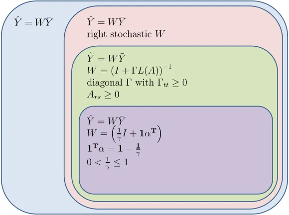
In this section, we use the expression ‘matrices of MTA form’ to refer to matrices that can be written
(I+ ΓL(A))−1, (20)
where A is a matrix with all non-negative entries, and Γ is a diagonal matrix with all non-negative entries. Matrices of the form (I +γL)−1 have been used as graph kernels (Fouss et al., 2006; Yajima and Kuo, 2006), and were termed regularized Laplacian kernels (RLKs) by Smola and Kondor (2003). The RLK assumes that A (and L) are symmetric, and thus MTA and (20) strictly generalizes the RLK because ΓL is only symmetric for some special cases such as when Γ is a scaled identity matrix. Thus, one might also refer to matrices of the form (20) as generalized regularized Laplacian kernels, but in this section we focus on their role as estimators and in understanding relationships with the proposed MTA estimator.
Figure 3 is a Venn diagram of the sets of estimators that can be expressed ˆY = WY¯, where W is some T ×T matrix. The first subset (the pink region) is all estimators where W is right-stochastic. The second subset (the green region) is estimators of MTA form as per (20). The innermost subset (the purple region) includes many well-known estimators such as the James-Stein estimator, and estimators that regularize single-task estimates of the mean to the pooled mean or the average of means. In this section we will prove that the innermost purple subset is astrict subset of the green MTA subset, such that any innermost estimator can be written in MTA form for specific choices of A, γ, and Σ. Note that the covariance Σ is treated as a “choice” because some classic estimators assume Σ =I.
Proposition 4 The set of estimatorsWY¯ where W is of MTA form as per (20) is strictly larger than the set of estimators that regularize the single-task estimates as follows:
ˆ
Y =
1
γI+1α
>
^
Y =WY¹ Y^ =WY¹
right stochasticW
^
Y =WY¹
W = (I+ ¡L(A))¡1 diagonal ¡ with ¡tt¸0 Ars¸0
^
Y =WY¹ W =
³
1 °I+1®
T
´
1T®=1¡1 °
0< 1 ° ·1
Figure 3: A Venn diagram of the set membership properties of various estimators of the type ˆY =WY¯.
where PT
r=1αr= 1−γ1, γ ≥1, andαr≥0,∀r.
Corollary 5 Estimators that regularize the single task estimate towards the pooled mean such that they can be written
ˇ
Yt=λY¯t+
1−λ
PT r=1Nr
T X
s=1 Ns X
i=1
Ysi,
for λ∈(0,1] can also be written in MTA form as
ˇ
Y =
I+ 1−λ
λN>1L(1N >
)
−1
¯ Y ,
where N is a T by 1 vector with Nt as its tth entry since in Proposition 4 we can choose
γ = λ1 and α= N1−Tλ1N, which matches (20) with Γ = 1−λ
λN>1I and A=1N>.
Corollary 6 Estimators which regularize the single task estimate towards the average of means such that they can be written
˘
Yt=λY¯t+
1−λ T
T X
t=1
for λ∈(0,1], can also be written in MTA form as
˘
Y =
I+ 1−λ
λT L(11
> )
−1
¯ Y ,
since in Proposition 4 we can choose γ = 1λ and α = 1−Tλ1, which matches (20) with
Γ = 1λT−λI andA=11>.
Note that the proof of the proposition in the appendix uses MTA form withasymmetric
similarity matrixA. The MTA form with asymmetricAarises if you replace the symmetric MTA regularization term in (4) with the following asymmetric regularization term as follows:
1 2
T X
r=1 T X
s=1
Ars( ˜Yr−Y˜s)2+
1 2
T X
r=1 T X
s=1
Ars !
˜ Yr2−1
2
T X
r=1 T X
s=1
Asr !
˜ Yr2.
Lastly, we make a note about the sum of the mean estimates for the different estimators of Figure 3. In general, the sum of the estimates ˆY =WY¯ for right-stochasticW may differ from the sum of the sample means, because1>WY¯ 6=1>Y¯ for all right-stochasticW. But in the special case of Bock’s positive-part James-Stein estimator the sum is preserved:
Proposition 7
1>YˆJ S =1>Y ,¯ (21)
where YˆJ S is given in (7).
We illustrate this property in the Kings’ reigns experiments in Table 7.
4.9 Bayesian Interpretation of MTA
The MTA estimates from (4) can be interpreted as jointly maximizing the likelihood of T Gaussian distributions with a joint Gaussian Markov random field (GMRF) prior (Rue and Held, 2005) on the solution. In MTA, the precision matrix (the inverse covariance of the GMRF prior) is L, the graph Laplacian of the similarity matrix, and is thus positive semi-definite (and not strictly positive definite); GMRFs with PSD inverse covariances are called intrinsic GMRFs (IGMRFs).
GMRFs and IGMRFs are commonly used in graphical models, wherein the sparsity structure of the precision matrix (which corresponds to conditional independence between variables) is exploited for computational tractability. Because MTA allows for arbitrary but non-negative similarities between any two tasks, the precision matrix does not (in general) have zeros on the off-diagonal, and it is not obvious how additional sparsity structure of L would be of help computationally.
Additionally, none of the results we show in this paper require a Gaussian assumption nor any other assumption about the parametric form of the underlying distribution.
5. Simulations
first with simulations, then with real data. In these sections we use lower-case notation to indicate that we are dealing with actual data as opposed to random variables.
In this section, we test estimators using simulations so that comparisons to ground truth can be made. The simulated data was generated from either a Gaussian or uniform hierarchical process with many sources of randomness (detailed below), in an attempt to imitate the uncertainty of real applications, and thereby determine if these are good general-purpose estimators. The reported results demonstrate that MTA works well averaged over many different draws of means, variances, and numbers of samples.
Simulations are run for T ={2,5,25,500} tasks, and parameters were set so that the variances of the distribution of the true means are the same in both uniform and Gaussian simulations. Simulation results are reported in Figures 4 and 5 for the Gaussian experi-ments, and Figures 6 and 7 for the uniform experiments. The Gaussian simulations were run as follows:
1. Fixσ2µ, the variance of the distribution from which {µt} are drawn.
2. Fort= 1, . . . , T:
(a) Draw the mean of the tth distribution µt from a Gaussian with mean 0 and
varianceσµ2.
(b) Draw the variance of thetth distributionσt2∼Gamma(0.9,1.0) + 0.1,where the 0.1 is added to ensure that variance is never zero.
(c) Draw the number of samples to be drawn from the tth distributionNt from an
integer uniform distribution in the range of 2 to 100.
(d) Draw Nt samplesYti ∼ N(µt, σ2t).
The uniform simulations were run as follows:
1. Fixσ2µ, the variance of the distribution from which {µt} are drawn.
2. Fort= 1, . . . , T:
(a) Draw the mean of thetth distributionµtfrom a uniform distribution with mean
0 and variance σ2µ.
(b) Draw the variance of thetth distributionσt2 ∼U(0.1,2.0).
(c) Draw the number of samples to be drawn from the tth distributionNt from an
integer uniform distribution in the range of 2 to 100.
(d) Draw Nt samplesYti ∼U[µt− p
3σt2, µt+ p
3σt2].
due to the high variance of the estimated maximum eigenvalue in the denominator of the effective dimension. Preliminary experiments with real data also showed a performance advantage to usingT rather than the effective dimension. Consequently, to present James-Stein estimation in its best light, for all of the experiments in this paper, the James-James-Stein comparison refers to (7) using T instead of the effective dimension.
James-Stein, MTA Constant and MTA Minimax all self-estimate the amount of reg-ularization to use (for MTA Constant and MTA Minimax the parameter γ = 1). So we also compared to a 50-50 randomized validated (CV) version of each. For the cross-validated versions, we randomly subsampled Nt/2 samples and chose the value of γ for
MTA Constant/Minimax or λ for James-Stein that resulted in the lowest average left-out risk compared to the sample mean estimated with all Ntsamples. In the optimal versions
of MTA Constant/Minimaxγwas set to 1, as this was the case during derivation. Note that the James-Stein formulation with a cross-validated regularization parameter λis simply a convex regularization towards the average of the sample means:
λy¯t+ (1−λ)¯y.¯
We used the following parameters for CV:γ ∈ {2−5,2−4, . . . ,25}for the MTA estimators and for cross-validated James-Stein a comparable set of λ spanning (0,1) by the transfor-mation λ = γγ+1. Even when cross-validating the regularization parameter for MTA, an advantage of using the proposed MTA Constant or MTA Minimax is that these estimators provide a data-adaptive scale forγ, whereγ = 1 sets the regularization parameter to be aT∗ or T(b 1
u−bl)2, respectively.
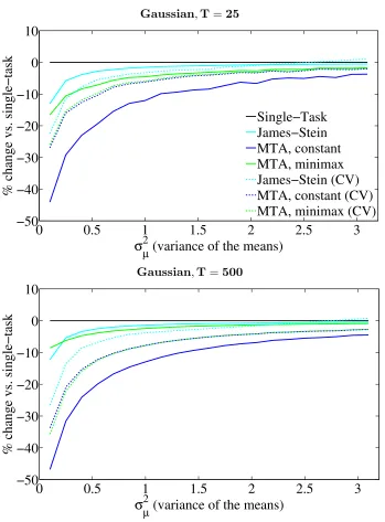
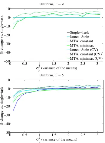
Some observations from Figures 4-7:
• Further to the right on the x-axis the means are more likely to be further apart, and multi-task approaches help less on average compared to the single-task sample means.
• ForT = 2, the James-Stein estimator reduces to the single-task estimator. The MTA estimators provide a gain while the means are close with high probability (that is, when σµ2 <1) but deteriorate quickly thereafter.
• For T = 5, MTA Constant dominates in the Gaussian case, but in the uniform case does worse than single-task when the means are far apart. For all T > 2, MTA Minimax almost always outperforms James-Stein and always outperforms single-task, which is to be expected as it was designed conservatively.
• The T = 25 and T = 500 cases illustrate that all estimators benefit from an increase in the number of tasks. The difference between T = 25 performance and T = 500 performance is minor, indicating that benefit from jointly estimating a larger number of tasks together levels off early on.
• Cross-validating MTA Constant or MTA Minimax should result in similar perfor-mance, and this can be seen in the figures where the green and blue dotted lines are superimposed. The performance differs slightly because the discrete set of γ choices multiply differenta’s for the MTA Constant and MTA Minimax.
In summary, when the tasks are close to each other compared to their variances, MTA Constant is the best estimator to use by a wide margin. When the tasks are farther apart, MTA Minimax provides a win over both James-Stein and sample averages.
5.1 Oracle Performance
To illustrate the best performance we know is possible to achieve with MTA, Figure 8 shows the effect of using the true “oracle” means and variances for the calculation of optimal pairwise similarities for T >2:
Aorclrs = 2
(µr−µs)2
. (22)
This matrix is the best pairwise oracle, but does not generally minimize the risk over all possible A forT >2. However, comparing to it illustrates how well the MTA formulation can do, without the added error due to estimating Afrom the data.3:
Figure 8 reproduces the results from the T = 5 Gaussian simulation (excluding cross-validation results), and compares to the performance of oracle pairwise MTA using (22). Oracle MTA is over 30% better than MTA Constant, indicating that practical estimates of the similarity are highly suboptimal compared to the best possible MTA performance, and motivating better estimates of Aas a direction for future research.
6. Real Data Experiments
We present four real data experiments,4 comparing eight estimators on both goals (2)
and (3). The first experiment estimates future customer reviews based on past customer reviews. The second experiment estimates final grades based on homework grades. The third experiment forecasts a customer’s future order size based on the size of their past orders. The fourth experiment takes a more in-depth look at the estimates produced by these methods for the historical problem of estimating the length of a king’s reign.
6.1 Metrics
For all the experiments except estimating final grades, we only have sample data, and so we compare the estimators using a metric that is an empirical approximation to the regression error defined in (3). First, we replace the expectation in (3) with a sum over the samples. Second, we measure the squared error between a sampleytiand an estimator formed without
3. Preliminary experiments (not reported) showed that forT >2 estimatingApairwise as ˆArs= 2
( ¯yr−¯ys)2
was almost always worse than constant MTA.
4. Research-grade Matlab code and the data used in these experiments can be found athttp://mayagupta.
Gaussian,T=2
0
0.5
1
1.5
2
2.5
3
−50
−40
−30
−20
−10
0
10
σ
µ2
(variance of the means)
% change vs. single−task
Single−Task
James−Stein
MTA, constant
MTA, minimax
James−Stein (CV)
MTA, constant (CV)
MTA, minimax (CV)
Gaussian,T=5
0
0.5
1
1.5
2
2.5
3
−50
−40
−30
−20
−10
0
10
σ
µ 2(variance of the means)
% change vs. single−task
Gaussian,T=25
0
0.5
1
1.5
2
2.5
3
−50
−40
−30
−20
−10
0
10
σ
µ2
(variance of the means)
% change vs. single−task
Single−Task
James−Stein
MTA, constant
MTA, minimax
James−Stein (CV)
MTA, constant (CV)
MTA, minimax (CV)
Gaussian,T=500
0
0.5
1
1.5
2
2.5
3
−50
−40
−30
−20
−10
0
10
σ
µ 2(variance of the means)
% change vs. single−task
Uniform,T=2
0
0.5
1
1.5
2
2.5
3
−50
−40
−30
−20
−10
0
10
σ
µ2
(variance of the means)
% change vs. single−task
Single−Task
James−Stein
MTA, constant
MTA, minimax
James−Stein (CV)
MTA, constant (CV)
MTA, minimax (CV)
Uniform,T=5
0
0.5
1
1.5
2
2.5
3
−50
−40
−30
−20
−10
0
10
σ
µ 2(variance of the means)
% change vs. single−task
Uniform,T=25
0
0.5
1
1.5
2
2.5
3
−50
−40
−30
−20
−10
0
10
σ
µ2
(variance of the means)
% change vs. single−task
Single−Task
James−Stein
MTA, constant
MTA, minimax
James−Stein (CV)
MTA, constant (CV)
MTA, minimax (CV)
Uniform,T=500
0
0.5
1
1.5
2
2.5
3
−50
−40
−30
−20
−10
0
10
σ
µ 2(variance of the means)
% change vs. single−task
0
0.5
1
1.5
2
2.5
3
−80
−60
−40
−20
0
σ
µ2
(variance of the means)
% change vs. single−task
Single−Task
James−Stein
MTA, constant
MTA, minimax
MTA, oracle
Figure 8: Average (over 10000 random draws) percent change in risk vs. single-task with T = 5 for the Gaussian simulation. Oracle MTA uses the true means and variance to specify the weight matrixW.
that sample, ˆyt\yti. That is, the empirical risk we measure is:
T X
t=1
1 Nt
Nt X
i=1
(yti−yˆt\yti) 2
!
. (23)
To make the results more comparable across data sets, we present the results as the percent the error given in (23) is reduced compared to the single-task sample mean estimate.
6.2 Experimental Details
In addition to James-Stein, MTA, and their variants, we also compare to the completely-regularized baseline, the pooled mean estimator:
ˆ
ytpooled= ¯y¯= 1 T N
T X
s=1 N X
i=1
ysi, (24)
which estimates the same value for each task.
For each experiment, a single pooled variance estimate when needed was used for all tasks: σt2 =σ2,for all t. We found that using a pooled variance estimate improved perfor-mance for all the estimators compared.
6.3 Estimating Customer Reviews for Amazon Products
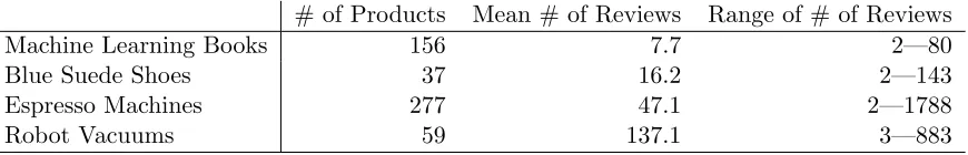
We model amazon.com customer reviews for a product as iid random draws from an un-known distribution. We scraped customer review scores (ranging from 1 to 5) for four different product types from the amazon.com website, as detailed in Table 2. We treat each product as a task, and jointly estimate the mean reviews for all products of the same type. The eight estimators are compared to see how well they predict held-out customer reviews, as per (23); a lower (more negative) score corresponds to greater percent reduction in risk compared to the sample mean estimates.
# of Products Mean # of Reviews Range of # of Reviews
Machine Learning Books 156 7.7 2—80
Blue Suede Shoes 37 16.2 2—143
Espresso Machines 277 47.1 2—1788
Robot Vacuums 59 137.1 3—883
Table 2: Products used in customer reviews experiments, ordered by mean number of re-views (that is, mean sample size).
Table 3 shows the percent risk reduction for each estimator compared to single-task estimates. Some observations:
• MTA Constant (no cross-validation) has the best risk reduction averaged across the products at 11.9% average risk reduction over the single-task estimates, slightly better than the cross-validated forms of MTA.
• The average MTA Constant risk reduction is 34% better than JS (11.9% vs 8.9%), and MTA Constant is better than JS on all the data sets.
• On all data sets, all the joint estimators (not including the pooled mean baseline) do better than the single-task estimates except JS CV on the robot vacuums data set, showing that joint estimation usually helps.
• The JS estimator is more sensitive to the quality of the pooled mean estimate than the MTA Constant estimator.
• JS does better on average than its cross-validated counterpart JS CV, and MTA Constant does better on average than its cross-validated counterpart MTA Constant CV.
• The rows in Table 3 are ordered by the average number of reviews (that is, the average number of samples per task). As one would expect from theory, the gains are larger if there are fewer reviews per task.
• Mixing un-related products (the last row of Table 3) still produces substantial gains over single-task estimates.
Pooled JS JS MTA MTA MTA MTA
Mean CV Constant Constant Minimax Minimax
CV CV
ML Books -24.6 -23.1 -22.9 -24.6 -23.3 -6.5 -23.1
Blue Suede Shoes -12.4 -11.5 -10.6 -12.5 -11.6 -4.8 -11.6
Espresso Machines 2.7 -3.7 -6.3 -8.4 -7.8 -3.6 -8.3
Robot Vacuums 8.7 -0.7 7.3 -2.5 -2.2 -0.8 -1.8
All Products -1.9 -5.4 -9.3 -11.3 -11.0 -4.3 -10.7
Average -5.5 -8.9 -8.4 -11.9 -11.2 -4.0 -11.1
STD 13.2 8.9 10.8 8.1 7.7 2.1 7.7
Table 3: Percent change in risk vs. single-task for customer reviews experiment (lower is better). ‘JS’ denotes James-Stein, ‘CV’ denotes cross-validation, and ‘STD’ denotes standard deviation.
6.4 Estimating Final Grades from Homework Grades
We model homework grades as random samples drawn iid from an unknown distribution where the mean for each student is that student’s final class grade. We compare the eight estimators to see how well they predict each student’s final grade given only their homework grades. Final class grades are based on the homework, but also on projects, labs, quizzes, exams and sometimes class participation, with the mix varying by class. We collected 22 anonymized data sets from six different instructors at three different universities for undergraduate electrical engineering classes. Further experimental details:
• Each of the 22 data sets is for a different class, and constitutes a single experiment, where each student corresponds to a task.
• We treat theith homework grade of the tth student as sample yti.
• For each class, the error measurement for estimator ˆy is the sum of squared errors across allT students:
T X
t=1
(µt−yˆt)2,
whereµt is the giventth student’s final grade.
Table 4 compares the estimators in terms of the percent change in error compared to the single task estimate ¯yt. A lower (more negative) score corresponds to greater percent
reduction in risk compared to the single task estimates. Some observations:
• MTA Constant (no cross-validation) has the best average risk reduction, at 16.6% better on average than the standard single-task estimate. The standard deviation of the win over single task for MTA Constant is 13.7% - also lower than any of the other estimators except MTA Minimax. This shows MTA Constant is consistently providing good error reduction.
• MTA Minimax consistently provides small gains, as designed, with low variance.
• Once again, the higher variance of the James-Stein estimator compared to the others is because of the positive-part aspect of the JS estimator: when the positive-part boundary is triggered, JS reduces to the one-task (average-of-means) estimator, which can have poor performance.
• JS does better on average than its cross-validated counterpart JS CV, and MTA Constant does better on average than its cross-validated counterpart MTA Constant CV.
6.5 Estimating Customer Spending
We collaborated with the wooden jigsaw puzzle company Artifact Puzzles to estimate how much each repeat customer would spend on their next order. We treated each customer as a task; in the time period spanned by the data there are T = 1355 unique customers who have each purchased at least twice. We modelled each order by a customer as an iid draw from that customer’s unknown spending distribution. The number of orders per customer (that is, samples per task) ranged from 2-23, with a mean of 3.03 orders per customer. The amount spent on a given order had a rather long tail distribution, ranging from $9-$2403, with a mean of $82.16.
Results are shown in Table 5, showing the percentage reduction in (23) compared to the single-task sample means.
Some observations from Table 5:
• MTA Constant performed slightly better than the James-Stein estimator, reducing the empirical risk by 22.4% rather than 21.1%.
Class Pooled JS JS MTA MTA MTA MTA
Size Mean CV Constant Constant Minimax Minimax
CV CV
16 26.3 0.7 -0.0 0.6 -0.0 -0.0 -0.0
20 71.2 −3.2 -5.2 −4.7 −3.4 −1.7 −4.6
25 776.9 −12.2 -12.3 −12.2 −12.2 −2.7 −12.1 29 −7.6 −11.6 −31.2 −11.4 -35.2 −1.8 −29.6 34 373.6 −4.9 −12.4 −5.0 −12.7 −1.1 -13.3
36 -28.3 −17.4 −0.0 −16.0 −0.0 −2.8 −0.0
39 42.0 -5.8 −0.0 −5.6 −0.0 −0.9 −0.0
44 3.0 −47.6 −64.5 −42.7 −68.0 −7.0 -69.0
45 127.6 −3.0 −0.0 -19.2 −0.0 −4.6 −0.0 47 -12.8 −8.0 −0.0 −7.1 −0.0 −0.7 −0.0 48 -21.0 −20.5 −0.0 −18.5 −0.0 −2.5 −0.0
50 63.5 63.5 −0.0 9.3 −0.0 -4.4 −0.0
50 3.7 −33.6 −41.5 −29.7 −42.4 −3.2 -47.4
57 23.3 -3.8 −0.0 −3.6 −0.0 −0.4 −0.0
58 −0.2 -16.3 −0.0 −15.6 −0.0 −2.8 −0.0 65 45.0 -29.4 −0.0 −26.2 −0.0 −4.2 −0.0 68 −16.9 -45.5 −16.5 −39.0 −17.0 −6.1 −19.8 69 −14.7 -41.0 −14.7 −39.8 −14.7 −4.5 −14.8 72 34.6 −32.9 −27.3 −29.0 −27.8 −4.0 -34.8
73 224.2 −28.1 −41.1 −26.4 −39.6 −2.4 -41.2
110 5.7 −14.8 -25.3 −13.4 −20.6 −1.2 −22.0 149 -16.6 −11.7 −0.0 −10.1 −0.0 −0.8 −0.0 Average 77.4 −14.9 −13.3 -16.6 −13.3 −2.7 −14.0
STD 182.0 22.7 18.1 13.7 18.7 1.9 19.4
Pooled JS JS MTA MTA MTA MTA
Mean CV Constant Constant Minimax Minimax
CV CV
Customer Spending -10.6 -21.1 -17.6 -22.4 -19.7 -0.6 -19.5
Table 5: Percent change in risk vs. single-task for the customer spending experiments (lower is better). ‘JS’ denotes James-Stein, ‘CV’ denotes cross-validation.
Pooled JS JS MTA MTA MTA MTA
Mean CV Constant Constant Minimax Minimax
CV CV
Kings’ Reigns -8.2 -8.7 -4.7 -8.9 -2.9 -3.1 -3.2
Table 6: Percent change in risk vs. single-task for the kings’ reigns experiments (lower is better). ‘JS’ denotes James-Stein, ‘CV’ denotes cross-validation.
6.6 Estimating the Length of Kings’ Reigns
To illustrate the differences between the actual estimates, we re-visit an estimation problem studied by Isaac Newton, “How long does the average king reign?” (Newton, 1728; Stigler, 1999). Newton considered 9 different kingdoms, from the Kings of Judah to more recent French kings. Our data set covers 30 well-known dynasties, listed in Table 7, from ancient to modern times, and spread across the globe. All data was taken from wikipedia.org in August and September 2013 (see the linked data files for the raw data and more historical details).
Results are shown in Table 6, showing the percentage reduction in (23) compared to the single-task sample means. Some observations about these results:
• The pooled mean is 8.2% better than estimating each dynasty’s average separately. We found it surprising that pooling across cultures and history forms overall better estimates: the fate of man is apparently the fate of man, regardless of whether it is 1000 BC in Babylon or 19th century Denmark.
• The JS and MTA Constant estimators achieve a slightly bigger reduction in squared error compared to the pooled mean.
• The MTA Constant estimator is very slightly better than the JS estimator,−8.9% vs
−8.7%.
• The JS and MTA estimators do better than their cross-validated counterparts.
Dynasty, # Kings Avg. Pooled JS JS MTA MTA MTA MTA
Mean CV Const. Const. MM MM
CV CV
Larsa, 15 17.7 19.5 19.2 18.5 18.3 18.1 17.8 18.1 Amorite, 11 26.9 19.5 22.3 24.6 24.6 25.5 26.5 25.6 Assyrian, 27 17.3 19.5 19.1 18.2 17.8 17.6 17.4 17.6 Israel, 21 13.4 19.5 17.7 15.6 14.8 14.2 13.6 14.1 Judah, 22 21.5 19.5 20.5 21.0 21.2 21.3 21.5 21.4 Achaemenid, 9 24.3 19.5 21.4 22.9 22.4 23.1 23.9 23.2 Khmer, 33 20.0 19.5 20.0 20.0 20.0 20.0 20.0 20.0 Song, 18 17.7 19.5 19.2 18.5 18.3 18.0 17.8 18.0 Mongol, 4 10.8 19.5 16.8 13.8 16.1 14.5 12.0 14.3 Ming, 17 16.3 19.5 18.7 17.5 17.2 16.8 16.4 16.8 Qing, 12 24.6 19.5 21.6 23.0 23.1 23.7 24.4 23.8 Mamluk, 10 10.1 19.5 16.6 13.4 13.6 12.3 10.7 12.1 Ottoman, 36 17.0 19.5 19.0 18.0 17.4 17.2 17.1 17.2 Normandy, 3 23.0 19.5 21.0 22.0 21.1 21.6 22.5 21.7 Plantagenet, 8 30.8 19.5 23.7 27.2 26.4 28.0 30.0 28.2 Lancaster, 3 20.3 19.5 20.1 20.2 20.1 20.2 20.3 20.2
York, 3 8.0 19.5 15.9 12.0 15.8 13.8 10.1 13.4
Tudor, 5 23.4 19.5 21.1 22.3 21.6 22.2 23.0 22.3 Stuart, 6 16.8 19.5 18.9 17.9 18.4 17.8 17.1 17.8 Hanover, 6 31.0 19.5 23.7 27.3 25.7 27.5 30.0 27.8 Windsor, 3 14.0 19.5 17.9 16.0 17.9 16.9 15.0 16.7 Capet, 15 22.7 19.5 20.9 21.8 21.9 22.3 22.6 22.3 Valois, 7 24.3 19.5 21.4 22.9 22.4 23.1 23.9 23.2 Habsburg, 5 34.4 19.5 24.9 29.6 26.8 29.3 32.8 29.6 Bourbon, 10 21.8 19.5 20.6 21.2 21.2 21.4 21.7 21.4 Oldenburg, 16 25.8 19.5 22.0 23.9 24.3 25.0 25.6 25.0 Mughal, 20 15.7 19.5 18.5 17.1 16.6 16.2 15.8 16.2 Edo, 15 18.6 19.5 19.5 19.1 19.0 18.8 18.7 18.8 Kamehameha, 5 15.4 19.5 18.4 16.9 17.8 17.1 15.9 16.9 Zulu, 4 15.8 19.5 18.5 17.2 18.2 17.5 16.3 17.4 Average
Over Dynasties 19.98 19.49 19.98 19.98 20.00 20.03 20.01 20.04
• Table 7 shows that while all the estimators regularize the single task mean (given in column 1) to the pooled mean (given in column 2), the actual estimates can differ quite a bit. For example, MTA Constant and MTA Minimax differ by 5 years in their estimates of the average length of reign of a king from the House of York.
• One sees that the JS estimates are regularized harder towards the pooled mean of 19.5 than the MTA Constant estimates. The MTA Minimax estimates are (as expected) least changed from the task means.
• The last row of Table 7 shows the estimates averaged over the different dynasties. Note that the JS and JS CV estimators have the same average across the tasks (dynasties) as the single-task average, as expected from Proposition 7.
• Based on Tables 5 and 7, we estimate the expected length of a king’s reign to be the dynasty-averaged MTA Constant estimate of 20.00 years. Newton’s wrote his estimate as “eighteen or twenty years” (Newton, 1728), and the analysis of Stigler (1999) of Newton’s data shows that the maximum likelihood estimate from his data was a more pessimistic 19.03 years.
7. Conclusions And Open Questions
We conclude with a summary and then some open questions.
7.1 Summary
We proposed a simple additive regularizer to jointly estimate multiple means using a pair-wise task similarity matrix A. Our analysis of the T = 2 task case establishes that both MTA estimates are better than the individual sample means when the separation between the true means is small relative to the variance of the samples from each distribution. For the two-task case, we provide a formula for the optimal pairwise task similarity matrix A, that is, one can analytically estimate the optimal amount of regularization without the need to cross-validate or tune a regularization hyper-parameter. We generalized that for-mula to multiple tasks to form the practical and computationally-efficient MTA Constant mean estimator, as well as a more conservative minimax variant. Simulations and four sets of real data experiments show the MTA Constant estimator can substantially reduce errors over the sample means, and generally performs slightly better than James-Stein estimation (which also does not require cross-validation).
One can also cross-validate the amount of regularization in the MTA formula or in the James-Stein formula. Our results show that both cross-validations work well, though in both simulations and real data experiments, MTA Constant performed slightly better or comparable to the cross-validations.
7.2 Open Questions
Most multi-task learning formulations contain an explicit or implicit dependence on the pairwise similarity between tasks. For MTA, this is the A matrix. Even when side information about task similarities is available, it may not be in the optimal numerical form. This paper shows good performance with the assumption thatAhas constant entries, where that constant is the average of pairwise similarities estimated based on the sample means (MTA Constant). However, the oracle performance plots in Section 5 show that the right choice ofAcan perform much better. Estimating allT×T parameters ofAoptimally may be difficult, but we hypothesize that other structured assumptions, such as low rankA, might perform better than our constant approximation. Mart´ınez-Rego and Pontil (2013) have shown some promising results by clustering tasks in a pre-processing stage.
We focused in this paper on estimating scalar means. The extension to vectors is straightforward (see Section 4.2). However, how well the vector extension works in prac-tice, how to best estimate the block diagonal covariance matrix, and whether different regularization norms would be better remain open questions. A further extension is when the samples themselves are distributions, and the task means to be estimated are expected distributions (Frigyik et al., 2008).
We showed in Section 4 that the matrix inverse needed to compute the MTA Constant and MTA Minimax estimators can be done efficiently. Simulations showed that the achiev-able gains generally go up slowly with the number of tasks T, with T = 500 producing an average risk reduction of 40% in the extreme case that the true means for the 500 tasks were the same. In the real data experiment on customer spending, there were T = 1355 tasks that produced a risk reduction of 22.4%. Larger-scale experiments and analysis of the effect of large T on the error would be intriguing.
We focused on squared error loss and the graph Laplacian regularizer because they are standard, generally work well, lead to computationally efficient solutions, and are easy to analyze. But re-considering the MTA objective with other loss functions and regularizers might lead to interesting new perspectives and estimates.
Lastly, we hope that some of the analyses and results in this paper inspire further theoretical analysis of other multi-task learning methods.
Acknowledgments
This work was funded by a United States PECASE Award and by the United States Office of Naval Research. We thank Peter Sadowski for helpful discussions.
Appendix A. MTA Closed-form Solution
When all Ars are non-negative, the differentiable MTA objective is convex, and admits
L=D−(A+A>)/2: 1 T T X t=1 1 σ2 t Nt X i=1
(Yti−Y˜t)2+
γ T2 T X r=1 T X s=1
Ars( ˜Yr−Y˜s)2
= 1 T T X t=1 1 σt2
Nt X
i=1
Yti2+ Nt σ2t ˜
Yt2−2Nt σt2
˜ YtY¯t
!
+ γ T2Y˜
>LY˜
= 1 T T X t=1 1 σ2 t Nt X i=1
Yti2+ ˜Y>Σ−1Y˜ −2 ˜Y>Σ−1Y¯
!
+ γ T2Y˜
>
LY ,˜
where, Σ is a diagonal matrix with Σtt = σ 2 t
Nt, and ˜Y and ¯Y are column vectors with tth
entries ˜Yt and ¯Yt, respectively.
For simplicity of notation, we assume from now on that Ais symmetric. If, in practice, an asymmetric Ais provided, it can be symmetrized without loss of generality.
Take the partial derivative of the above objective w.r.t. ˜Y and equate to zero,
0 = 1
T 2Σ
−1Y∗−2Σ−1Y¯
+ 2 γ
T2LY
∗ (25)
=Y∗−Y¯ + γ
TΣLY
∗
¯
Y =I+ γ
TΣL
Y∗,
which yields the following optimal closed-form solution:
Y∗ =
I+ γ
TΣL
−1
¯
Y , (26)
as long as the inverse exists, which we will prove next.
Appendix B. Proof of Lemma 1
Assumptions: γ ≥0, 0≤Ars<∞for all r, s and 0< σ 2 t
Nt <∞ for allt.
Lemma 1 The MTA solution matrix W = I+TγΣL−1 exists.
Proof Let B =W−1 =I+ TγΣL. The (t, s)th entry of B is
Bts =
(
1 + γσt2 T Nt
P
s6=tAts ift=s −γσ2t
T NtAts ift6=s,
The Gershgorin disk (Horn and Johnson, 1990)D(Btt, Rt) is the closed disk inCwith center
Btt and radius
Rt=
X
s6=t
|Bts|=
γσt2 T Nt
X
s6=t
One knows that Btt ≥ 1 for non-negative A and when γσ 2 t
T Nt ≥ 0, as assumed prior to the
lemma statement. Also, it is clear thatBtt> Rtfor all t. Therefore, every Gershgorin disk
is contained within the positive half-plane of C, and, by the Gershgorin Circle Theorem
(Horn and Johnson, 1990), the real part of every eigenvalue of matrix B is positive. Its determinant is therefore positive, and the matrix B is invertible: W =B−1.
Appendix C. Proof of Proposition 2
Recall the proposition: As Nt→ ∞∀ t, Y∗→µ.
Proof First note that the (t, t)th diagonal entry of Σ is σt2
Nt, which approaches 0 asNt→0,
implying that all entries of TγΣL → 0 as Nt → 0 as well. Since matrix inversion is a
continuous operation, I+ TγΣL−1 → I in the norm.5 By the law of large numbers one can conclude that Y∗ asymptotically approaches the true mean µ.
Note further that the above proof is only valid for diagonal Σ, but can be easily ex-tended for non-diagonal Σ by noting that Σrs= √σNrσs
rNs also converges to 0 asNr, Ns→0.
Appendix D. Proof of Theorem 3
Assumptions: γ ≥0, 0≤Ars<∞for all r, s and 0< σ 2 t
Nt <∞ for allt.
We next state and prove two lemmas that will be used to prove Theorem 3.
Lemma 8 W has all non-negative entries.
Proof Because the off-diagonal elements of the graph Laplacian are non-positive, W−1= I+TγΣL
is a Z-matrix, defined to be a matrix with non-positive off-diagonal entries (Berman and Plemmons, 1979). If W−1 is a Z-matrix, then the following two statements are true and equivalent: “the real part of each eigenvalue ofW−1 is positive” and “W exists and W ≥ 0 (elementwise)” (Berman and Plemmons, 1979, Chapter 6, Theorem 2.3, G20
and N38). It has already been proven in Lemma 1 that the real part of every eigenvalue of
W−1 is positive. Therefore,W exists and is element-wise non-negative.
Lemma 9 The rows of W sum to 1.
Proof As proved in Lemma 1, W exists. Therefore, one can write:
W1=1
1=W−11
=I+ γ
TΣL
1
=I1+ γ
TΣL1
=1+ γ
TΣ0
=1,
where the the third equality is true because the graph Laplacian has rows that sum to zero. The rows ofW therefore sum to 1.
Theorem 3 The MTA solution matrix W = I+TγΣL−1
is right-stochastic.
Proof We know thatW exists (from Lemma 1), is entry-wise non-negative (from Lemma 8), and has rows that sum to 1 (from Lemma 9).
Appendix E. MTA Constant Derivation
For the case whenT >2, analytically specifying a general similarity matrixAthat minimizes the risk is intractable. To address this limitation for arbitraryT, we constrain the similarity matrix to be the constant matrix A=a11>, resulting in the following weight matrix:
Wcnst=
I+ 1
TΣL(a11
> )
−1
. (27)
For tractability, we optimize ausingtr(Σ)I rather than the full Σ matrix, such that
a∗ = arg min
a
R µ,
I+ 1
T
tr(Σ)
T L(a11
> )
−1
¯ Y
!
, (28)