A Theory of Multiclass Boosting
Indraneel Mukherjee IMUKHERJ@CS.PRINCETON.EDU
1600 Amphitheatre Parkway Mountain View, CA 94043, USA
Robert E. Schapire SCHAPIRE@CS.PRINCETON.EDU
Princeton University
Department of Computer Science Princeton, NJ 08540 USA
Editor:Manfred Warmuth
Abstract
Boosting combines weak classifiers to form highly accurate predictors. Although the case of binary classification is well understood, in the multiclass setting, the “correct” requirements on the weak classifier, or the notion of the most efficient boosting algorithms are missing. In this paper, we create a broad and general framework, within which we make precise and identify the optimal requirements on the weak-classifier, as well as design the most effective, in a certain sense, boosting algorithms that assume such requirements.
Keywords: multiclass, boosting, weak learning condition, drifting games
1. Introduction
Boosting (Schapire and Freund, 2012) refers to a general technique of combining rules of thumb, or weak classifiers, to form highly accurate combined classifiers. Minimal demands are placed on the weak classifiers, so that a variety of learning algorithms, also called weak-learners, can be employed to discover these simple rules, making the algorithm widely applicable. The theory of boosting is well-developed for the case of binary classification. In particular, the exact requirements on the weak classifiers in this setting are known: any algorithm that predicts better than random on any distribution over the training set is said to satisfy the weak learning assumption. Further, boosting algorithms that minimize loss as efficiently as possible have been designed. Specifically, it is known that the Boost-by-majority (Freund, 1995) algorithm is optimal in a certain sense, and that AdaBoost (Freund and Schapire, 1997) is a practical approximation.
Such an understanding would be desirable in the multiclass setting as well, since many natural classification problems involve more than two labels, for example, recognizing a digit from its image, natural language processing tasks such as part-of-speech tagging, and object recognition in vision. However, for such multiclass problems, a complete theoretical understanding of boosting is lacking. In particular, we do not know the “correct” way to define the requirements on the weak classifiers, nor has the notion of optimal boosting been explored in the multiclass setting.
requiring more than 50% accuracy even when the number of labels is much larger than two is too stringent, and simple weak classifiers like decision stumps fail to meet this criterion, even though they often can be combined to produce highly accurate classifiers (Freund and Schapire, 1996a). The most common approaches so far have relied on reductions to binary classification (Allwein et al., 2000), but it is hardly clear that the weak-learning conditions implicitly assumed by such reductions are the most appropriate.
The purpose of a weak-learning condition is to clarify the goal of the weak-learner, thus aiding in its design, while providing a specific minimal guarantee on performance that can be exploited by a boosting algorithm. These considerations may significantly impact learning and generalization be-cause knowing the correct weak-learning conditions might allow the use of simpler weak classifiers, which in turn can help prevent overfitting. Furthermore, boosting algorithms that more efficiently and effectively minimize training error may prevent underfitting, which can also be important.
In this paper, we create a broad and general framework for studying multiclass boosting that formalizes the interaction between the boosting algorithm and the weak-learner. Unlike much, but not all, of the previous work on multiclass boosting, we focus specifically on the most natural, and perhaps weakest, case in which the weak classifiers are genuine classifiers in the sense of predicting a single multiclass label for each instance. Our new framework allows us to express a range of weak-learning conditions, both new ones and most of the ones that had previously been assumed (often only implicitly). Within this formalism, we can also now finally make precise what is meant bycorrectweak-learning conditions that are neither too weak nor too strong.
We focus particularly on a family of novel weak-learning conditions that have an especially appealing form: like the binary conditions, they require performance that is only slightly better than random guessing, though with respect to performance measures that are more general than ordinary classification error. We introduce a whole family of such conditions since there are many ways of randomly guessing on more than two labels, a key difference between the binary and multiclass settings. Although these conditions impose seemingly mild demands on the weak-learner, we show that each one of them is powerful enough to guarantee boostability, meaning that some combination of the weak classifiers has high accuracy. And while no individual member of the family is necessary for boostability, we also show that the entire family taken together is necessary in the sense that for every boostable learning problem, there exists one member of the family that is satisfied. Thus, we have identified a family of conditions which, as a whole, is necessary and sufficient for multiclass boosting. Moreover, we can combine the entire family into a single weak-learning condition that is necessary and sufficient by taking a kind of union, or logicalOR, of all the members. This combined condition can also be expressed in our framework.
Employing proper weak-learning conditions is important, but we also need boosting algorithms that can exploit these conditions to effectively drive down error. For a given weak-learning condi-tion, the boosting algorithm that drives down training error most efficiently in our framework can be understood as the optimal strategy for playing a certain two-player game. These games are non-trivial to analyze. However, using the powerful machinery of drifting games (Freund and Opper, 2002; Schapire, 2001), we are able to compute the optimal strategy for the games arising out of each weak-learning condition in the family described above. Compared to earlier work, our optimality results hold more generally and also achieve tighter bounds. These optimal strategies have a natu-ral interpretation in terms of random walks, a phenomenon that has been observed in other settings (Abernethy et al., 2008; Freund, 1995).
We also analyze the optimal boosting strategy when using the minimal weak learning condition, and this poses additional challenges. Firstly, the minimal weak learning condition has multiple nat-ural formulations—for example, as the union of all the conditions in the family described above, or the formulation used in AdaBoost.MR—and each formulation leading to a different game specifica-tion. A priori, it is not clear which game would lead to the best strategy. We resolve this dilemma by proving that the optimal strategies arising out of different formulations of the same weak learning condition lead to algorithms that are essentially equally good, and therefore we are free to choose whichever formulation leads to an easier analysis without fear of suffering in performance. We choose the union of conditions formulation, since it leads to strategies that share the same inter-pretation in terms of random walks as before. However, even with this choice, the resulting games are hard to analyze, and although we can explicitly compute the optimum strategies in general, the computational complexity is usually exponential in the number of classes. Nevertheless, we identify key situations under which efficient computation is possible.
The game-theoretic strategies are non-adaptive in that they presume prior knowledge about the
edge, that is, how much better than random are the weak classifiers. Algorithms that are adaptive, such as AdaBoost, are much more practical because they do not require such prior information. We show therefore how to derive an adaptive boosting algorithm by modifying the game-theoretic strategy based on the minimal condition. This algorithm enjoys a number of theoretical guarantees. Unlike some of the non-adaptive strategies, it is efficiently computable, and since it is based on the minimal weak learning condition, it makes minimal assumptions. In fact, whenever presented with a boostable learning problem, this algorithm can approach zero training error at an exponential rate. More importantly, the algorithm is effective even beyond the boostability framework. In particular, we show empirical consistency, that is, the algorithm always converges to the minimum of a certain exponential loss over the training data, whether or not the data set is boostable. Furthermore, using the results in Mukherjee et al. (2011) we can show that this convergence occurs rapidly.
under certain conditions and with sufficient data, our adaptive algorithm approaches the Bayes-optimum error on thetestdata set.
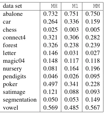
We present experiments aimed at testing the efficacy of the adaptive algorithm when working with a very weak weak-learner to check that the conditions we have identified are indeed weaker than others that had previously been used. We find that our new adaptive strategy achieves low test error compared to other multiclass boosting algorithms which usually heavily underfit. This validates the potential practical benefit of a better theoretical understanding of multiclass boosting.
1.1 Previous Work
The first boosting algorithms were given by Schapire (1990) and Freund (1995), followed by their AdaBoost algorithm (Freund and Schapire, 1997). Multiclass boosting techniques include Boost.M1 and AdaBoost.M2 (Freund and Schapire, 1997), as well as AdaBoost.MH and Ada-Boost.MR (Schapire and Singer, 1999). Other approaches include the work by Eibl and Pfeiffer (2005) and Zhu et al. (2009). There are also more general approaches that can be applied to boosting including Allwein et al. (2000), Beygelzimer et al. (2009), Dietterich and Bakiri (1995), Hastie and Tibshirani (1998) and Li (2010). Two game-theoretic perspectives have been applied to boosting. The first one (Freund and Schapire, 1996b; R¨atsch and Warmuth, 2005) views the weak-learning condition as a minimax game, while drifting games (Schapire, 2001; Freund, 1995) were designed to analyze the most efficient boosting algorithms. These games have been further analyzed in the multiclass and continuous time setting in Freund and Opper (2002).
2. Framework
We introduce some notation. Unless otherwise stated, matrices will be denoted by bold capital letters like M, and vectors by bold small letters like v. Entries of a matrix and vector will be denoted asM(i,j)orv(i), whileM(i)will denote theith row of a matrix. The inner product of two vectorsu,vis denoted byhu,vi. The Frobenius inner product Tr(AB′)of two matricesA,Bwill be denoted byA•B′, whereB′is the transpose ofB. The indicator function is denoted by1[·]. The set of all distributions over the set{1, . . . ,k}will be denoted by∆{1, . . . ,k}, and in general, the set of all distributions over any setSwill be denoted by∆(S).
In multiclass classification, we want to predict the labels of examples lying in some setX. We are provided a training set of labeled examples{(x1,y1), . . . ,(xm,ym)}, where each examplexi∈X has a labelyi in the set{1, . . . ,k}.
Boosting combines several mildly powerful predictors, calledweak classifiers, to form a highly accurate combined classifier, and has been previously applied for multiclass classification. In this paper, we only allow weak classifiers that predict a single class for each example. This is appealing, since the combined classifier has the same form, although it differs from what has been used in much previous work. Later we will expand our framework to includemultilabel weak classifiers, that may predict multiple labels per example.
• Booster creates a cost-matrixCt ∈Rm×k, specifying to Weak-Learner that the cost of classi-fying examplexiaslisCt(i,l). The cost-matrix may not be arbitrary, but should conform to certain restrictions as discussed below.
• Weak-Learner returns some weak classifierht:X→ {1, . . . ,k}from a fixed spaceht∈
H
so that the cost incurred isCt•1ht = m
∑
i=1Ct(i,ht(xi)),
is “small enough”, according to some conditions discussed below. Here by1h we mean the
m×kmatrix whose(i,j)-th entry is1[h(i) = j].
• Booster computes a weightαt for the current weak classifier based on how much cost was incurred in this round.
At the end, Booster predicts according to the weighted plurality vote of the classifiers returned in each round:
H(x)=△ argmax l∈{1,...,k}
fT(x,l), where fT(x,l)
△
= T
∑
t=11[ht(x) =l]αt. (1)
By carefully choosing the cost matrices in each round, Booster aims to minimize the training error of the final classifierH, even when Weak-Learner is adversarial. The restrictions on cost-matrices created by Booster, and the maximum cost Weak-Learner can suffer in each round, together define theweak-learning conditionbeing used. For binary labels, the traditional weak-learning condition states: for any non-negative weightsw(1), . . . ,w(m)on the training set, the error of the weak classi-fier returned is at most(1/2−γ/2)∑iwi. Hereγparametrizes the condition. There are many ways to translate this condition into our language. The one with fewest restrictions on the cost-matrices requires labeling correctly should be less costly than labeling incorrectly:
∀i:C(i,yi)≤C(i,y¯i)(here ¯yi6=yiis the other binary label),
while the restriction on the returned weak classifierhrequires less cost than predicting randomly:
∑
iC(i,h(xi))≤
∑
i
1 2−
γ
2
C(i,y¯i) +
1 2+
γ
2
C(i,yi)
.
By the correspondencew(i) =C(i,y¯i)−C(i,yi), we may verify the two conditions are the same. We will rewrite this condition after making some simplifying assumptions. Henceforth, without loss of generality, we assume that the true label is always 1. Let
C
bin ⊆Rm×2 consist of matri-ces Cwhich satisfyC(i,1)≤C(i,2). Further, let Ubinγ ∈Rm×2 be the matrix whose each row is (1/2+γ/2,1/2−γ/2). Then, Weak-Learner searching spaceH
satisfies the binary weak-learning condition if: ∀C∈C
bin,∃h∈H
:C• 1h−Ubinγ
Let
C
⊆Rm×kand letB∈Rm×kbe a matrix which we call thebaseline. We say a weak classifier spaceH
satisfies the condition(C
,B)if∀C∈
C
,∃h∈H
: C•(1h−B)≤0, i.e., m∑
i=1C(i,h(i))≤ m
∑
i=1hC(i),B(i)i. (2)
In (2), the variable matrix Cspecifies how costly each misclassification is, while the baseline B specifies a weight for each misclassification. The condition therefore states that a weak classi-fier should not exceed the average cost when weighted according to baseline B. This large class of weak-learning conditions captures many previously used conditions, such as the ones used by AdaBoost.M1 (Freund and Schapire, 1996a), AdaBoost.MH (Schapire and Singer, 1999) and Ada-Boost.MR (Freund and Schapire, 1996a; Schapire and Singer, 1999) (see below), as well as novel conditions introduced in the next section.
By studying this vast class of weak-learning conditions, we hope to find the one that will serve the main purpose of the boosting game: finding a convex combination of weak classifiers that has zero training error. For this to be possible, at the minimum the weak classifiers should be sufficiently rich for such a perfect combination to exist. Formally, a collection
H
of weak classifiers isboostableif it is eligible for boosting in the sense that there exists a weighting λ on the votes forming a
distribution that linearly separates the data: ∀i: argmaxl∈{1,...,k}∑h∈Hλ(h)1[h(xi) =l] =yi. The weak-learning condition plays two roles. It rejects spaces that are not boostable, and provides an algorithmic means of searching for the right combination. Ideally, the second factor will not cause the weak-learning condition to impose additional restrictions on the weak classifiers; in that case, the weak-learning condition is merely a reformulation of being boostable that is more appropriate for deriving an algorithm. In general, it could betoo strong, that is, certain boostable spaces will fail to satisfy the conditions. Or it could betoo weak, that is, non-boostable spaces might satisfy such a condition. Booster strategies relying on either of these conditions will fail to drive down error, the former due to underfitting, and the latter due to overfitting. Later we will describe conditions captured by our framework that avoid being too weak or too strong. But before that, we show in the next section how our flexible framework captures weak learning conditions that have appeared previously in the literature.
3. Old Conditions
In this section, we rewrite, in the language of our framework, the weak learning conditions ex-plicitly or imex-plicitly employed in the multiclass boosting algorithms SAMME (Zhu et al., 2009), AdaBoost.M1 (Freund and Schapire, 1996a), and AdaBoost.MH and AdaBoost.MR (Schapire and Singer, 1999). This will be useful later on for comparing the strengths and weaknesses of the var-ious conditions. We will end this section with a curvar-ious equivalence between the conditions of AdaBoost.MH and AdaBoost.M1.
Recall that we have assumed the correct label is 1 for every example. Nevertheless, we continue to useyito denote the correct label in this section.
3.1 Old Conditions in the New Framework
3.1.1 SAMME
The SAMME algorithm (Zhu et al., 2009) requires less error than random guessing on any distribu-tion on the examples. Formally, a space
H
satisfies the condition if there is aγ′>0 such that,∀d(1), . . . ,d(m)≥0,∃h∈
H
: m∑
i=1d(i)1[h(xi)6=yi]≤(1−1/k−γ′) m
∑
i=1d(i). (3)
Define a cost matrixCwhose entries are given by
C(i,j) =
(
d(i) if j6=yi, 0 if j=yi.
Then the left hand side of (3) can be written as m
∑
i=1C(i,h(xi)) =C•1h.
Next letγ= (k/(k−1))γ′and define baselineU
γto be the multiclass extension ofUbin, Uγ(i,l) =
((1
−γ)
k +γ ifl=yi,
(1−γ)
k ifl6=yi. Then notice that for eachi, we have
C(i),Uγ(i) =
∑
l6=yiC(i,l)Uγ(i,l)
= (k−1)(1−γ)
k d(i)
=
1−1
k−
1−1
k
γ
d(i)
=
1−1
k−γ ′
d(i).
Therefore, the right hand side of (3) can be written as m
∑
i=1l∑
6=yiC(i,l)Uγ(i,l) =C•Uγ,
sinceC(i,yi) =0 for every examplei. Define
C
SAMto be the following collection of cost matrices:C
SAM=△(
C:C(i,l) =
(
0 ifl=yi,
ti ifl6=yi,
for non-negativet1, . . . ,tm.
)
Using the last two equations, (3) is equivalent to
∀C∈
C
SAM,∃h∈H
:C• 1 h−Uγ
≤0.
3.1.2 ADABOOST.M1
AdaBoost.M1 (Freund and Schapire, 1997) measures the performance of weak classifiers using or-dinary error. It requires 1/2+γ/2 accuracy with respect to any non-negative weightsd(1), . . . ,d(m) on the training set:
m
∑
i=1d(i)1[h(xi)=6 yi] ≤ (1/2−γ/2) m
∑
i=1d(i), (4)
i.e., m
∑
i=1d(i)Jh(xi)6=yiK ≤ −γ m
∑
i=1d(i).
whereJ·Kis the ±1 indicator function, taking value+1 when its argument is true, and−1 when false. Using the transformation
C(i,l) =Jl6=yiKd(i)
we may rewrite (4) as
∀C∈Rm×k satisfying 0≤ −C(i,y
i) =C(i,l)forl6=yi, (5) ∃h∈
H
:m
∑
i=1C(i,h(xi))≤γ m
∑
i=1C(i,yi)
i.e., ∀C∈
C
M1,∃h∈H
:C• 1h−BM1γ
≤0,
whereBM1γ (i,l) =γ1[l=yi], and
C
M1⊆Rm×kconsists of matrices satisfying the constraints in (5). 3.1.3 ADABOOST.MHAdaBoost.MH (Schapire and Singer, 1999) is a popular multiclass boosting algorithm that is based on the one-against-all reduction, and was originally designed to use weak-hypotheses that return a prediction for every example and every label. The implicit weak learning condition requires that for any matrix with non-negative entriesd(i,l), the weak-hypothesis should achieve 1/2+γaccuracy
m
∑
i=1(
1[h(xi)6=yi]d(i,yi) +
∑
l6=yi1[h(xi) =l]d(i,l)
) ≤ 1 2− γ 2 m
∑
i=1k
∑
l=1d(i,l).
(6)
This can be rewritten as
m
∑
i=1(
−1[h(xi) =yi]d(i,yi) +
∑
l6=yi1[h(xi) =l]d(i,l)
)
≤ m
∑
i=1( 1 2− γ 2
∑
l6=yid(i,l)−
1 2+ γ 2
d(i,yi)
)
.
Using the mapping
C(i,l) =
(
their weak-learning condition may be rewritten as follows
∀C∈Rm×ksatisfyingC(i,y
i)≤0,C(i,l)≥0 forl6=yi, (7) ∃h∈
H
:summi=1C(i,h(xi))≤ m
∑
i=1( 1 2+ γ 2
C(i,yi) +
1 2− γ 2
∑
l6=yiC(i,l)
)
.
Defining
C
MHto be the space of all cost matrices satisfying the constraints in (7), the above condi-tion is the same as∀C∈
C
MH,∃h∈H
:C• 1h−BMHγ
≤0,
whereBMH
γ (i,l) = (1/2+γJl=yiK/2).
3.1.4 ADABOOST.MR
AdaBoost.MR (Schapire and Singer, 1999) is based on the all-pairs multiclass to binary reduction. Like AdaBoost.MH, it was originally designed to use weak-hypotheses that return a prediction for every example and every label. The weak learning condition for AdaBoost.MR requires that for any non-negative cost-vectors{d(i,l)}l6=yi, the weak-hypothesis returned should satisfy the following:
m
∑
i=1l∑
6=yi(1[h(xi) =l]−1[h(xi) =yi])d(i,l) ≤ −γ m
∑
i=1l∑
6=yid(i,l)
i.e., m
∑
i=1(
−1[h(xi) =yi]
∑
l6=yid(i,l) +
∑
l6=yi1[h(xi) =l]d(i,l)
)
≤ −γ
m
∑
i=1l∑
6=yid(i,l).
Substituting
C(i,l) =
(
d(i,l) l6=yi −∑l6=yid(i,l) l=yi, we may rewrite AdaBoost.MR’s weak-learning condition as
∀C∈Rm×ksatisfyingC(i,l)
≥0 forl6=yi,C(i,yi) =−
∑
l6=yiC(i,l), (8)
∃h∈
H
: m∑
i=1C(i,h(xi))≤ −
γ
2 m
∑
i=1(
−C(i,yi) +
∑
l6=yiC(i,l)
)
.
Defining
C
MRto be the collection of cost matrices satisfying the constraints in (8), the above con-dition is the same as∀C∈
C
MR,∃h∈H
:C• 1h−BMRγ
≤0,
whereBMR
γ (i,l) =Jl=yiKγ/2.
3.2 A Curious Equivalence
whereas AdaBoost.MH is based on the one-against-all multiclass to binary reduction. This equiva-lence is a sort of degeneracy, and arises because the weak classifiers being used predict single labels per example. With multilabel weak classifiers, for which AdaBoost.MH was originally designed, the equivalence no longer holds.
The proofs in this and later sections will make use of the following minimax result, that is a weaker version of Corollary 37.3.2 of Rockafellar (1970).
Theorem 1 (Minimax Theorem) Let C,D be non-empty closed convex subsets of Rm,Rn
respec-tively, and let K be a linear function on C×D. If either C or D is bounded, then
min
v∈Dmaxu∈CK(u,v) =maxu∈C minv∈DK(u,v). Lemma 2 A weak classifier space
H
satisfies(C
M1,BM1γ )if and only if it satisfies(
C
MH,BMHγ ). Note thatC
M1andC
MHdepend implicitly on the training set. This lemma is valid for all training sets.Proof We will refer to(
C
M1,BM1γ )by M1 and(
C
MH,BMHγ )by MH for brevity. The proof is in three steps.Step (i): If
H
satisfies MH, then it also satisfies M1. This follows since any constraint (4) imposed by M1 onH
can be reproduced by MH by plugging the following values ofd(i,l)in (6)d(i,l) =
(
d(i) ifl=yi 0 ifl6=yi.
Step (ii): If
H
satisfies M1, then there is a convex combinationHλ∗ of the matrices1h∈H
,defined as
Hλ∗
△
=
∑
h∈Hλ∗(h)1h,
such that
∀i: Hλ∗−BM1γ (i,l)
(
≥0 ifl=yi ≤0 ifl6=yi.
(9)
Indeed, Theorem 1 yields
min
λ∈∆(H)Cmax∈CM1C• H
λ−BM1γ
= max
C∈CM1minh∈HC• 1h−B
M1 γ
≤0, (10)
where the inequality is a restatement of our assumption that
H
satisfies M1. Ifλ∗is a minimizer ofthe minimax expression, thenHλ∗ must satisfy
∀i:Hλ∗(i,l)
(
≥12+ γ
2 ifl=yi ≤1
2− γ
2 ifl6=yi,
(11)
or else some choice ofC∈
C
M1can causeC• Hλ∗−BM1γ to exceed 0. In particular, ifHλ∗(i0,l)<
1/2+γ/2, then
Hλ∗−BM1γ (i0,yi0)<
∑
l6=yi0
Now, if we chooseC∈
C
M1asC(i,l) =
0 ifi6=i0 1 ifi=i0,l6=yi0
−1 ifi=i0,l=yi0,
then,
C• Hλ∗−BM1γ =− Hλ∗−BM1γ (i0,yi0) +
∑
l6=yi0
Hλ∗−BM1γ (i0,l)>0,
contradicting the inequality in (10). Therefore (11) holds. Equation (9), and thus Step (ii), now follows by observing thatBMHγ , by definition, satisfies
∀i:BMHγ (i,l) =
(
1 2+
γ
2 ifl=yi 1
2− γ
2 ifl6=yi.
Step (iii) If there is some convex combination
H
λ∗ satisfying (9), thenH
satisfies MH. RecallthatBMHconsists of entries that are non-positive on the correct labels and non-negative for incorrect labels. Therefore, (9) implies
0≥ max
C∈CMHC• H
λ∗−BMHγ ≥ min
λ∈∆(H)Cmax∈CMHC• H
λ−BMHγ
.
On the other hand, using Theorem 1 we have
min
λ∈∆(H)Cmax∈CMHC• Hλ−B
MH γ
= max
C∈CMHminh∈HC• 1h−B
MH γ
.
Combining the two, we get
0≥ max
C∈CMHminh∈HC• 1h−B
MH γ
,
which is the same as saying that
H
satisfies MH’s condition.Steps (ii) and (iii) together imply that if
H
satisfies M1, then it also satisfies MH. Along with Step (i), this concludes the proof.4. Necessary and Sufficient Weak-learning Conditions
4.1 Edge-over-random Conditions
In the multiclass setting, we model a random player as a baseline predictorB∈Rm×k whose rows are distributions over the labels,B(i)∈∆{1, . . . ,k}. The prediction on exampleiis a sample from B(i). We only consider the space ofedge-over-randombaselines
B
eorγ ⊆Rm×kwho have a faint clue about the correct answer. More precisely, any baselineB∈
B
eorγ in this space isγmore likely to predict the correct label than an incorrect one on every examplei:∀l6=1,B(i,1)≥B(i,l) +γ, with equality holding for somel, that is:
B(i,1) =max{B(i,l) +γ:l6=1}.
Notice that the edge-over-random baselines are different from the baselines used by earlier weak learning conditions discussed in the previous section.
Whenk=2, the space
B
eorγ consists of the unique playerUbinγ , and the binary weak-learning con-dition is given by(
C
bin,Ubinγ ). The new conditions generalize this tok>2. In particular, define
C
eor to be the multiclass extension ofC
bin: any cost-matrix inC
eor should put the least cost on the cor-rect label, that is, the rows of the cost-matrices should come from the setc∈Rk:∀l,c(1)≤c(l) . Then, for every baseline B∈B
eorγ , we introduce the condition (
C
eor,B), which we call an edge-over-randomweak-learning condition. SinceC•Bis the expected cost of the edge-over-random baselineBon matrixC, the constraints (2) imposed by the new condition essentially require better than random performance.Also recall that we have assumed that the true labelyiof exampleiin our training set is always 1. Nevertheless, we may occasionally continue to refer to the true labels asyi.
We now present the central results of this section. The seemingly mild edge-over-random con-ditions guarantee boostability, meaning weak classifiers that satisfy any one such condition can be combined to form a highly accurate combined classifier.
Theorem 3 (Sufficiency) If a weak classifier space
H
satisfies a weak-learning condition(C
eor,B),for someB∈
B
eorγ , then
H
is boostable.Proof The proof is in the spirit of the ones in Freund and Schapire (1996b). Applying Theorem 1 yields
0≥ max
C∈Ceorminh
∈HC•(1h−B) =λ∈min∆(H)Cmax∈CeorC•(Hλ−B),
where the first inequality follows from the definition (2) of the weak-learning condition. Letλ∗be a
minimizer of the min-max expression. Unless the first entry of each row of(Hλ∗−B)is the largest,
the right hand side of the min-max expression can be made arbitrarily large by choosingC∈
C
eor appropriately. For example, if in some rowi, the jth0 element is strictly larger than the first element, by choosingC(i,j) =
−1 if j=1 1 if j= j0 0 otherwise,
we get a matrix in
C
eor which causesC•(Hλ∗−B)to be equal toC(i,j0)−C(i,1)>0, an
impos-sibility by the first inequality.
On the other hand, the family of such conditions, taken as a whole, is necessary for boostability in the sense that every eligible space of weak classifiers satisfies some edge-over-random condition. Theorem 4 (Relaxed necessity) For every boostable weak classifier space
H
, there exists aγ>0andB∈
B
eorγ such that
H
satisfies the weak-learning condition(C
eor,B).Proof The proof shows existence through non-constructive averaging arguments. We will reuse notation from the proof of Theorem 3 above.
H
is boostable implies there exists some distributionλ∗∈∆(
H
)such that∀j6=1,i:Hλ∗(i,1)−Hλ∗(i,j)>0.
Letγ>0 be the minimum of the above expression over all possible(i,j), and letB=Hλ∗. Then
B∈
B
eor γ , andmax
C∈Ceorminh
∈HC•(1h−B)≤λ∈min∆(H)Cmax∈CeorC•(Hλ−B)≤Cmax∈CeorC•(Hλ∗−B) =0,
where the equality follows since by definitionHλ∗−B=0. The max-min expression is at most zero
is another way of saying that
H
satisfies the weak-learning condition(C
eor,B)as in (2).Theorem 4 states that any boostable weak classifier space will satisfy some condition in our family, but it does not help us choose the right condition. Experiments in Section 10 suggest
C
eor,Uγ
is effective with very simple weak-learners compared to popular boosting algorithms. (RecallUγ∈
B
eorγ is the edge-over-random baseline closest to uniform; it has weight(1−γ)/kon incorrect labels and (1−γ)/k+γ on the correct label.) However, there are theoretical examples showing each condition in our family is too strong.
Theorem 5 For anyB∈
B
eorγ , there exists a boostable space
H
that fails to satisfy the condition (C
eor,B).Proof We provide, for anyγ>0 and edge-over-random baseline B∈
B
eorγ , a data set and weak classifier space that is boostable but fails to satisfy the condition(
C
eor,B).Pickγ′=γ/kand setm>1/γ′so that⌊m(1/2+γ′)⌋>m/2. Our data set will havemlabeled examples{(0,y0), . . . ,(m−1,ym−1)}, andmweak classifiers. We want the following symmetries in our weak classifiers:
• Each weak classifier correctly classifies⌊m(1/2+γ′)⌋examples and misclassifies the rest. • On each example,⌊m(1/2+γ′)⌋weak classifiers predict correctly.
Note the second property implies boostability, since the uniform convex combination of all the weak classifiers is a perfect predictor.
The two properties can be satisfied by the following design. A window is a contiguous sequence of examples that may wrap around; for example
{i,(i+1) modm, . . . ,(i+k) modm}
is a window containingkelements, which may wrap around ifi+k≥m. For each window of length ⌊m(1/2+γ′)⌋create a hypothesis that correctly classifies within the window, and misclassifies out-side. This weak-hypothesis space has sizem, and has the required properties.
• Whenever a hypothesis misclassifies on examplei, it predicts label
ˆ
yi
△
=argmin{B(i,l):l6=yi}. (12)
• A cost-matrix is chosen so that the cost of predicting ˆyi on example iis 1, but for any other prediction the cost is zero. Observe this cost-matrix belongs to
C
eor.Therefore, every time a weak classifier predicts incorrectly, it also suffers cost 1. Since each weak classifier predicts correctly only within a window of length⌊m(1/2+γ′)⌋, it suffers cost⌈m(1/2−
γ′)⌉. On the other hand, by the choice of ˆyiin (12), and by our assumption thatyi=1, we have
B(i,yˆi) = min{B(i,1)−γ,B(i,2), . . . ,B(i,k)}
≤ 1k(B(i,1)−γ+B(i,2) +B(i,3) +. . .+B(i,k)) = 1/k−γ/k.
So the cost of Bon the chosen cost-matrix is at most m(1/k−γ/k), which is less than the cost ⌈m(1/2−γ′)⌉ ≥m(1/2−γ/k)of any weak classifier whenever the number of labelskis more than two. Hence our boostable space of weak classifiers fails to satisfy(
C
eor,B).Theorems 4 and 5 can be interpreted as follows. While a boostable space will satisfysome edge-over-random condition, without further information about the data set it is not possible to know
which particular condition will be satisfied. The kind of prior knowledge required to make this guess correctly is provided by Theorem 3: the appropriate weak learning condition is determined by the distribution of votes on the labels for each example that a target weak classifier combination might be able to get. Even with domain expertise, such knowledge may or may not be obtainable in practice before running boosting. We therefore need conditions that assume less.
4.2 The Minimal Weak Learning Condition
A perhaps extreme way of weakening the condition is by requiring the performance on a cost matrix to be competitive not with afixedbaselineB∈
B
eorγ , but with theworstof them:
∀C∈
C
eor,∃h∈
H
:C•1h≤ maxB∈Beor
γ
C•B. (13)
Condition (13) states that during the course of the same boosting game, Weak-Learner may choose to beatanyedge-over-random baselineB∈
B
eorγ , possibly a different one for every round and every cost-matrix. This may superficially seem much too weak. On the contrary, this condition turns out to be equivalent to boostability. In other words, according to our criterion, it is neither too weak nor too strong as a weak-learning condition. However, unlike the edge-over-random conditions, it also turns out to be more difficult to work with algorithmically.
Furthermore, this condition can be shown to be equivalent to the one used by AdaBoost.MR (Schapire and Singer, 1999; Freund and Schapire, 1996a). This is perhaps remarkable since the latter is based on the apparently completely unrelated all-pairs multiclass to binary reduction. In Section 3 we saw that the MR condition is given by (
C
MR,BMRTheorem 6 (MR) A weak classifier space
H
satisfies AdaBoost.MR’s weak-learning condition(
C
MR,BMRγ ) if and only if it satisfies (13). Moreover, this condition is equivalent to being boost-able.
Proof We will show the following three conditions are equivalent: (A)
H
is boostable(B) ∃γ>0 such that∀C∈
C
eor,∃h∈H
:C•1h≤ max
B∈Beor
γ
C•B
(C) ∃γ>0 such that∀C∈
C
MR,∃h∈H
:C•1h≤C•BMR.
We will show (A) implies (B), (B) implies (C), and (C) implies (A) to achieve the above.
(A) implies (B): Immediate from Theorem 4.
(B) implies (C): Suppose (B) is satisfied with 2γ. We will show that this implies
H
satisfies (C
MR,BMRγ ). Notice
C
MR⊂C
eor. Therefore it suffices to show that∀C∈
C
MR,B∈B
2eorγ :C• B−BMRγ ≤0.Notice thatB∈
B
eor2γ impliesB′=B−BMRγ is a matrix whose largest entry in each row is in the first column of that row. Then, for anyC∈
C
MR,C•B′can be written asC•B′= m
∑
i=1k
∑
j=2C(i,j) B′(i,j)−B′(i,1).
SinceC(i,j)≥0 for j>1, andB′(i,j)−B′(i,1)≤0, we have our result.
(C) implies (A): Applying Theorem 1
0 ≥ max
C∈CMRminh∈HC• 1h−B
MR γ
≥ max
C∈CMRλ∈min∆(H)C• Hλ−B
MR γ
= min
λ∈∆(H)Cmax∈CMRC• H
λ−BMRγ
.
For anyi0andl06=1, the following cost-matrixCsatisfiesC∈
C
MR,C(i,l) =
0 ifi6=i0orl6∈ {1,l0} 1 ifi=i0,l=l0 −1 ifi=i0,l=1.
Letλbelong to the argmin of the min max expression. ThenC• Hλ−BγMR≤0 impliesHλ(i0,1)−
Hλ(i0,l0)≥2γ. Since this is true for alli0andl06=1, we conclude that the(
C
MR,BMRγ )condition implies boostability.This concludes the proof of equivalence.
h1 h2
a 1 2
b 1 2
Figure 1: A weak classifier space which satisfies SAMME’s weak learning condition but is not boostable.
4.2.1 COMPARISON WITHSAMME
The SAMME algorithm of Zhu et al. (2009) requires the weak classifiers to achieve less error than uniform random guessing for multiple labels; in our language, their weak-learning condition is (
C
SAM,Uγ), as shown in Section 3, where
C
SAM consists of cost matrices whose rows are of the form (0,t,t, . . .) for some non-negative t. As is well-known, this condition is not sufficient for boosting to be possible. In particular, consider the data set{(a,1),(b,2)}with k=3,m=2, and a weak classifier space consisting ofh1,h2 which always predict 1,2, respectively (Figure 1). Since neither classifier distinguishes betweena,bwe cannot achieve perfect accuracy by combining them in any way. Yet, due to the constraints on the cost-matrix, one ofh1,h2 will always manage non-positive cost while random always suffers positive cost. On the other hand our weak-learning condition allows the Booster to choose far richer cost matrices. In particular, when the cost matrix C∈C
eoris given by1 2 3
a −1 +1 0
b +1 −1 0,
both classifiers in the above example suffer more loss than the random playerUγ, and fail to satisfy our condition.
4.2.2 COMPARISON WITHADABOOST.MH
AdaBoost.MH (Schapire and Singer, 1999) was designed for use with weak hypotheses that on each example return a prediction for every label. When used in our framework, where the weak classifiers return only a single multiclass prediction per example, the implicit demands made by AdaBoost.MH on the weak classifier space turn out to be too strong. We cannot use Theorem 5 to demonstrate this, since it applies to only fixed edge-over-random conditions. Instead, we construct a classifier space that satisfies the condition(
C
eor,Uγ)in our family, but cannot satisfy AdaBoost.MH’s weak-learning condition. Note that this does not imply that the conditions are too strong when used with more powerful weak classifiers that return multilabel multiclass predictions.
Consider a space
H
that has, for every(1/k+γ)melement subset of the examples, a classifier that predicts correctly on exactly those elements. The expected loss of a randomly chosen classifier from this space is the same as that of the random playerUγ. HenceH
satisfies this weak-learning condition. On the other hand, it was shown in Section 3 that AdaBoost.MH’s weak-learning con-dition is the pair(C
MH,BMHC∈
C
MH with−1 in the first column and zeroes elsewhere,C• 1h−BMHγ
=1/2−1/k. This is positive whenk>2, so that
H
fails to satisfy AdaBoost.MH’s condition.We have seen how our framework allows us to capture the strengths and weaknesses of old con-ditions, describe a whole new family of conditions and also identify the condition making minimal assumptions. In the next few sections, we show how to design boosting algorithms that employ these new conditions and enjoy strong theoretical guarantees.
5. Algorithms
In this section we devise algorithms by analyzing the boosting games that employ weak-learning conditions in our framework. We compute the optimum Booster strategy against a completely adversarial Weak-Learner, which here is permitted to choose weak classifiers without restriction, that is, the entire space
H
all of all possible functions mapping examples to labels. By modeling Weak-Learner adversarially, we make absolutely no assumptions on the algorithm it might use. Hence, error guarantees enjoyed in this situation will be universally applicable. Our algorithms are derived from the very general drifting games framework (Schapire, 2001) for solving boosting games, which in turn was inspired by Freund’s Boost-by-majority algorithm (Freund, 1995), which we review next.5.1 The OS Algorithm
Fix the number of roundsT and a weak-learning condition(
C
,B). We will only consider conditions that are notvacuous, that is, at least some classifier space satisfies the condition, or equivalently, the spaceH
all satisfies(C
,B). Additionally, we assume the constraints placed byC
are on individual rows. In other words, there is some subsetC
0⊆Rkof all possible rows, such that a cost matrixC belongs to the collectionC
if and only if each of its rows belongs to this subset:C∈
C
⇐⇒ ∀i:C(i)∈C
0. (14)Further, we assume
C
0 forms a convex cone, that is, c,c′∈C
0 impliestc+t′c′ ∈C
0 for any non-negativet,t′. This also implies thatC
is a convex cone. This is a very natural restriction, and is satisfied by the space C used by the weak learning conditions of AdaBoost.MH, AdaBoost.M1, AdaBoost.MR, SAMME as well as every edge-over-random condition.1 For simplicity of presenta-tion we fix the weightsαt=1 in each round. WithfTdefined as in (1), whether the final hypotheses output by Booster makes a prediction error on an exampleiis decided by whether an incorrect label received the maximum number of votes, fT(i,1)≤maxlk=2fT(i,l). Therefore, the optimum Booster payoff can be written asmin
C1∈C
max h1∈Hall:
C1•(1h1−B)≤0
. . .min
CT∈C
max hT∈Hall:
CT•(1hT−B)≤0
1
m
m
∑
i=1Lerr(fT(xi,1), . . . ,fT(xi,k)). (15)
where the functionLerr:Rk→Rencodes 0-1 error
Lerr(s) =1
s(1)≤max l>1 s(l)
. (16)
In general, we will also consider other loss functionsL:Rk →Rsuch as exponential loss, hinge loss, etc. that upper-bound error and areproper: that is, L(s) is increasing in the weight of the correct labels(1), and decreasing in the weights of the incorrect labelss(l),l6=1.
Directly analyzing the optimal payoff is hard. However, Schapire (2001) observed that the payoffs can be very well approximated by certain potential functions. Indeed, for anyb∈Rkdefine thepotential functionφb
t :Rk→Rby the following recurrence:
φb
0(s) = L(s)
φb
t(s) = min
c∈C0
max
p∈∆{1,...,k} El∼p
φb
t−1(s+el)
s.t. El∼p[c(l)]≤ hb,ci,
(17)
wherel∼pdenotes that label lis sampled from the distributionp, andel∈Rk is the unit-vector whoselth coordinate is 1 and the remaining coordinates zero. Notice the recurrence uses the col-lection of rows
C
0instead of the collection of cost matricesC
. When there areT−trounds remain-ing (that is, aftert rounds of boosting), these potential functions compute an estimateφbT−t(st)of whether an examplexwill be misclassified, based on its current statestconsisting of counts of votes received so far on various classes:
st(l) = t−1
∑
t′=11[ht′(x) =l]. (18)
Notice this definition of state assumes thatαt =1 in each round. Sometimes, we will choose the weights differently. In such cases, a more appropriate definition is the weighted state ft ∈Rk, tracking the weighted counts of votes received so far:
ft(l) = t−1
∑
t′=1αt′1[ht′(x) =l]. (19)
However, unless otherwise noted, we will assumeαt=1, and so the definition in (18) will suffice. The recurrence in (17) requires the max player’s response pto satisfy the constraint that the expected cost under the distributionpis at most the inner-producthc,bi. If there is no distribution satisfying this requirement, then the value of the max expression is−∞. The existence of a valid distribution depends on bothbandcand is captured by the following:
∃p∈∆{1, . . . ,k}:El∼p[c(l)]≤ hc,bi ⇐⇒ min
l c(l)≤ hb,ci. (20) In this paper, the vector b will always correspond to some row B(i) of the baseline used in the weak learning condition. In such a situation, the next lemma shows that a distribution satisfying the required constraints will always exist.
Lemma 7 If
C
0is a cone and(14) holds, then for any rowb=B(i)of the baseline and any cost vectorc∈C
0,(20)holds unless the condition(C
,B)is vacuous.must be vacuous. Theith0 row of the cost matrix isc, and the remaining rows are 0. Since
C
0 is a cone,0∈C
0and hence the cost matrix lies inC
. With this choice forC, the condition (2) becomesc(h(xi)) =C(i,h(xi))≤ hC(i),B(i)i=hc,bi<min l c(l),
where the last inequality holds since, by assumption, (20) is not true for this choice ofc,b. The pre-vious equation is an impossibility, and hence no such weak classifierhexists, showing the condition is vacuous.
Lemma 7 shows that the expression in (17) is well defined, and takes on finite values. We next record an alternate dual form for the same recurrence which will be useful later.
Lemma 8 The recurrence in(17)is equivalent to φbt(s) =min
c∈C0
k max
l=1
φbt−1(s+el)−(c(l)− hc,bi) . (21)
Proof Using Lagrangean multipliers, we may convert (17) to an unconstrained expression as fol-lows:
φb
t(s) =minc
∈C0
max
p∈∆{1,...,k}minλ≥0
El∼p
φb
t−1(s+el)
−λ(El∼p[c(l)]− hc,bi) .
Applying Theorem 1 to the inner min-max expression we get
φb
t(s) =minc
∈C0
min
λ≥0p∈∆max{1,...,k}
El∼p
φb
t−1(s+el)
−(El∼p[λc(l)]− hλc,bi) .
Since
C
0 is a cone,c∈C
0impliesλc∈C
0. Therefore we may absorb the Lagrange multiplier into the cost vector:φtb(s) =min
c∈C0
max
p∈∆{1,...,k}El∼p
φbt−1(s+el)−(c(l)− hc,bi)
.
For a fixed choice ofc, the expectation is maximized when the distributionpis concentrated on a single label that maximizes the inner expression, which completes our proof.
The dual form of the recurrence is useful for optimally choosing the cost matrix in each round. When the weak learning condition being used is (
C
,B), Schapire (2001) proposed a Booster strategy, called the OS strategy, which always chooses the weightαt =1, and uses the potential functions to construct a cost matrixCt as follows. Each rowCt(i) of the matrix achieves the minimum of the right hand side of (21) withbreplaced byB(i),treplaced byT−t, andsreplaced by current state st(i):Ct(i) =argmin
c∈C0
k max
l=1
n
φBT(−i)t−1(s+el)−(c(l)− hc,B(i)i)
o
. (22)
Theorem 9 (Extension of results in Schapire (2001)) Suppose the weak-learning condition is not vacuous and is given by(
C
,B), whereC
is such that, for some convex coneC
0⊆Rk, the condition (14)holds. Let the potential functionsφbt be defined as in(17), and assume the Booster employs the
OS algorithm, choosingαt=1andCt as in(22)in each round t. Then the average potential of the
states,
1
m
m
∑
i=1φBT(−i)t(st(i)),
never increases in any round. In particular, the loss suffered after T rounds of play is at most
1
m
m
∑
i=1φBT(i)(0). (23)
Further, under certain conditions, this bound is nearly tight. In particular, assume the loss function does not vary too much but satisfies
sup
s,s′∈ST
|L(s)−L(s′)| ≤(L,T), (24)
where
S
T, a subset ofs∈Rk:ksk∞≤T , is the set of all states reachable in T iterations, and
(L,T)is an upper bound on the discrepancy of losses between any two reachable states when the loss function is L and the total number of iterations is T . Then, for anyε>0, when the number of examples m is sufficiently large,
m≥T(L,T)
ε , (25)
no Booster strategy can guarantee to achieve in T rounds a loss that isεless than the bound(23).
In order to implement the nearly optimal OS strategy, we need to solve (22). This is computationally only as hard as evaluating the potentials, which in turn reduces to computing the recurrences in (17). In the next few sections, we study how to do this when using various losses and weak learning conditions.
6. Solving for Any Fixed Edge-over-random Condition
In this section we show how to implement the OS strategy when the weak learning condition is any fixed edge-over-random condition:(
C
,B)for someB∈B
eorγ . By our previous discussions, this is equivalent to computing the potential φb
t by solving the recurrence in (17), where the vectorb corresponds to some row of the baselineB. Let∆k
γ ⊆∆{1, . . . ,k}denote the set of all edge-over-random distributions on{1, . . . ,k}withγmore weight on the first coordinate:
∆k
γ={b∈∆{1, . . . ,k}:b(1)−γ=max{b(2), . . . ,b(k)}}. (26) Note, that
B
eorγ consists of all matrices whose rows belong to the set∆kγ. Therefore we are interested in computing φb, where b is an arbitrary edge-over-random distribution: b∈∆k
Lemma 10 Assume L is proper, andb∈∆k
γ is an edge-over-random distribution. Then the recur-rence(17)may be simplified as
φbt(s) = El∼b[φt−1(s+el)]. (27)
Further, if the cost matrixCt is chosen as follows
Ct(i,l) =φbT−t−1(st(i) +el), (28)
thenCt satisfies the condition in(22), and hence is the optimal choice. Proof Let
C
eor0 ⊆Rk denote all vectorscsatisfying∀l:c(1)≤c(l). Then, we have
φb
t(s) =
min
c∈Ceor
0
max
p∈∆{1,...,k} El∼p[φt−1(s+el)] s.t. El∼p[c(l)]≤El∼b[c(l)],
(by (17))
= min
c∈Ceor
0
max
p∈∆minλ≥0
El∼p
φb
t−1(s+el)
+λ(El∼b[c(l)]−El∼p[c(l)]) (Lagrangean)
= min
c∈Ceor
0
min
λ≥0maxp∈∆El∼p
φbt−1(s+el)
+λhb−p,ci(Theorem 1) = min
c∈Ceor
0
max
p∈∆El∼p
φb
t−1(s+el)
+hb−p,ci(absorbλintoc) = max
p∈∆cmin∈Ceor
0
El∼p
φbt−1(s+el)
+hb−p,ci(Theorem 1).
Unlessb(1)−p(1)≤0 and b(l)−p(l)≥0 for each l>1, the quantity hb−p,ci can be made arbitrarily small for appropriate choices ofc∈
C
eor0 . The max-player is therefore forced to constrain its choices ofp, and the above expression becomes
max
p∈∆ El∼p
φb
t−1(s+el)
s.t. b(l)−q(l)
(
≥0 ifl=1,
≤0 ifl>1.
Lemma 6 of Schapire (2001) states that ifLisproper(as defined here), so isφb
t; the same result can be extended to our drifting games. This implies the optimal choice ofpin the above expression is in fact the distribution that puts as small weight as possible in the first coordinate, namelyb. Therefore the optimum choice ofpisb, and the potential is the same as in (27).
We end the proof by showing that the choice of cost matrix in (28) is optimum. Theorem 9 states that a cost matrixCt is the optimum choice if it satisfies (22), that is, if the expression
k max
l=1
n
φBT(−i)t−1(s+el)−(Ct(i,l)− hCt(i),B(i)i)
o
(29)
is equal to
min
c∈C0
k max
l=1
n
φBT(−i)t−1(s+el)−(c(l)− hc,B(i)i)
o
where the equality in (30) follows from (21). IfCt(i)is chosen as in (28), then, for any labell, the expression within max in (29) evaluates to
φBT(−i)t−1(s+el) −
φBT(−i)t−1(s+el)− hCt(i),B(i)i
= hB(i),Ct(i)i = El∼B(i)[Ct(i,l)]
= El∼B(i) h
φBT(−i)t−1(s+el)
i
= φBT(−i)t(s),
where the last equality follows from (27). Therefore the max expression in (29) is also equal to
φBT(−i)t(s), which is what we needed to show.
Equation (28) in Lemma 10 implies the cost matrix chosen by the OS strategy can be expressed in terms of the potentials, which is the only thing left to calculate. Fortunately, the simplification (27) of the drifting games recurrence, allows the potentials to be solved completely in terms of a random-walk
R
tb(x). This random variable denotes the position of a particle afterttime steps, that
starts at locationx∈Rk, and in each step moves in directione
lwith probabilityb(l). Corollary 11 The recurrence in(27)can be solved as follows:
φbt(s) =EL
R
bt(s). (31)Proof Inductively assumingφb
t−1(x) =E
L(
R
bt−1(x)),φt(s) =El∼b
L(
R
t−1b (s) +el)
=EL(
R
tb(s))
.
The last equality follows by observing that the random position
R
bt−1(s) +el is distributed asR
bt(s)whenlis sampled fromb.
Lemma 10 and Corollary 11 together imply:
Theorem 12 Assume L is proper andb∈∆k
γis an edge-over-random distribution. Then the poten-tialφb
t, defined by the recurrence in(17), has the solution given in(31)in terms of random walks. Before we can compute (31), we need to choose a loss functionL. We next consider two options for the loss—the non-convex 0-1 error, and exponential loss.
6.1 Exponential Loss
The exponential loss serves as a smooth convex proxy for discontinuous non-convex 0-1 error (16) that we would ultimately like to bound, and is given by
Lexpη (s) =
k
∑
l=2eη(sl−s1). (32)
st as ft(l) =ηst(l). Therefore the exponential loss function in (32) directly measures the loss of the weighted state as
Lexp(ft) = k
∑
l=2eft(l)−ft(1). (33)
Because of this correspondence, the optimal strategy with the loss functionLexp andαt =ηis the same as that using lossLexpη andαt =1. We study the latter setting so that we may use the results derived earlier. With the choice of the exponential lossLexpη , the potentials are easily computed, and in fact have a closed form solution.
Theorem 13 If Lexpη is as in(32), whereηis non-negative, then the solution in Theorem 12 evaluates toφb
t(s) =∑kl=2(al)teηl(sl−s1), where al=1−(b1+bl) +eηbl+e−ηb1.
The proof by induction is straightforward. By tuning the weightη, eachal can be always made less than 1. This ensures the exponential loss decays exponentially with rounds. In particular, when B=Uγ(so that the condition is(
C
eor,Uγ)), the relevant potentialφt(s)orφt(f)is given by
φt(s) =φt(f) =κ(γ,η)t k
∑
l=2eη(sl−s1)=κ(γ,η)t k
∑
l=2efl−f1 (34)
where
κ(γ,η) =1+(1−γ)
k e
η+e−η
−2− 1−e−ηγ. (35)
The cost-matrix output by the OS algorithm can be simplified by rescaling, or adding the same number to each coordinate of a cost vector, without affecting the constraints it imposes on a weak classifier, to the following form
C(i,l) =
(
(eη−1)eη(sl−s1) ifl>1, (e−η−1)∑kl=2eη(sl−s1) ifl=1.
Using the correspondence between unweighted and weighted states, the above may also be rewritten as:
C(i,l) =
(
(eη−1)efl−f1 ifl>1,
(e−η−1)∑kl=2efl−f1 ifl=1. (36)
With such a choice, Theorem 9 and the form of the potential guarantee that the average loss
1
m
m
∑
i=1Lexpη (st(i)) = 1
m
m
∑
i=1Lexp(ft(i)) (37)
of the states changes by a factor of at mostκ(γ,η)every round. Therefore the final loss, which upper bounds the error, that is, the fraction of misclassified training examples, is at most(k−1)κ(γ,η)T. Since this upper bound holds for any value ofη, we may tune it to optimize the bound. Setting
6.2 Zero-one Loss
There is no simple closed form solution for the potential when using the zero-one loss Lerr (16). However, we may compute the potentials efficiently as follows. To computeφb
t(s), we need to find the probability that a random walk (making steps according tob) of lengthtinZk, starting atswill end up in a region where the loss function is 1. Any such random walk will consist ofxl steps in directionel where the non-negative∑lxl =t. The probability of each such path is∏lbxll. Further, there are exactly x t
1,...,xk
such paths. Starting at states, such a path will lead to a correct answer only ifs1+x1>sl+xl for eachl>1. Hence we may write the potentialφbt(s)as
φb
t(s) =1− t
∑
x1,...,xkt x1,...,xk
∏kl=1bxl l
s.t. x1+. . .+xk =t
∀l: xl ≥0
∀l: xl+sl ≤x1+s1.
Since thexl’s are restricted to be integers, this problem is presumably hard. In particular, the only algorithms known to the authors that take time logarithmic int is also exponential ink. However, by using dynamic programming, we can compute the summation in time polynomial in|sl|,tandk. In fact, the run time is alwaysO(t3k), and at leastΩ(tk).
The bounds on error we achieve, although not in closed form, are much tighter than those obtainable using exponential loss. The exponential loss analysis yields an error upper bound of (k−1)e−Tγ2/2
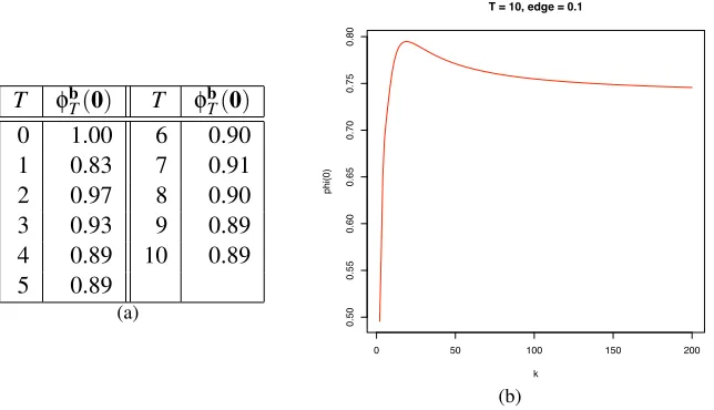
. Using a different initial distribution, Schapire and Singer (1999) achieve the slightly better bound p(k−1)e−Tγ2/2. However, when the edge γis small and the number of rounds are few, each bound is greater than 1 and hence trivial. On the other hand, the bounds computed by the above dynamic program are sensible for all values ofk, γandT. Whenbis theγ-biased uniform distributionb= (1−kγ+γ,1−kγ,1−kγ, . . . ,1−kγ)a table containing the error upper boundφb
T(0)fork=6,
γ=0 and small values for the number of rounds T is shown in Figure 2(a); note that with the exponential loss, the bound is always 1 if the edgeγis 0. Further, the bounds due to the exponential loss analyses seem to imply that the dependence of the error on the number of labels is monotonic. However, a plot of the tighter bounds with edgeγ=0.1, number of roundsT =10 against various values ofk, shown in Figure 2(b), indicates that the true dependence is more complicated. Therefore the tighter analysis also provides qualitative insights not obtainable via the exponential loss bound.
7. Solving for the Minimal Weak Learning Condition
In the previous section we saw how to find the optimal boosting strategy when using any fixed edge-over-random condition. However as we have seen before, these conditions can be stronger than necessary, and therefore lead to boosting algorithms that require additional assumptions. Here we show how to compute the optimal algorithm while using the weakest weak learning condition, provided by (13), or equivalently the condition used by AdaBoost.MR,(
C
MR,BMRT φb
T(0) T φbT(0) 0 1.00 6 0.90 1 0.83 7 0.91 2 0.97 8 0.90 3 0.93 9 0.89 4 0.89 10 0.89 5 0.89
(a)
0 50 100 150 200
0
.5
0
0
.5
5
0
.6
0
0
.6
5
0
.7
0
0
.7
5
0
.8
0
T = 10, edge = 0.1
k
p
h
i(0
)
(b)
Figure 2: Plot of potential value φb
T(0)where bis the γ-biased uniform distribution: b= ( 1−γ
k +
γ,1−kγ,1−kγ, . . . ,1−kγ). (a): Potential values (rounded to two decimal places) for different number of roundsT usingγ=0 andk=6. These are bounds on the error, and less than 1 even when the edge and number of rounds are small.(b): Potential values for different number of classesk, withγ=0.1, andT =10. These are tight estimates for the optimal error, and yet not monotonic in the number of classes.
7.1 Game-theoretic Equivalence of Necessary and Sufficient Weak-learning Conditions In this section we study the effect of the weak learning condition on the game-theoretically optimal boosting strategy. We introduce the notion ofgame-theoretic equivalencebetween two weak learn-ing conditions, that determines if the payoffs (15) of the optimal boostlearn-ing strategies based on the two conditions are identical. This should hold whenever both games last for the same number of iterationsT, for any value ofT. This is different from the usual notion of equivalence between two conditions, which holds if any weak classifier space satisfies both conditions or neither condition. In fact we prove that game-theoretic equivalence is a broader notion; in other words, equivalence implies game-theoretic equivalence. A special case of this general result is that any two weak learning conditions that are necessary and sufficient, and hence equivalent to boostability, are also game-theoretically equivalent. In particular, so are the conditions of AdaBoost.MR and (13), and the resulting optimal Booster strategies enjoy equally good payoffs. We conclude that in order to derive the optimal boosting strategy that uses the minimal weak-learning condition, it is sound to use either of these two formulations.
The purpose of a weak learning condition(
C
,B)is to impose restrictions on the Weak-Learner’s responses in each round. These restrictions are captured by subsets of the weak classifier space as follows. If Booster chooses cost-matrix C∈C
in a round, the Weak-Learner’s response h is restricted to the subsetSC⊆H
alldefined asSC=