Asymptotic Results on Adaptive False Discovery Rate Controlling
Procedures Based on Kernel Estimators
Pierre Neuvial∗ PIERRE.NEUVIAL@GENOPOLE.CNRS.FR
Laboratoire Statistique et Génome Université d’Évry Val d’Essonne UMR CNRS 8071 – USC INRA 23 boulevard de France 91 037 Évry, France
Editor:Olivier Teytaud
Abstract
The False Discovery Rate (FDR) is a commonly used type I error rate in multiple testing problems. It is defined as the expected False Discovery Proportion (FDP), that is, the expected fraction of false positives among rejected hypotheses. When the hypotheses are independent, the Benjamini-Hochberg procedure achieves FDR control at any pre-specified level. By construction, FDR control offers no guarantee in terms of power, or type II error. A number of alternative procedures have been developed, including plug-in procedures that aim at gaining power by incorporating an estimate of the proportion of true null hypotheses.
In this paper, we study the asymptotic behavior of a class of plug-in procedures based on kernel estimators of the density of the p-values, as the number mof tested hypotheses grows to infinity. In a setting where the hypotheses tested are independent, we prove that these procedures are asymptotically more powerful in two respects: (i) a tighter asymptotic FDR control for any target FDR level and (ii) a broader range of target levels yielding positive asymptotic power. We also show that this increased asymptotic power comes at the price of slower, non-parametric convergence rates for the FDP. These rates are of the formm−k/(2k+1), wherekis determined by the regularity of the density of thep-value distribution, or, equivalently, of the test statistics distribution. These results are applied to one- and two-sided tests statistics for Gaussian and Laplace location models, and for the Student model.
Keywords: multiple testing, false discovery rate, Benjamini Hochberg’s procedure, power, crit-icality, plug-in procedures, adaptive control, test statistics distribution, convergence rates, kernel estimators
1. Introduction
Multiple simultaneous hypothesis testing has become a major issue for high-dimensional data analy-sis in a variety of fields, including non-parametric estimation by wavelet methods in image analyanaly-sis, functional magnetic resonance imaging (fMRI) in medicine, source detection in astronomy, and DNA microarray or high-throughput sequencing analyses in genomics. Given a set of observations corresponding either to a null hypothesis or an alternative hypothesis, the goal of multiple testing is to infer which of them correspond to true alternatives. This requires the definition of risk measures
that are adapted to the large number of tests performed: typically 104to 106in genomics. The False
Discovery Rate (FDR) introduced by Benjamini and Hochberg (1995) is one of the most commonly used and one of the most widely studied such risk measure in large-scale multiple testing prob-lems. The FDR is defined as the expected proportion of false positives among rejected hypotheses. A simple procedure called the Benjamini-Hochberg (BH) procedure provides FDR control when the tested hypotheses are independent (Benjamini and Hochberg, 1995) or follow specific types of positive dependence (Benjamini and Yekutieli, 2001).
When the hypotheses tested are independent, applying the BH procedure at levelαin fact yields FDR=π0α, whereπ0 is the unknown fraction of true null hypotheses (Benjamini and Yekutieli,
2001). This has motivated the development of a number of “plug-in” procedures, which consist in applying the BH procedure at levelα/πˆ0, where ˆπ0is an estimator ofπ0. A typical example is the
Storey-λprocedure (Storey, 2002; Storey et al., 2004) in which ˆπ0 is a function of the empirical
cumulative distribution function of thep-values.
In this paper, we consider an asymptotic framework where the numbermof tests performed goes to infinity. When ˆπ0converges in probability toπ0,∞∈[π0,1)asm→+∞, the corresponding
plug-in procedure is by construction asymptotically more powerful than the BH procedure, while still providing FDR≤α. However, as FDR control only implies that theexpectedFDP is below the target level, it is of interest to study thefluctuationsof the FDP achieved by such plug-in procedures around their corresponding FDR. This paper studies the influence of the plug-in step on the asymptotic properties of the corresponding procedure for a particular class of estimators ofπ0, which may be
written as kernel estimators of the density of the p-value distribution at 1.
2. Background and Notation
In this section, we introduce the multiple testing setting considered in this paper, and define two central concepts: plug-in procedures and criticality.
2.1 Multiple Testing Setting
We consider a test statistic X distributed as F0 under a null hypothesis
H
0 and as F1 under analternative hypothesis
H
1. We assume that for a∈ {0,1}, Fa is continuously differentiable, and that the corresponding density function, which we denote by fa, is positive. This testing problem may be formulated in terms of p-values instead of test statistics. The p-value function is defined as p:x7→PH0(X≥x) =1−F0(x) for one-sided tests and p:x7→PH0(|X| ≥ |x|) for two-sidedtests. AsF0is continuous, thep-values are uniform on[0,1]under
H
0. For consistency we denoteby G0 the corresponding distribution function, that is, the identity function on [0,1]. Under
H
1,the distribution function and density of the p-values are denoted byG1andg1, respectively. Their expression as functions of the distribution of the test statistics are recalled in Proposition 1 below in the case of one- and two-sidedp-values. For two-sided p-values, we assume that the distribution function of the test statistics under
H
0is symmetric (around 0):∀x∈R,F0(x) +F0(−x) =1. (1)
Assumption (1) is typically satisfied in usual models such as Gaussian or Laplace (double exponen-tial) models. Under Assumption (1), the two-sided p-value satisfies p(x) =2(1−F0(|x|))for any
Proposition 1 (One- and two-sidedp-values) For t∈[0,1], let q0(t) =F0−1(1−t). The distribu-tion funcdistribu-tion G1and the and density function g1of the p-value under
H
1at t satisfy the following:1. for a one-sided p-value, G1(t) =1−F1(q0(t))and g1(t) = (f1/f0) (q0(t)); 2. for a two-sided p-value, G1(t) =1−F1(q0(t/2)) +F1(−q0(t/2))and
g1(t) =1/2((f1/f0) (q0(t/2)) + (f1/f0) (−q0(t/2))).
The assumption that f1is positive entails thatg1is positive as well. We further assume that
G1is concave. (2)
Asg1is a function of the likelihood ratio f1/f0and the non-increasing functionq0, Assumption (2)
may be characterized as follows:
Lemma 2 (Concavity and likelihood ratios) 1. For a one-sided p-value, Assumption(2)holds
if and only if the likelihood ratio f1/f0is non-decreasing.
2. For a two-sided p-value under Assumption (1), Assumption (2) holds if and only if x7→
(f1/f0)(x) + (f1/f0)(−x)is non-decreasing onR+.
We consider a sequence of independent tests performed as described above and indexed by the setN∗of positive integers. We assume that either all of them are one-sided tests, or all of them are
two-sided tests. This sequence of tests is characterized by a sequence(H,p) = (Hi,pi)i∈N∗ , where for eachi∈N∗, piis a p-value associated to theithtest, andHiis a binary indicator defined by
Hi=
(
0 if
H
0is true for testi 1 ifH
1is true for testi .We also letm0(m) =∑mi=1(1−Hi), andπ0,m=m0(m)/m. Following the terminology proposed by Roquain and Villers (2011), we define theconditional settingas the situation whereHis deter-ministic andpis a sequence of independent random variables such that fori∈N∗,pi∼GH
i. This is a particular case of the setting originally considered by Benjamini and Hochberg (1995), where no assumption was made on the distribution of pi when Hi=1. In the present paper, we consider an
unconditional settingintroduced by Efron et al. (2001), which is also known as the “random effects” setting. Specifically,His a sequence of random indicators, independently and identically distributed as
B
(1−π0), whereπ0∈(0,1), and conditional onH,pfollows the conditional setting, that is, the p-values satisfy pi|Hi∼GHi. This unconditional setting has been widely used in the multiple test-ing literature, see, for example, Storey (2003); Genovese and Wasserman (2004); Chi (2007a). In this setting, the p-values are independently, identically distributed asG=π0G0+ (1−π0)G1, and m0(m)follows the binomial distributionBin(m,π0).Remark 3 We are assuming thatπ0<1, which implies that the proportion 1−π0,m of true null
As G0 is the identity function, the multiple testing model is entirely characterized by the two
parametersπ0 andG1 (or, equivalently,π0 andG), whereG1 is itself entirely characterized byF0
andF1, by Proposition 1. The mixture distributionGis concave if and only if Assumption (2) holds.
More generally, we note that making a regularity assumption onG1(org1) is equivalent to making
the same regularity assumption onG(org):
Remark 4 (Differentiability assumptions) Throughout the paper, differentiability assumptions on
the distribution of the p-values near 1 are expressed in terms of g, the (mixture) p-value density. As g=π0+ (1−π0)g1, we note that they could equally be written in terms of g1, the p-value density under the alternative hypothesis.
2.2 Type I and II Error Rate Control in Multiple Testing
We define a multiple testing procedure
P
as a collection of functions (P
α)α∈[0,1]such that for anyα∈[0,1],
P
αtakes as input a vector ofm p-values, and returns a subset of{1, . . .m}corresponding to the indices of hypotheses to be rejected. For a given procedureP
and a givenα∈[0,1], the functionP
αwill be called “ProcedureP
at (target) levelα”. In this paper, we focus onthresholding-based multiple testing procedures, for which the rejected hypotheses are those with p-values less than a threshold. Each possible value for the threshold corresponds to a trade-off between false positives (type I errors) and false negatives (type II errors). Most risk measures developed for multiple testing procedures are based on type I errors. We focus on one such measure, the False Discovery Rate (FDR), which is one of the most widely used error rate in multiple testing. Denoting byRm be the total number of rejections ofP
α amongmhypotheses tested, and byVm the number of false rejections, the corresponding False Discovery Proportion is defined as FDPm=Vm/(Rm∨1), and the False Discovery Rate is the expected FDP, that is:FDRm=E
Vm
Rm∨1
.
A trivial way to control the FDR, or any risk measure only based on type I errors, is to make no rejection with high probability. Obviously, this is not the best strategy, as it may lead to a high number of type II errors. The performance of multiple testing procedures may be evaluated through their power, which is a function of the number of type II errors. Specifically, the power of a multiple testing procedure at level α is generally defined as the (random) proportion of correct rejections (true positives) among true alternative hypotheses (see, for example, Chi, 2007a):
Πm= Rm−Vm (m−m0(m))∨1.
Remark 5 All of the quantities defined in this section implicitly depend on the multiple testing
procedure considered,
P
= (P
α)α∈[0,1]. However, for simplicity, we will write Rm,Vm,FDRm, and Πm, instead of RPαm ,VmPα,FDRmPα, andΠPmαwhenever not ambiguous.
Remark 6 By definition, the power of a thresholding-based procedure is a non-decreasing
2.3 The Benjamini-Hochberg Procedure
Suppose we wish to control the FDR at level α. Let p(1)≤. . .≤ p(m) be the ordered p-values,
and denote by H(i) the null hypothesis corresponding to p(i). Define bIm(α) as the largest index
k≥0 such that p(k)≤αk/m. The Benjamini-Hochberg procedure at levelαrejects all H(i) such
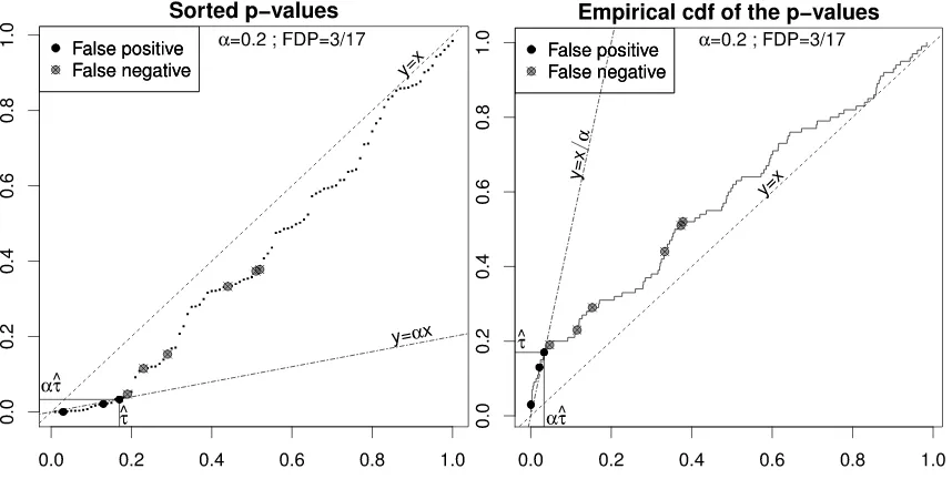
that i≤Ibm(α) (if Ibm(α) =0, then no rejection is made). This procedure has been proposed by Benjamini and Hochberg (1995) in the context of FDR control; Seeger (1968) reported that it had previously been used by Eklund (1961–1963) in another multiple testing context. When all true null hypotheses are independent, the BH procedure at level αyields strongFDR control, that is, it entails FDR≤α regardless of the number of true null hypotheses (Benjamini and Hochberg, 1995). The BH procedure also controls the FDR when thep-values satisfy specific forms of positive dependence, see Benjamini and Yekutieli (2001). Figure 1 illustrates the application of the BH procedure withα=0.2 tom=100 simulated hypotheses, among which 20 are true alternatives. The left panel illustrates the above definition of the BH procedure. An equivalent definition is that the procedure rejects all hypotheses with associatedp-value is less thanbτm(α) =αbIm(α)/m. The
Figure 1: Illustrations of the BH procedure on a simulated example with m=100. Left: sorted
p-values: i/m7→p(i). Right: empirical distribution function:t7→Gbm(t).
right panel provides a dual representation of the same information, where the x andy axes have been swapped. It gives a geometrical interpretation ofbτm(α)as the largest crossing point between the line y=x/α and the empirical distribution function of the p-values, defined fort∈[0,1]by
b
Gm(t) =∑mi=11P
i≤t:
bτm(α) =sup{t∈[0,1],Gbm(t)≥t/α}.
2.4 Plug-in Procedures
and Hochberg, 1995; Benjamini and Yekutieli, 2001). This entails that the BH(α′)procedure yields
FDR≤αif and only ifα′≤α/π0. Therefore, as the threshold of the BH(α) procedure is a
non-decreasing function ofαand by Remark 6, the BH(α/π0)procedure is optimal in our setting, in the
sense that it yields maximum power among procedures of the form BH(α′)that control the FDR at
levelα. Asπ0is unknown, this procedure cannot be implemented; it is generally referred to as the
Oracle BH procedure.
Remark 7 Ifα≥π0, then rejecting all null hypotheses is optimal, as it corresponds to the largest possible threshold while still maintainingFDR=π0≤α. Therefore, we will assume that α<π0 throughout the paper.
In order to mimic the Oracle procedure, it is natural to apply the BH procedure at levelα/πˆ0,m, where ˆπ0,m≤1 is an estimator ofπ0 (Benjamini and Hochberg, 2000). Such plug-in procedures
(also known as two-stage adaptive procedures) have the same geometric interpretation as the BH procedure (see Figure 1) in terms of the largest crossing point, with α/πˆ0,m instead ofα. Their rejection threshold can be written asbτ0
m(α) =bτm(α/πˆ0,m), that is:
bτ0
m(α) =sup{t∈[0,1],Gbm(t)≥πˆ0,mt/α}. Note thatbτ0
mdepends on the observations through both Gbm and ˆπ0,m. By construction, a plug-in procedure based on an estimator ˆπ0,mthat converges in probability toπ0,∞∈[π0,1)asm→+∞is
asymptotically more powerful that the original BH procedure.
Adapting a method originally proposed by Schweder and Spjøtvoll (1982), Storey (2002) de-fined ˆπSto
0,m(λ) =#{i/Pi≥λ}/#{i≥λ}forλ∈(0,1). This estimator is generally referred to as the Storey-λestimator. It may also be written as a function of the empirical distribution of thep-values:
ˆ πSto
0,m(λ) =
1−Gbm(λ)
1−λ . (3)
The rationale for ˆπSto
0,m(λ) is that under Assumption (2), larger p-values are more likely to cor-respond to true null hypotheses than smaller ones. Moreover, ˆπSto
0,m(λ)converges in probability to (1−G(λ))/(1−λ), where the limit is greater thanπ0asGstochastically dominates the uniform
dis-tribution. Several choices ofλhave been proposed, includingλ=1/2 (Storey and Tibshirani, 2003), a data-driven choice based on the bootstrap (Storey et al., 2004), andλ=α(Blanchard and Roquain, 2009). In our setting, a slightly modified version of the corresponding plug-in BH(α/πˆSto
0,m(λ)) pro-cedure where 1/mis added to the numerator in (3) achieves strong FDR control at levelα(Storey et al., 2004). We note that the Storey-λestimator ˆπSto
0,m(λ)can be viewed as a kernel estimator of the densitygat 1.
Definition 8 (Kernel of orderℓand kernel estimator of a density at a point)
1. A kernel of order ℓ∈N is a function K:R→R such that the functions u7→ujK(u) are
integrable for any j=0. . . ℓ, and satisfyRRK=1, and R
RujK(u)du=0for j=1. . . ℓ. 2. The kernel estimator of a density g at x0 based on m independent, identically distributed
observations x1, . . .xmfrom g is defined by
ˆ
gm(x0) =
1
mh
m
∑
i=1 K
x
i−x0 h
,
By Definition 8, ˆπSto
0,m(λ)is a kernel estimator of the density gat 1 with kernelKSto(t) =1[−1,0](t)
and bandwidthh=1−λ. KStois an asymmetric, rectangular kernel of order 0. 2.5 Criticality and Asymptotic Properties of FDR Controlling Procedures
Upper bounds on the asymptotic number of rejections of FDR controlling procedures have been identified and characterized by Chi (2007a) and Chi and Tan (2008), who introduced the notion of
critical value of a multiple testing problemand that ofcritical value of a multiple testing procedure. Both notions are defined formally below. They are tightly connected, with the important difference that the former only depends on the multiple testing problem, while the latter depends on both the multiple testing problem and a specific multiple testing procedure.
Definition 9 (Critical value of a multiple testing problem) The critical value of the multiple
test-ing problem parametrized byπ0and G is defined by
α⋆= inf t∈(0,1]
π0t
G(t). (4)
Chi and Tan (2008, proof of Proposition 3.2) proved that for any multiple testing procedure, for α<α⋆, there exists a positive constantc(α)such that almost surely, formlarge enough, the events
{Vm/Rm≤α}and{Rm≥c(α)logm}are incompatible. This restriction is intrinsic to the multiple testing problem, in the sense that it holds regardless of the considered multiple testing procedure. Obviously, this is not a limitation whenα⋆=0. We introduce the following Condition:
α⋆>0. (5)
Whether Condition (5) is satisfied or not only depends onG. However, the value ofα⋆as defined
in (4) depends on bothπ0andG. Under Assumption (2) we haveα⋆=limt→0π0t/G(t) =π0/(π0+
(1−π0)g1(0)), whereg1(0)∈[0,+∞]is defined byg1(0) =limt→0g1(t). By Proposition 1,g1(0)
only depends on the behavior of the test statistics distribution. In particular, under Assumption (2), Condition (5) is satisfied if and only if the likelihood ratio f1/f0is bounded near+∞.
We now introduce the notion of critical value of a multiple testing procedure. Chi (2007a) defined the critical value of the BH procedure asα⋆BH=inft∈(0,1]t/G(t). Let us denote by
τ∞(α) =sup{t∈[0,1],G(t)≥t/α} (6)
the rightmost crossing point betweenGand the liney=x/α. Chi (2007a) has proved the following result:
Proposition 10 (Asymptotic properties of the BH procedure) For α ∈[0,1], let bτm(α) be the
threshold of the BH(α) procedure, and let τ∞(α) be defined by (6). Let αBH⋆ =inft∈(0,1]t/G(t). As m→+∞,
1. Ifα<α⋆
BH, thenbτm(α)a→.s.0;
2. Ifα>α⋆
A straightforward consequence of Proposition 10 is that the BH(α) procedure has asymptotically null power whenα<α⋆BH and positive power whenα>α⋆BH. The following Definition generalizes the notion of critical value of to a generic multiple testing procedure:
Definition 11 (Critical value of a multiple testing procedure) Let
P
denote a multiple testing pro-cedure. The critical value ofP
is defined byα⋆P =sup
α∈[0,1],ΠPα
m a.s.
−→
m→+∞0
.
The critical value α⋆
P depends on both the procedure
P
, and the multiple setting. For the BHprocedure, criticality (α<α⋆BH) corresponds to situations where the target FDR levelαis so small that there is no positive crossing point betweenG and the liney=x/α. Conversely, when α> α⋆
BH, there is a positive crossing point betweenGand the line y=x/α, as illustrated by Figure 1 (right). The almost sure convergence results of Proposition 10 in the caseα>α⋆BHwere extended by Neuvial (2008), in the conditional setting. Specifically, the thresholdbτm(α)of the BH procedure was shown to converge in distribution toτ∞(α)at ratem−1/2as soon asα>α⋆BH. Neuvial (2008) also proved that similar central limit theorems hold for a class of thresholding-based FDR controlling procedures that covers some plug-in procedures, including the Storey-λprocedure: the threshold of a procedure
P
of this class converges in distribution to a procedure-specific, positive value at ratem−1/2as soon asα>α⋆ P.
Remark 12 (Criticality of a multiple testing problem versus criticality of a procedure) Whether
Condition(5)hols or not only depends on the behavior of the test statistics distribution. However,
this condition is tightly connected to the critical value of FDR controlling procedures. In order to shed some light on this connection, we note thatα⋆=π0α⋆BH may be interpreted as the critical
value of the Oracle BH procedure BH(α/π0). Therefore, as the Oracle BH procedure at level α is the most powerful procedure among thresholding-based procedures that control FDR at levelα,
α⋆ is a lower bound on the critical values of these procedures. Specifically, multiple problems for which Condition(5)is satisfied or not differ in that:
• when Condition(5)is satisfied, all thresholding-based procedures that control FDR have null
asymptotic power in a range of levels containing[0,α⋆);
• when Condition(5)is not satisfied, some procedures (including BH) have positive asymptotic
power for any positive levelα.
This paper extends the asymptotic results of Chi (2007a) and Neuvial (2008) to the case of plug-in procedures of the form BH(α/πˆ0,m), where ˆπ0,mis a kernel estimator of thep-value distribution
gat 1. Specifically, we consider a class of kernel estimators ofπ0, which includes a modification
of the Storey-λestimator, where the parameterλtends to 1 asm→∞. In Section 3, we prove that this class of estimators ofπ0achieves non-parametric convergence rates of the formm−k/(2k+1)/ηm, whereηmgoes to 0 slowly enough asm→+∞, andkcontrols the regularity ofgat 1. In Section 4, we characterize the critical valueα⋆
0of plug-in procedures based on such estimators, and prove that
when the target FDR level αis greater thanα⋆
0, the convergence rate of these plug-in procedures
3. Asymptotic Properties of Non-Parametric Estimators ofπ0
Letλ∈(0,1). The expectationπ0(λ)of the Storey-λestimator is given by
π0(λ) =π0+ (1−π0)
1−G1(λ)
1−λ . (7)
Moreover, as a regular function of the empirical distribution of thep-values, ˆπSto
0,m(λ)has the follow-ing asymptotic distribution forλ∈(0,1)(Genovese and Wasserman, 2004):
√m
ˆ πSto
0,m(λ)−π0(λ)
N
0,G(λ)(1−G(λ)) (1−λ)2
.
In our setting,g1is positive, as noted in Section 2.1. Therefore, we haveG1(λ)<1 for anyλ∈ (0,1), and the biasπ0(λ)−π0is positive: the Storey-λestimator achieves a parametric convergence
rate, but it is not a consistent estimator of π0. Under Assumption (2), this bias decreases as λ
increases (by Equation (7)). In order to mimic the Oracle BH(α/π0)procedure, it is therefore natural
to chooseλclose to 1. We consider plug-in procedures whereπ0is estimated by ˆπ0,Stom(1−hm), with
hm→0 asm→+∞. As the limit in probability of this estimator isg(1) =π0+ (1−π0)g1(1), it is
consistent if and only if the following “purity” condition, which has been introduced by Genovese and Wasserman (2004), is met:
g1(1) =0 (8)
We note that the Storey-λestimator is not a consistent estimator ofπ0 even in when Condition (8)
is met. Moreover, Condition (8) is entirely determined by the shape of the test statistics under the alternative hypothesis. The asymptotic bias and variance of ˆπSto
0,m(1−hm) are characterized by Proposition 13:
Proposition 13 (Asymptotic bias and variance ofπˆSto
0,m(1−hm)) Let (hm)m∈N be a positive sequence such that hm→0.
1. If mhm→+∞as m→+∞, then
p
mhm πˆSto0,m(1−hm)−EπˆSto0,m(1−hm)
N
(0,g(1)).2. Assume that for k≥1, g is k times differentiable at1, with g(l)(1) =0for1≤l<k. Then
EπˆSto
0,m(1−hm)−g(1)m=
→+∞
(−1)kg(k)(1)
(k+1)! h k m+o
hkm.
Only the bias term in Proposition 13 depends on the regularity k of the distribution near 1: the asymptotic bias is of orderhkm, while the asymptotic variance of ˆπSto
0,m(1−hm)is of order(mhm)−1, regardless of the regularity of the distribution. The bandwidthhmin Proposition 13 realizes a trade-off between the asymptotic bias and variance of ˆπSto
Proposition 14 (Asymptotic properties ofπˆSto
0,m(1−hm)) Assume that g is k times differentiable at 1for k≥1, with g(l)(1) =0for1≤l<k.
1. If g(k)(1)6=0, then the asymptotically optimal bandwidth forπˆSto
0,m(1−hm)in terms of MSE is
of order m−1/(2k+1), and the corresponding MSE is of order m−2k/(2k+1).
2. Letηmbe any sequence such thatηm→0and mk/(2k+1)ηm→+∞as m→+∞. Then, letting hm(k) =m−1/(2k+1)η2m, we have, as m→+∞:
mk/(2k+1)η
m πˆSto0,m(1−hm(k))−g(1)
N
(0,g(1)). (9) Proposition 14 is proved in Appendix B. The convergence rate in (9) is a typical convergence rate for non-parametric estimators of a density at a point. However, Proposition 14 cannot be derived from classical results on kernel estimators such as those obtained in Tsybakov (2009). Indeed, such results typically require that the order of the kernel matches the regularitykof the density, whereas the kernel of Storey’s estimator,KSto(t) =1[−1,0](t), is of order 0. The results that can be obtained with kernels of orderkare summarized by Proposition 15; we refer to Tsybakov (2009) for a proof of this result.Proposition 15 (kthorder kernel estimator) Assume that for k≥1, g is k times differentiable at1.
Letgˆkm(1)be a kernel estimator of g(1)with bandwidth hm, associated with a kthorder kernel.
1. The optimal bandwidth forgˆkm(1)in terms of MSE is of order m−1/(2k+1), and the
correspond-ing MSE is of order m−2k/(2k+1);
2. Letηmbe any sequence such thatηm→0and mk/(2k+1)ηm→+∞as m→+∞. Then letting
hm(k) =m−1/(2k+1)η2m, we have, as m→+∞:
mk/(2k+1)η
m
ˆ
gkm(1)−g(1)
N
(0,g(1)).Propositions 14 and 15 show that the convergence rate of kernel estimators ofg(1)with asymp-totically optimal bandwidth directly depends on the regularity k of g at 1. The only difference between the two propositions is that the assumption that the firstk−1 derivatives ofgare null at 1 for ˆπ0,m(1−hm)is not needed forkth order kernel estimators. Importantly, these convergence rates cannot be improved in our setting, in the sense thatm−k/(2k+1)is the minimax rate for the estimation of a density at a point where its regularity is of orderk(Tsybakov, 2009, Chapter 2).
To the best of our knowledge, the only non-parametric estimators ofπ0 for which convergence
rates have been established in our setting are those proposed by Storey (2002), Swanepoel (1999) and Hengartner and Stark (1995). We now briefly review asymptotic properties of these estimators in the context of multiple testing, as stated in Genovese and Wasserman (2004), and show that their convergence rates can essentially be recovered by Propositions 14 and 15.
Confidence envelopes for the density: Hengartner and Stark (1995) derived a finite sample confi-dence envelope for a monotone density. Assuming thatGis concave and thatgis Lipschitz in a neighborhood of 1, Genovese and Wasserman (2004) obtained an estimator which con-verged to g(1) at rate (lnm)1/3m−1/3. The same rate of convergence can be achieved by
Spacings-based estimator: Swanepoel (1999) proposed a two-step estimator of the minimum of an unknown density based on the distribution of the spacings between observations: first, the location of the minimum is estimated, and then the density at this point is itself estimated. Assuming that at the value at which the densitygachieves its minimum,gandg(1)are null,
andg(2) is bounded away from 0 and+∞and Lipschitz, then for any δ>0, there exists an estimator converging at rate(lnm)δm−2/5to the true minimum. The same rate of convergence
can be achieved by Proposition 14 or 15 (forηm= (lnm)−δ) if one assumes thatg is twice differentiable at 1 (and additionally thatg(1)(1) =0 for Proposition 14). In our setting, the Lipschitz condition for the second derivative is unnecessary: the minimum ofgis necessarily achieved at 1 because g is non-increasing (under Assumption (2)), so the first step of the estimation in Swanepoel (1999) may be omitted.
As both estimators are estimators ofg(1), the differences in their asymptotic properties are driven by the differences in the regularity assumptions made forg(org1) near 1, rather than by their specific
form.
4. Consistency, Criticality and Convergence Rates of Plug-in Procedures
The aim of this section is to derive convergence rates for plug-in procedures based on the estima-tors ˆπ0,m ofπ0 studied in Section 3. Specifically, our goal is to establish central limit theorems
for the thresholdbτ0
m(α) of the plug-in procedure BH(α/πˆ0,m) and the associated False Discov-ery Proportion, which we denote by FDPm(bτ0m(α)). The convergence results obtained by Neuvial (2008) cover a broad class of FDR controlling procedures, including the BH procedure and plug-in procedures based on estimators of π0 that depend on the observations only through the empirical
distribution functionGbmof the p-values (Storey, 2002; Storey et al., 2004; Benjamini et al., 2006).
Although these results were obtained in the conditional setting of Benjamini and Hochberg (1995), extending them to the unconditional setting considered here is relatively straightforward, because the proof techniques developed in Neuvial (2008) can be adapted to this setting. For completeness, the asymptotic properties of the BH procedure and the plug-in procedure based on the Storey-λ estimator are derived in Appendix C. The problem considered in this section is more challenging, as the kernel estimators introduced in Section 3 depend onmnot only throughGbm, but also through
the bandwidth of the kernel (for example,hmfor ˆπSto0,m(1−hm)).
Let ˆπ0,m denote a generic estimator of π0. We assume that ˆπ0,m converges in probability to π0,∞≤1 as m→+∞. We do not assume that π0,∞=π0. Therefore, ˆπ0,m may or may not be a consistent estimator of π0. We recall that the BH(α/πˆ0,m) procedure rejects all hypotheses with
p-values smaller than b
τ0
m(α) =sup
n
t∈[0,1],Gbm(t)≥πˆ0,mt/αo.
We now study the behavior of the BH(α/πˆ0,m)procedure when ˆπ0,mconverges at a ratermslower than the parametric ratem−1/2, that is,m−1/2=o(rm). We define the asymptotic thresholdτ0∞(α) corresponding tobτ0
m(α)as
τ0
∞(α) =sup{t∈[0,1],G(t)≥π0,∞t/α}.
We have τ0
Theorem 16 (Asymptotic properties of plug-in procedures) Letπˆ0,mbe an estimator ofπ0such thatπˆ0,m→π0,∞in probability as m→+∞. Letα⋆0=π0,∞α⋆BH. Then:
1. α⋆0is the critical value of the BH(α/πˆ0,m)procedure;
2. Further assume that the asymptotic distribution ofπˆ0,mis given by
p
mhm(πˆ0,m−π0,∞)
N
(0,s20)for some s0, with hm=o(1/ln lnm)and mhm→+∞as m→+∞. Then, under Assumption(2),
for anyα>α⋆ 0,
(a) The asymptotic distribution of the thresholdbτ0
m(α)is given by
p
mhm bτ0m(α)−τ0∞(α)
N
0,s
0τ0∞(α)/α
π0,∞/α−g(τ0∞(α)) 2!
;
(b) The asymptotic distribution of the FDP achieved by the BH(α/πˆ0,m)procedure is given
by
p
mhm
FDPm(bτ0m(α))− π0α
π0,∞
N
0, π0αs0 π2
0,∞ !2
.
Theorem 16 states that forα>α⋆
0, for any estimator ˆπ0,mthat converges in distribution at a rate rm slower than the parametric ratem−1/2, the plug-in procedure BH(α/πˆ0,m) converges at raterm as well. This is a consequence of the fact thatrm dominates the fluctuations ofGbm, which are of parametric order.
We now state the main result of the paper (Corollary 17), that is, the asymptotic properties of plug-in procedures associated with the estimators ofπ0 studied in Section 3, for whichs20=g(1).
This result can be derived by combining the results of Theorem 16 with those of Propositions 14 and 15.
Corollary 17 Assume that (2) holds, and that g is k times differentiable at 1 for k≥1. Define
hm(k) =m−1/(2k+1)η2m, whereηm→0and mk/(2k+1)ηm→+∞as m→+∞. Denote byπˆk0,mone of
the following two estimators ofπ0:
• Storey’s estimator πˆSto
0,m(1−hm(k)); in this case, it is further assumed that g(l)(1) =0 for 1≤l<k;
• A kernel estimator of g(1)associated with a kthorder kernel with bandwidth h
m(k).
Then 1. α⋆
0=g(1)α⋆BH is the critical value of the BH(α/πˆk0,m)procedure;
2. For anyα>α⋆0,
(a) The asymptotic distribution of the thresholdbτ0
m(α)is given by
mk/(2k+1)η
m bτ0m(α)−τ0∞(α)
N
0,
τ0
∞(α)/α
g(1)/α−g(τ0
∞(α))
2 g(1)
(b) The asymptotic distribution of the FDP achieved by the BH(α/πˆ0,m)procedure is given
by
mk/(2k+1)ηm
FDPm(bτ0m(α))− π0α g(1)
N
0,π
2 0α2 g(1)3
.
We note that unlike the modification of the Storey-λ estimator studied here, the estimators ofπ0
based on kernels of orderkdo not require the firstk−1 derivatives ofgat 1 to be null. Therefore, the latter are generally preferable to the former. Corollary 17 has the following consequences, which are also summarized in Table 1:
• Assume that Condition (8) is met. Then the asymptotic threshold of the BH(α/πˆ0,m) pro-cedure isτ∞(α/π0), that is, the asymptotic threshold of the Oracle procedure BH(α/π0). In
particular, the asymptotic FDP achieved by the estimators in Corollary 17 is then exactly α (and its asymptotic variance is α2/π
0), whereas the asymptotic FDP of the original BH
procedure isπ0α.
• We have
α⋆≤α⋆0≤αSto⋆ (λ)≤α⋆BH.
In models where Condition (5) is not satisfied, all the critical values in (4) are null, implying that all the corresponding procedures have positive power for any target FDR level. In models where Condition (5) is satisfied, all the critical values in (4) are positive, and (4) implies that the range of target FDR valuesα that yield asymptotically positive power is larger for the plug-in procedures studied in this paper than for the BH procedure or the Storey-λprocedure.
• We haveτ0
∞(α)≥τ0,∞λ(α)≥τ∞(α), where τ0,∞λ(α) denotes the asymptotic threshold of the Storey-λprocedure, which is formally defined and characterized in Appendix C. Therefore, as the power of a thresholding-based FDR controlling procedure is a non-decreasing function of its threshold (Remark 6), the asymptotic power of the BH(α/πˆ0,m) procedure is greater than that of both the Storey-λand the original BH procedures, even in the rangeα>α⋆
BH where all of them have positive asymptotic power.
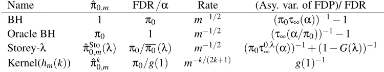
Name πˆ0,m FDR/α Rate (Asy. var. of FDP)/ FDR
BH 1 π0 m−1/2 (π0τ∞(α))−1−1
Oracle BH π0 1 m−1/2 (τ∞(α/π0))−1−1
Storey-λ πˆSto
0,m(λ) π0/π0(λ) m−1/2 (π0τ0,∞λ(α))−1+ (1−G(λ))−1 Kernel(hm(k)) πˆk0,m π0/g(1) m−k/(2k+1) g(1)−1
Table 1: Summary of the asymptotic properties of the FDR controlling procedures considered in this paper, for a target FDR levelα greater than the (procedure-specific) critical value. Note that “Storey-λ” denotes the original procedure with a fixed λ, while our extension withλ=1−hm(k)is categorized in the table as a particular case of kernel estimator (last row). For Storey-λ, we also assume thatλ>τ0,λ
∞ (α).
convergence rate. Specifically, the convergence rate of plug-in procedures is the non-parametric ratem−k/(2k+1)/ηm(wherekcontrols the regularity ofg) for the BH(α/πˆk0,m)procedure, while the parametric ratem−1/2 was achieved by the original BH procedure, the Oracle BH procedure, and the Storey-λprocedure (as proved in Appendix C).
5. Application to Location and Student Models
In Section 4 we proved that the asymptotic behavior of plug-in procedures depends on whether the target FDR level αis above or below the critical value α⋆0 characterized by Theorem 16, and by establishing convergence rates for these procedures whenα>α⋆
0. Both the critical valueα⋆0and the
obtained convergence rates depend on the test statistics distribution. In the present section, these results are applied to Gaussian and Laplace location models, and to the Student model. We begin by defining these models (Section 5.1) and studying criticality in each of them (Section 5.2). Then, we derive convergence rates for plug-in procedures based on the kernel estimators ofπ0considered
in Sections 3 and 4, both for two-sided tests (Section 5.3) and one-sided tests (Section 5.4).
5.1 Models for the Test Statistics
In this subsection, we define the location and Student models used throughout Section 5.
5.1.1 LOCATIONMODELS
In location models the distribution of the test statistic under
H
1is a shift from that of the test statistic underH
0: F1 =F0(· −θ) for some location parameterθ>0. The most widely studied locationmodels are the Gaussian and Laplace (double exponential) location models. Both the Gaussian and the Laplace distribution can be viewed as instances of a more general class of distributions introduced by Subbotin (1923) and given forγ≥1 by
f0γ(x) = 1
Cγ
e−|x|γ/γ
,withCγ=
Z +∞
−∞ e
−|x|γ/γ
dx=2Γ(1/γ)γ1/γ−1.
Therefore, the likelihood ratio in theγ-Subbotin location model may be written as
f1γ
f0γ(x) =exp
|x|γ
γ −
|x−θ|γ γ
. (10)
The Gaussian case corresponds to γ=2 and the Laplace case toγ=1. In the Laplace case, the distribution of the p-values under the alternative can be derived explicitly, see Lemma 22 in Ap-pendix. We focus on 1≤γ≤2 as this corresponds to situations in which Assumption (2) is satis-fied. Specifically, for one-sided tests, Assumption (2) holds as soon asγ≥1, because then f1γ/f0γis non-decreasing; for two-sided tests, if additionallyγ≤2, then Assumption (2) holds (as proved in Appendix A, Proposition 23).
5.1.2 STUDENT MODEL
Student’stdistribution is widely used in applications, as it naturally arises when testing equality of means of Gaussian random variables with unknown variance. In the Student model with parameter ν>0,F0 is the (central)t distribution withνdegrees of freedom, andF1 is the non-centralt
a location model, asF1 cannot be written as a translation of F0. Following Chi (2007a, Equation
(3.5)), we note that the likelihood ratio of the Student model may be written as
f1 f0
(t) =
+∞
∑
j=0
aj(ν,θ)ψ(j,ν)(t), (11)
whereψ(j,ν)(t) = (t/
√
t2+ν)j=sgn(t)j 1+ν/t2−j/2fort∈Rand
aj(ν,θ) =e−θ
2/2Γ((ν+j+1)/2)
Γ((ν+1)/2)
(√2θ)j
j! .
Remark 18 The sequence aj(ν,θ)is positive, and it is not hard to see that(∑jaj(ν,θ))is a
con-vergent series using Stirling’s formula. Therefore, asψ(j,ν)(t)∈[−1,1], the dominated convergence theorem ensures that the right-hand side of Equation(11)is well-defined for any t∈R.
Another useful expression for the Student likelihood ratio may be derived from the integral expression of the density of a non-centraltdistribution given by Johnson and Welch (1940):
f1
f0(t) =exp
"
−θ
2
2 1
1+tν2
#Hh ν
−√θt
ν+t2
Hhν(0)
, (12)
whereHhν(z) =R0+∞u ν
ν!e−
1
2(u+z)2dx. As noted by Chi (2007a, Section 3.1), the likelihood ratio of
Student test statistics is non-decreasing, which implies that Assumption (2) holds for one-sided tests. It also holds for two-sided tests, as proved in Appendix A, Proposition 26.
The location models and the Student model considered here are parametrized by two parameters: (i) a non-centrality parameter θ, which encodes a notion of distance between
H
0 andH
1; (ii) a parameter which controls the (common) tails of the distribution underH
0 andH
1: γ for the γ -Subbotin model, andνfor the Student model withνdegrees of freedom.5.2 Criticality
As the asymptotic behavior of plug-in procedures crucially depends on whether the target FDR level is above or below the critical valueα⋆0characterized by Theorem 16, it is of primary importance to study criticality in the models we are interested in. Noting thatα⋆
0=π0,∞α⋆BH=π0,∞α⋆/π0, we have
α⋆
0>0 if and only if Condition (5) is satisfied, that is, if and only if the likelihood ratio f1/f0 is
bounded near+∞. In this section, we study Condition (5) in location and Student models.
5.2.1 LOCATIONMODELS
In location models, where f1= f0(· −θ)withθ>0, the behavior of the likelihood ratio is closely related to the tail behavior of the distribution of the test statistics: for a given non-centrality param-eterθ, the heavier the tails, the smaller the difference between f1 and f0. In aγ-Subbotin location
model, Equation (10) yields|1−θ/x|γ∼1−γθ/xasx→+∞. Thus|x|γ 1− |1−θ/x|γ∼γθxγ−1,
and the behavior of the likelihood ratio f1γ/f0γis driven by the value ofγ, as illustrated by Figure 2 for the Gaussian and Laplace location models with location parameterθ∈ {1,2}.
Gaussian distribution (θ=1) Laplace distribution (θ=1)
0.0 0.2 0.4 0.6 0.8 1.0 0.0
0.2 0.4 0.6 0.8 1.0
p−value
π0=0
π0=0.5
π0=0.75
0.000000.0000 0.00010 0.00020
0.0005
0.0010
0.0015
0.0 0.2 0.4 0.6 0.8 1.0 0.0
0.2 0.4 0.6 0.8 1.0
p−value
π0=0
π0=0.5
π0=0.75
0.000000.00000 0.00010 0.00020
0.00005
0.00010
0.00015
Gaussian distribution (θ=2) Laplace distribution (θ=2)
0.0 0.2 0.4 0.6 0.8 1.0 0.0
0.2 0.4 0.6 0.8 1.0
p−value
π0=0
π0=0.5
π0=0.75
0.000000.000 0.00010 0.00020
0.005
0.010
0.015
0.020
0.0 0.2 0.4 0.6 0.8 1.0 0.0
0.2 0.4 0.6 0.8 1.0
p−value
π0=0
π0=0.5
π0=0.75
0.000000e+00 0.00010 0.00020
1e−04
2e−04
3e−04
Figure 2: Distribution functionsG for one-sided p-values (black) and two-sided p-values (gray), in Gaussian location models (left: Condition (5) is not satisfied), and Laplace location models (right: Condition (5) is satisfied) forπ0=0, 0.5 and 0.75. The location parameter
θis set to 1 in top panels and 2 in bottom panels. Inserted plot: zoom in the region
p<2.10−4.
anyθandπ0. This situation is illustrated by Figure 2 (left panels) for the Gaussian model (γ=2).
In such a situation, for any target FDR levelα, the asymptotic fraction of rejections by the BH(α)
procedure or by a plug-in procedure of the form BH(α/πˆ0,m), where ˆπ0,m→π0,∞in probability as
m→+∞, is positive by Lemma 27.
π0/(π0+ (1−π0)g1(0)), withg1(0) =eθfor one-sidedp-values, andg1(0) =coshθfor two-sided p-values. Laplace-distributed test statistics appear as a limit situation in terms of criticality: within the family ofγ-Subbotin location models withγ∈[1,2], the Laplace model (γ=1) is the only one for which Condition (5) is satisfied.
5.2.2 STUDENT MODEL
For the Student model, Equation (12) yields that (f1/f0)(t) converges to sν(θ) ast →+∞ and
sν(−θ)ast→ −∞, wheresν(θ) =Hhν(−θ)/Hhν(0)is positive for anyθ. Therefore, Condition (5) is satisfied for one-sided and two-sided tests in the Student model (this had already been noted by Chi (2007a) for one-sided tests). Figure 3 gives the distribution function of one- and two-sided
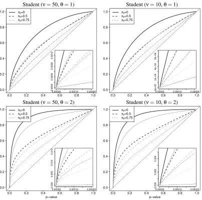
p-values in the Student model with parametersθ∈ {1,2}andν∈ {10,50}, forπ0∈ {0,0.5,0.75}.
Although criticality is much less obvious than for the Laplace model, the inserted plots which zoom into a region where thep-values are very small (p<2.10−4) do suggest forν=10 that the slope of
the distribution function has a finite limit at 0 for the Student model. As an illustration, we calculated that the critical values for one-sided tests in the Student model for π0=0.75 for θ∈ {1,2} are
respectively 0.173 and 0.015 forν=10, and 4.10−3and 7.10−6forν=50.
5.3 Two-Sided Tests
In this section we study consistency and convergence rates for two-sided tests.
5.3.1 CONSISTENCY
Let us first recall that by Proposition 1.2, we have for two-sided tests under a model satisfying Assumption (1):
g1(t) =1
2
f1
f0(q0(t/2)) + f1
f0(−q0(t/2))
, (13)
where q0:t7→F0−1(1−t) tends to 0 ast→1/2. A straightforward consequence of (13) is that g1(1) = (f1/f0)(0). As f1>0, we haveg(1) =π0+ (1−π0)g1(1)>π0. Therefore, Condition (8)
is not met, and the kernel estimators ofπ0studied in Section 3 are not consistent for the estimation
ofπ0. Specifically, we haveg1(1) =e−θ 2/2
for Gaussian and Student test statistics, andg1(1) =e−θ
for Laplace test statistics.
5.3.2 CONVERGENCERATES
Another consequence of (13) is that if fork≥1 the likelihood ratio f1/f0isktimes semi-differentiable
at 0, thengisktimes (left-)differentiable at 1. In particular, this holdsfor any kin theγ-Subbotin location model with γ∈[1,2], which covers the Gaussian and Laplace cases. It also holds for the Student model (as proved in Proposition 25). For these models, Corollary 17 entails that for any k>0, if ˆπ0,m is a kernel estimator of g associated with a kth order kernel with bandwidth
hm(k) =m−1/(2k+1)ηm2 (whereηm→0 andmηm→+∞asm→+∞), then the corresponding plug-in procedure BH(α/πˆ0,m) converges in distribution at rate m−k/(2k+1)/ηm for any α greater than α⋆
0=g(1)α⋆BH. These results are summarized in the last column of Table 2.
Let us now consider the modification of the Storey-λestimator introduced in Section 3: ˆπ0,m= ˆ
πSto
Student (ν=50,θ=1) Student (ν=10,θ=1)
0.0 0.2 0.4 0.6 0.8 1.0 0.0
0.2 0.4 0.6 0.8 1.0
p−value
π0=0
π0=0.5
π0=0.75
0.000000.0000 0.00010 0.00020
0.0004
0.0008
0.0012
0.0 0.2 0.4 0.6 0.8 1.0 0.0
0.2 0.4 0.6 0.8 1.0
p−value
π0=0
π0=0.5
π0=0.75
0.000000e+00 0.00010 0.00020
2e−04
4e−04
6e−04
Student (ν=50,θ=2) Student (ν=10,θ=2)
0.0 0.2 0.4 0.6 0.8 1.0 0.0
0.2 0.4 0.6 0.8 1.0
p−value
π0=0
π0=0.5
π0=0.75
0.000000.000 0.00010 0.00020
0.005
0.010
0.015
0.0 0.2 0.4 0.6 0.8 1.0 0.0
0.2 0.4 0.6 0.8 1.0
p−value
π0=0
π0=0.5
π0=0.75
0.000000.000 0.00010 0.00020
0.002
0.004
Figure 3: Distribution functionsGfor one-sidedp-values (black) and two-sided p-values (gray) in Student models withν=50 degrees of freedom (left) andν=10 (right). The location parameterθis set to 1 in top panels and 2 in bottom panels. Any Student model satisfies Condition (5). Inserted plots: zoom in the regionp<2.10−4.
BH(α/πˆ0,m)procedure is then determined by the order of the first non null derivative ofgat 1. In order to calculate this order, we use the following lemma:
Lemma 19 Under Assumption(1), the density function g1of two-sided p-values under the
1. If f1/f0is semi-differentiable at 0, with left-derivativeℓ−and right-derivativeℓ+, then g(11)is semi-differentiable at 1 and we have:
g(1)
1 (1) =−
ℓ+−ℓ−
4f0(0) . (14)
In particular, g(1)
1 (1) =0if and only if f1/f0is differentiable at 0.
2. If f1/f0is twice differentiable at 0, then g(11)is twice differentiable at 1 and we have:
g(12)(1) = 1
4f0(0)2
f
1 f0
(2)
(0).
Lemma 19 may be applied to two-sided tests forγ-Subbotin location models, and for the Student model. For the two-sided Gaussian model, f1/f0 isC∞ near 0 and(f1/f0)(2)(0)6=0. The same
holds for the two-sided Student model, as shown in Appendix A.2 (Proposition 25). For both mod-els, Lemma 19 entails thatg(1)(1) =0 and g(2)(1)>0. For two-sided Laplace test statistics, the likelihood ratio f1/f0:t7→exp(|t−θ| − |t|)has a singularity att=0 but it is semi-differentiable
at 0 (and differentiable on (−∞,θ)\ {0}), with left and right derivatives at 0 given by ℓ− =0 andℓ+ =e−θ. Lemma 19 yields that g(1)(1) =−(1−π0)e−θ/2. In particular, letting k=1 for
the Laplace model and k=2 for the Gaussian and Student models, Corollary 17 yields that if ˆ
π0,m=πˆSto0,m(1−m−1/(2k+1)η2m), where ηm→0, then for anyα>α⋆0=g(1)α⋆BH, the FDP of the BH(α/πˆ0,m) procedure converges in distribution at rate m−k/(2k+1)/ηm toward π0α/g(1), where g(1) =π0+ (1−π0)e−θ
2/2
in the Gaussian and Student models, andg(1) =π0+ (1−π0)e−θ/2 in
the Laplace model. These rates are slower than those obtained at the beginning of this section for
kthorder kernels because the latter do not require the derivatives ofgof orderl<kto be null at 1,
which implied that anyk>0 could be chosen (see Table 2 for a comparison).
5.4 One-Sided Tests
In this section we study consistency and convergence rates for one-sided tests.
5.4.1 CONSISTENCY
For one-sided tests, we haveg1(t) = (f1/f0)(q0(t)). As limt→1q0(t) =−∞, Condition (8) is met if
and only if the likelihood ratio(f1/f0)(t)tends to 0 ast→ −∞. For the Student model, f1/f0tends tosν(−θ)>0 ast→ −∞. This implies that Condition (8) is not satisfied in that model:π0cannot be
consistently estimated using a consistent estimator ofg(1), becauseg(1) =π0+ (1−π0)e−θ>π0.
For location models, we begin by establishing a connection between purity and criticality (Proposi-tion 21), which is a consequence of the following symmetry property:
Lemma 20 (Likelihood ratios in symmetric location models) Consider a location model in which
the test statistics have densities f0 under
H
0, and f1= f0(· −θ) underH
1for some θ6=0. Under Assumption(1), we havelim
−∞
f0 f1
=lim
+∞
f1 f0
.
Proposition 21 (Purity and criticality) Let g1 be the density of one-sided p-values under the al-ternative hypothesis, andα⋆the critical value of the multiple testing problem. Under Assumption(1)
and Assumption(2),
1. Condition (5)and Condition(8)are complementary events, in the sense that α⋆=0if and only if g1(1) =0;
2. Iflim+∞f1/f0is finite, thenα⋆=π0/(π0+ (1−π0)g1(0))and g(1) =π0+ (1−π0)g1(1)are connected by g1(0)g1(1) =1.
Proposition 21 implies that contrary to two-sided location models, in which we always haveg1(1)> 0, consistencymaybe achieved in one-sided location models using kernel estimators such as those considered here, depending on model parameters. In particular, there is no criticality in the one-sided Gaussian model, implying that Condition (8) is satisfied in that model: we haveg(1) =π0,
andπ0can be consistently estimated using the kernel estimators ofg(1)introduced in Section 3. In
the one-sided Laplace model, Condition (5) is satisfied, implying that Condition (8) is not satisfied in that model:π0cannot be consistently estimated using these kernel estimators ofg(1).
5.4.2 CONVERGENCERATES
For the one-sided Student model, Proposition 25 entails thatg1isC∞, and all its derivatives or order greater than 1 are null at 1. Therefore, anyk>0, if ˆπk0,mdenotes any of the two estimators studied in Corollary 17 for a kth order kernel with bandwidthh
m(k) =m−1/(2k+1)η2m (where ηm→0 and
mηm→+∞asm→+∞), then the corresponding plug-in procedure BH(α/πˆk0,m)converges in dis-tribution at ratem−k/(2k+1)/ηmfor anyαgreater thanα⋆0=g(1)α⋆BH. These results are summarized in the first row of Table 2.
For the one-sided Laplace model, the distribution of thep-values satisfiesG1(t) =1−(1−t)e−θ fort≥1/2, see Lemma 22 in Appendix A. Therefore, fort≥1/2,(1−G(t))/(1−t)is constant, equal tog(1) =π0+ (1−π0)e−θ, as illustrated by the solid curves in the right panels of Figure 2.
Therefore, for any fixedλ≥1/2, the Storey-λestimator is an unbiased estimator ofg(1), which converges tog(1)at ratem−1/2. The same property holds for any kernel estimator ofg(1) with a fixed bandwidth. These results are summarized in the third row of Table 2.
In the Gaussian model however, the regularity ofg1near 1 is poor for one-sided tests: we have
g1(t) =exp
−θ
2
2 −θΦ
−1(t)
,
where Φ(=F0) denotes the standard Gaussian distribution function. As h→0, Φ−1(1−h)≤
p
2 ln(1/h), implying that
g1(1−h)≥exp
−θ
2
2 −θ
p
2 ln(1/h)
.
Therefore, g1 is not differentiable at 1, and the convergence rates of the kernel estimators ofπ0
studied in Section 3 are slower than m−1/3 in our setting. These results are summarized in the second row of Table 2.
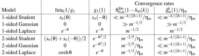
Convergence rates
Model lim01/g1 g1(1) πˆSto0,m(1−hm(k)) gˆkm(1)/ηm
1-sided Student sν(θ) sν(−θ) ≪m−k/(2k+1)/ηm ≪m−k/(2k+1)/ηm
1-sided Gaussian 0 0 ≫m−1/3 ≫m−1/3
1-sided Laplace e−θ e−θ m−1/2 m−1/2
2-sided Student (sν(θ) +sν(−θ))/2 e−θ
2/2
m−2/5/ηm ≪m−k/(2k+1)/ηm
2-sided Gaussian 0 e−θ2/2 m−2/5/ηm ≪m−k/(2k+1)/ηm
2-sided Laplace coshθ e−θ m−1/3/η
m ≪m−k/(2k+1)/ηm Table 2: Properties of one- and two-sided test statistics distributions in Student, Gaussian, and
Laplace models, and convergence rates of the kernel estimators studied. When the rate depends onk, the value ofkmay be chosen arbitrarily large. ηm is a sequence such that ηm→0 andmηm→+∞asm→+∞.
π0+ (1−π0)e−θ 2/2
at ratem−2/5, by Corollary 17. Conversely, the density of one-sided p-values tends to 0 at 1, but is not differentiable: the trueπ0can be estimated consistently, but the convergence
rate is slower.
6. Concluding Remarks
This paper studies asymptotic properties of a family of plug-in procedures based on the BH pro-cedure. When compared to the BH procedure or to the Storey-λprocedure, the results for general models obtained in Section 4 show that incorporating the proposed estimators ofπ0into the BH
pro-cedure asymptotically yields (i) tighter FDR control (or, equivalently, greater power) and (ii) smaller critical values, thereby increasing the range of situations in which the resulting procedure has pos-itive asymptotic power. These improvements come at the price of a reduction in the convergence rate from the parametric ratem−1/2to a non-parametric ratem−k/(2k+1), wherekis connected to the order of differentiability of the test statistics distribution. As the results obtained for the proposed modification of the Storey-λestimator ˆπSto
0,m(1−hm)require stronger conditions (null derivatives of
g1) than for kernel estimators with a kernel of orderk, we conclude that it is generally better to use
the latter class of estimators.
Our application of these results to specific models for the test statistics sheds some light on the influence of the test statistics distribution on convergence rates of plug-in procedures:
• When the test statistics distribution isC∞(which is the case for two-sided Gaussian test statis-tics, and for Laplace and Student tests statistics), the obtained convergence rates are slower than the parametric rate, but may be arbitrarily close to it by choosing a kernel of sufficiently high order. The resulting estimators are not consistent estimators of π0, although the bias
decreases as the non-centrality parameterθincreases.
N
(0,1)vsN
(1,1)Figure 4: Density of one- and two-sidedp-values under the alternative hypothesis for the location model
N
(0,1)versusN
(1,1). Inserted plot: zoom in the region[0.9,1], which is high-lighted by a black box in the main plot.Obtaining more precise conclusions in the context of a specific data set or application exceeds the scope of the present paper, as it would require extending the obtained results to more realistic settings such as the ones that are now described.
6.1 Extensions of the Multiple Testing Setting Considered
in Chi (2007a) essentially relies on the assumption that the p-values are independently and identi-cally distributed. Therefore, it seems that these results could be extended to composite distributions under
H
1, provided that the corresponding marginal distributions are still independently and identi-cally distributed. Extending these results to settings where the independence assumption is relaxed seems a more challenging question. As for the convergence results established in Section 4, their proofs rely on the formalism laid down by Neuvial (2008). Therefore, these results could be ex-tended to other dependency assumptions, or to composite distributions underH
1provided that the convergence in distribution of the empirical distribution functions (Gb0,m,Gb1,m) holds under theseassumptions. In that spirit, the results of Neuvial (2008) have been extended to an equi-correlated Gaussian model (Delattre and Roquain, 2011) and to a more general Gaussian model where the covariance matrix is supposed to be close enough to the identity as the number of tests grows to infinity (Delattre and Roquain, 2012).
Second, we have shown that the asymptotic properties of FDR controlling procedures are driven by the shape and regularity of the test statistics distribution. In practice, the test statistics distribu-tion depends on the size of the sample used to generate them. In differential expression analyses, a natural test statistic is Student’st, whose distribution depends on sample size through both the number of degrees of freedomνand a non-centrality parameterθ. In the spirit of the results of Chi (2007b) on the influence of sample size on criticality, it would be interesting to study the conver-gence rates of plug-in procedures when both the sample size and the number of hypotheses tested grow to infinity.
6.2 Alternative Strategies to Estimateπ0
The estimators ofπ0considered in this paper are kernel estimators of the densitygat 1. Therefore,
they achieve non-parametric convergence rates of the form m−k/(2k+1)/ηm, where k controls the regularity ofg near 1 andηm→0 slowly enough. An interesting open question is whether these non-parametric rates may be improved. Other strategies for estimatingπ0 may be considered to
achieve faster convergence rates, including the following two:
• One-stage adaptive procedures as proposed by Blanchard and Roquain (2009) and Finner et al. (2009) allow more powerful FDR control than the standard BH procedure without ex-plicitly incorporating an estimate ofπ0: they are not plug-in procedures.
• Jin (2008) proposed an estimator ofπ0 based on the Fourier transform of the empirical
char-acteristic function of theZ-scores associated to thep-values. This estimator does not focus on the behavior of the density near 1, and might not suffer from the same limitations as the esti-mators studied here. This estimator was shown to be consistent for the estimation ofπ0when
theZ-scores follow a Gaussian location mixture, but no convergence rates were established.
In a general semi-parametric framework whereg1 is not necessarily decreasing, and its regularity is not specified, Nguyen and Matias (2013) have recently proved that if the Lebesgue measure of the set on whichg1achieves its minimum is null, then no consistent estimator of mintg(t) with a finite asymptotic variance can reach the parametric convergence ratem−1/2. In our setting where
g1 is decreasing, the measure of the set on whichg1 is minimum is indeed null, except if g1 is
constant on an interval of the form[t0,1]. For one-sided tests whereg1(t) = (f1/f0)(F0−1(1−t)),
this extreme situation arises if and only if the likelihood ratio is constant on an interval of the form
Laplace model, where(f1/f0)(x) =exp(|x| − |x−θ|) =eθforx≥θ>0. The kernel estimators that
we have studied here do reach the ratem−1/2in this case.
In the more common situation in which the measure of the set on whichg1vanishes (or achieves
its minimum) is null, the above negative result of Nguyen and Matias (2013) suggests that there is little room for improving on the non-parametric convergence rates obtained in Propositions 14 and 15. We conjecture that it is not possible for consistent estimators ofg(1)to reach a parametric convergence rate in this setting.
Acknowledgments
The author would like to thank Stéphane Boucheron for insightful advice and comments, and Catherine Matias and Etienne Roquain for many useful discussions. He is also grateful to anony-mous referees for very constructive comments and suggestions that greatly helped improve the pa-per.
This work was partly supported by the association “Courir pour la vie, courir pour Curie”, and by the French ANR project TAMIS.
Appendix A. Calculations in Specific Models
In this section we perform calculations in location and Student models.
A.1 Location Models
Lemma 22 gives the distribution of the p-value under the alternative hypothesis for one-sided tests in the Laplace model. The proof is straightforward, so it is omitted.
Lemma 22 (One-sided Laplace location model) Assume that the probability distribution function
of the test statistics is f0 :x7→ 12e−|x| under the null hypothesis, and f1:x7→ 12e−|x−θ| under the alternative, withθ>0(one-sided test). Then
1. The one-sidedp-value function is
1−F0(x) =
(
1 2e(−|
x|) if x≥0
1−12e(−|x|) if x<0 ;
2. The inverse one-sidedp-value function is
(1−F0)−1(t) =
(
ln 21t if0≤t≤12 ln(2(1−t)) if 1
2<t<1
;
3. The cdf of one-sidedp-values under
H
1isG1(t) =
teθ if0≤t≤e−θ
2
1−41te−θ if e−2θ ≤t≤12 1−(1−t)e−θ if t≥1
2
4. The probability distribution function of one-sidedp-values under
H
1isg1(t) =
eθ if0≤t≤e−θ
2 1
4t2e−θ if e
−θ
2 ≤t≤ 1 2 e−θ if t≥1
2
.
Proposition 23 (Concavity in two-sidedγ-Subbotin models) If the test statistics follow aγ-Subbotin distribution withγ∈[1,2], then the distribution function of the two-sided p-values under the alter-native G1is concave.
Proof [Proof of Proposition 23] Assumption (1) holds for Subbotin models. By Lemma 2, we need to prove that the likelihood ratio f1γ/f0γ of theγ-Subbotin model with γis such thath:x7→
(f1γ/f0γ)(x) + (f1γ/f0γ)(−x)is non-decreasing onR+. The functionhis differentiable on(0,+∞)\
{θ}, and its derivative is given by
h′(x) =
fγ
1 f0γ
′
(x)−
fγ
1 f0γ
′
(−x),
where
fγ
1 f0γ
′
(y) =sgn(y)|y|γ−1
−sgn(y−θ)|y−θ|γ−1 f
γ
1
f0γ(y) (15)
for anyy∈R\ {0,θ}. Letx>0 such thatx6=θ, we are going to prove thath′(x)≥0. As fγ
1/f
γ
0 is
non-decreasing, both f1γ/f0γ′(x)and f1γ/f0γ′(−x) are non-negative. If f1γ/f0γ′(−x) =0, then
h′(x)≥0 as desired. From now on, we assume that fγ
1/f
γ
0
′
(−x)is positive. Asθ>0, (15) entails that
f1γ/f0γ′(x)
f1γ/f0γ′(−x) =
xγ−1−sgn(x−θ)|x−θ|γ−1
(x+θ)γ−1−xγ−1
f1(x)γ f1(−x)γ
,
where f1(x)γ> f1(−x)γbecause−|x−θ|+|x+θ|>0. As f1γ/f
γ
0
′(
−x)>0, it is enough to show that
xγ−1
−sgn(x−θ)|x−θ|γ−1≥(x+θ)γ−1−xγ−1 (16)
in order to prove that h′(x)≥0. By the concavity of x7→ xγ−1 on R+ for 1≤γ≤2, φ:x 7→
θ−1(xγ−1−(x−θ)γ−1)is non-increasing on [θ,+∞]. Therefore, ifx>θwe haveφ(x)≥φ(x+θ)
and (16) holds. Ifx<θ, then noting that for anya,b>0 andζ∈[0,1],aζ+bζ≥(a+b)ζ, we have, for 1≤γ≤2,xγ−1+ (θ−x)γ−1≥θγ−1≥(x+θ)γ−1
−xγ−1, and (16) holds as well.
A.2 Student Model