Dynamic Policy Programming
Mohammad Gheshlaghi Azar [email protected]
Vicenc¸ G´omez [email protected]
Hilbert J. Kappen [email protected]
Department of Biophysics Radboud University Nijmegen 6525 EZ Nijmegen, The Netherlands
Editor:Ronald Parr
Abstract
In this paper, we propose a novel policy iteration method, called dynamic policy programming (DPP), to estimate the optimal policy in the infinite-horizon Markov decision processes. DPP is an incremental algorithm that forces a gradual change in policy update. This allows us to prove finite-iteration and asymptotic ℓ∞-norm performance-loss bounds in the presence of approxima-tion/estimation error which depend on the average accumulated error as opposed to the standard bounds which are expressed in terms of the supremum of the errors. The dependency on the av-erage error is important in problems with limited number of samples per iteration, for which the average of the errors can be significantly smaller in size than the supremum of the errors. Based on these theoretical results, we prove that a sampling-based variant of DPP (DPP-RL) asymptotically converges to the optimal policy. Finally, we illustrate numerically the applicability of these results on some benchmark problems and compare the performance of the approximate variants of DPP with some existing reinforcement learning (RL) methods.
Keywords: approximate dynamic programming, reinforcement learning, Markov decision pro-cesses, Monte-Carlo methods, function approximation
1. Introduction
ADP methods have been successfully applied to many real world problems, and theoretical results have been derived in the form of finite iteration and asymptotic performance guarantee on the induced policy. In particular, the formal analysis of these algorithms is usually characterized in terms of bounds on the difference between the optimal and the estimated value function induced by the algorithm (performance loss) (Farahmand et al., 2010; Thiery and Scherrer, 2010; Munos, 2005; Bertsekas and Tsitsiklis, 1996). For instance, in the case of AVI and API, the asymptoticℓ∞-norm performance-loss bounds in the presence of approximation errorεkcan be expressed as1
lim sup
k→∞ k
Q∗−Qπkk ≤ 2γ
(1−γ)2lim sup
k→∞ k
εkk, (1)
whereγdenotes the discount factor, k · kis theℓ∞-norm w.r.t. the state-action pair(x,a)andπk is
the control policy at iterationk.
The bound of Equation 1 is expressed in terms of the supremum of the approximation errors. Intuitively, the dependency on the supremum error means that to have a small overall performance loss the approximation errors of all iterations should be small in size, that is, a large approximation error in only one iteration can derail the whole learning process. This can cause a major problem when the approximation errorεk arises from sampling. In many problems of interest, the sampling
error can be large and hard to control, since only a limited number of samples can be used at each iteration. Also, even in those cases where we have access to large number of samples, it may be difficult, if not impossible, to control the size of errors for all iterations. This is due to the fact that the sampling errors are random objects and, regardless of the number of samples used at each iteration, there is always a fair chance that in some fewoutlieriterations the sampling errors take large values in their interval of definition. In all those cases, a bound which depends on the average accumulated error ¯εk=1/(k+1)∑kj=0εjinstead of the supremum error is preferable. The rationale
behind this idea is that the average of the sum of random variables, under some mild assumptions, can be significantly smaller in size than the supremum of the random variables. Also, the average error ¯εkis less sensitive to the outliers than the supremum error. Therefore, a bound which depends
on the average error can be tighter than the one with dependency on the supremum error. To the best of authors’ knowledge, there exists no previous work that provides such a bound.
In this paper, we propose a new incremental policy-iteration algorithm called dynamic policy programming (DPP). DPP addresses the above problem by proving the first asymptotic and finite-iteration performance loss bounds with dependency onkε¯kk. This implies the previously mentioned advantages in terms of performance guarantees. The intuition is that DPP, by forcing an incremental change between two consecutive policies, accumulates the approximation errors of all the previous iterations, rather than just minimizing the approximation error of the current iteration. We also introduce a new RL algorithm based on the DPP update rule, called DPP-RL, and prove that it converges to the optimal policy with the convergence rate of order 1/√k. This rate of convergence leads to a PAC (“probably approximately correct”) sample-complexity bound of orderO(1/((1− γ)6ε2))to find anε-optimal policy with high probability, which is superior to the best existing result of standard Q-learning (Even-Dar and Mansour, 2003). See Section 6 for a detailed comparison with incremental RL algorithms such as Q-learning and SARSA.
1. For AVI the approximation errorεkis defined as the error associated with the approximation of the Bellman optimality
operator. In the case of API,εkis the policy evaluation error (see Farahmand et al., 2010; Bertsekas and Tsitsiklis,
DPP shares some similarities with the well-known actor-critic (AC) method of Barto et al. (1983), since both methods make use of an approximation of the optimal policy by means of action preferences and soft-max policy. However, DPP uses a different update rule which is only expressed in terms of the action preferences and does not rely on the estimate of the value function to criticize the control policy.
The contribution of this work is mainly theoretical, and focused on the problem of estimating the optimal policy in an infinite-horizon MDP. Our setting differs from the standard RL setting in the following: we rely on agenerative model from which samples can be drawn. This means that the agent has full control on the sample queries that can be made for any arbitrary state. Such an assumption is commonly made in theoretical studies of RL algorithms (Farahmand et al., 2008; Munos and Szepesv´ari, 2008; Kearns and Singh, 1999) because it simplifies the analysis of learning and exploration to a great extent. We compare DPP empirically with other methods that make use of this assumption. The reader should notice that this premise does not mean that the agent needs explicit knowledge of the model dynamics to perform the required updates, nor does it need to learn one.
This article is organized as follows. In Section 2, we present the notation which is used in this paper. We introduce DPP and we investigate its convergence properties in Section 3. In Section 4, we demonstrate the compatibility of our method with the approximation techniques by generalizing DPP bounds to the case of function approximation and Monte-Carlo sampling. We also introduce a new convergent RL algorithm, called DPP-RL, which relies on a sampling-based variant of DPP to estimate the optimal policy. Section 5, presents numerical experiments on several problem domains including the optimal replacement problem (Munos and Szepesv´ari, 2008) and a stochastic grid world. In Section 6 we briefly review some related work. Finally, in Section 7, we summarize our results and discuss some of the implications of our work.
2. Preliminaries
In this section, we introduce some concepts and definitions from the theory of Markov decision pro-cesses (MDPs) and reinforcement learning (RL) as well as some standard notation (see Szepesv´ari, 2010, for further reading). We begin by the definition of theℓ2-norm (Euclidean norm) and the
ℓ∞-norm (supremum norm). Assume thatYis a finite set. Given the probability measureµoverY, for a real-valued functiong:Y→R, we shall denote theℓ2-norm and the weightedℓ2,µ-norm ofg
bykgk22,∑y∈Yg(y)2andkgk22,µ,∑y∈Yµ(y)g(y)2, respectively. Also, theℓ∞-norm ofgis defined bykgk,maxy∈Y|g(y)|and log(·)denotes the natural logarithm.
2.1 Markov Decision Processes
A discounted MDP is a quintuple(X,A,P,R,γ), whereXandAare, respectively, the state space and the action space.Pshall denote the state transition distribution andRdenotes the reward kernel. γ∈[0,1)denotes the discount factor. The transitionPis a probability kernel over the next state upon taking actionafrom statex, which we shall denote byP(·|x,a). Ris a set of real-valued numbers. A rewardr(x,a)∈Ris associated with each statexand actiona.
Remark 1 To keep the representation succinct, we make use of the short-hand notationZfor the joint state-action spaceX×A. We also denote Rmax
(1−γ)by Vmax.
A Markovian policy kernel determines the distribution of the control action given the current state. The policy is called stationary if the distribution of the control action is independent of time. Given the current statex, we shall denote the Markovian stationary policy, or in short only policy, byπ(·|x). A policy is called deterministic if for any statex∈Xthere exists some actionasuch that π(a|x) =1. Given the policyπ, its corresponding value functionVπ:X→Rdenotes the expected total discounted reward in each statex, when the action is chosen by policyπ, which we denote by
Vπ(x). Often it is convenient to associate value functions not with states but with state-action pairs. Therefore, we introduceQπ:Z→Ras the expected total discounted reward upon choosing actiona
from statexand then following policyπ, which we shall denote byQπ(x,a). We define theBellman operatorTπon the action-value functions by2
TπQ(x,a),r(x,a) +γ
∑
(y,b)∈Z
P(y|x,a)π(b|y)Q(y,b), ∀(x,a)∈Z.
The goal is to find a policyπ∗that attains theoptimal value function,V∗(x),supπVπ(x), at all statesx∈X. The optimal value function satisfies the Bellman equation:
V∗(x) = sup π(·|x)y
∑
∈Xa∈A
π(a|x) [r(x,a) +P(y|x,a)V∗(y)]
=max
a∈A
"
r(x,a) +
∑
y∈X
P(y|x,a)V∗(y) #
,
∀x∈X. (2)
Likewise, the optimal action-value function Q∗ is defined by Q∗(x,a) =supπQπ(x,a) for all (x,a)∈Z. We shall define theBellman optimality operatorTon the action-value functions as
TQ(x,a),r(x,a) +γ
∑
y∈X
P(y|x,a)max
b∈AQ(y,b), ∀(x,a)∈Z.
Q∗is the fixed point ofT. BothTandTπare contraction mappings, w.r.t. the supremum norm, with the factorγ(Bertsekas, 2007, Chapter 1). In other words, for any two real-valued action-value functionsQandQ′ and every policyπ, we have
TQ−TQ′≤γQ−Q′, TπQ−TπQ′≤γQ−Q′.
The policy distributionπdefines a right-linear operatorPπ·as
(PπQ)(x,a),
∑
(y,b)∈Z
π(b|y)P(y|x,a)Q(y,b), ∀(x,a)∈Z.
Further, we define two other right-linear operatorsπ·andP·as
(πQ)(x),
∑
a∈A
π(a|x)Q(x,a), ∀x∈X,
(PV)(x,a),
∑
y∈X
P(y|x,a)V(y), ∀(x,a)∈Z.
We note that for everyQ:Z→R,V :X→Rand policyπ, we have
(π[Q+V])(x) = (πQ)(x) +V(x), ∀x∈X,
(Pπ[Q+V])(x,a) = (PπQ)(x,a) + (PV)(x,a), ∀(x,a)∈Z. (3)
We define the max operatorMon the action value functions as(MQ)(x),
maxa∈AQ(x,a), for allx∈X. Based on the new definitions one can rephrase the Bellman operator
and the Bellman optimality operator as
TπQ(x,a) =r(x,a) +γ(PπQ)(x,a), TQ(x,a) =r(x,a) +γ(PMQ)(x,a).
In the sequel, we repress the state(-action) dependencies in our notation wherever these depen-dencies are clear, for example,Ψ(x,a)becomesΨ,Q(x,a)becomesQ. Also, for simplicity of the notation, we remove some parenthesis, for example, writingMQ for(MQ)and PπQfor (PπQ), when there is no possible confusion.
3. Dynamic Policy Programming
In this section, we introduce and analyze the DPP algorithm. We first present thedynamic policy programming (DPP) algorithm in Section 3.1 (see Appendix A for some intuition on how DPP can be related to the Bellman equation). We then investigate the finite-iteration and the asymptotic behavior of DPP and prove its convergence in Section 3.2.
3.1 Algorithm
DPP is a policy iteration algorithm which represents the policyπk in terms of some action
prefer-ence numbersΨk (Sutton and Barto, 1998, Chapter 2.8). Starting at Ψ0, DPP iterates the action
preferences of all state-action pairs(x,a)∈Zthrough the DPP operatorO(the pseudo code of DPP is presented in Algorithm 1):
Ψk+1(x,a) =OΨk(x,a),Ψk(x,a)−(MηΨk)(x) +r(x,a) +γ(PMηΨk)(x,a),
whereMηdenotes the softmax operator. The softmax operatorMη is defined on every f :Z→R as
(Mηf)(x), ∑
a∈A
exp(ηf(x,a))f(x,a)
∑
b∈A
exp(ηf(x,b)) ,
whereη>0 is the inverse temperature.
The control policyπkis then computed as a function ofΨkat each iterationk:
πk(a|x) =
exp(ηΨk(x,a))
∑
b∈A
exp(ηΨk(x,b))
, ∀(x,a)∈Z. (4)
Ψk+1(x,a) =Ψk(x,a) +TπkΨk(x,a)−πkΨk(x), ∀(x,a)∈Z. (5)
Algorithm 1:(DPP) Dynamic Policy Programming Input: Action preferencesΨ0(·,·),γandη
1 fork=0,1,2, . . . ,K−1do // main loop
2 foreach (x,a)∈Zdo // compute the control policy
3 πk(a|x):= exp(ηΨk(x,a))
∑
b∈A
exp(ηΨk(x,b))
;
4 end
5 foreach (x,a)∈Zdo // compute the new action-preferences
6 Ψk+1(x,a):=Ψk(x,a) +TπkΨ
k(x,a)−πkΨk(x); // DPP update rule
7 end
8 end
9 foreach (x,a)∈Zdo // compute the last policy
10 πK(a|x):= exp(ηΨK(x,a))
∑
b∈A
exp(ηΨK(x,b))
;
11 end 12 returnπK;
3.2 Performance Guarantee
In this subsection, we investigate the finite-iteration and asymptotic behavior of Algorithm 1. We begin by proving a finite-iteration performance guarantee for DPP:
Theorem 2 ( Theℓ∞-norm performance loss bound of DPP) Let Assumption 1 hold. Also,
as-sume thatΨ0is uniformly bounded by Vmaxfor all(x,a)∈Z, then the following inequality holds for
the policy induced by DPP at iteration k≥0:
kQ∗−Qπkk ≤
2γ4Vmax+log(|
A|)
η
(1−γ)2(k+1) . Proof See Appendix B.1.
Note that the DPP algorithm converges to the optimal policy for every η>0 and choosing a differentη only changes the rate of convergence. The best rate of convergence is achieved by settingη=∞, for which the softmax policy and the softmax operatorMη are replaced with the greedy policy and the max-operatorM, respectively. Therefore, forη= +∞the DPP recursion is re-expressed as
We must point out that the choice ofη<+∞may be still useful in the presence of function approximation, where the greedy update rule can be unstable due to the non-differentiability of the max operator. In fact, our numerical results in Section 5.2 suggests that the performance of DPP in the presence of function approximation is optimized for some finite value ofηrather thanη= +∞ (see Section 5.2 for more details).
As an immediate consequence of Theorem 2, we obtain the following result:
Corollary 3 The following relation holds in limit:
lim
k→+∞Q
πk(x,a) =Q∗(x,a), ∀(x,a)∈Z.
In words, the policy induced by DPP asymptotically converges to the optimal policyπ∗. The following corollary shows that there exists a unique limit for the action preferences in infinity if the optimal policyπ∗is unique.
Corollary 4 Let Assumption 1 hold and k be a non-negative integer. Assume that the optimal policy
π∗ is unique and letΨk(x,a), for all(x,a)∈Z, be the action preference after k iteration of DPP.
Then, we have:
lim
k→+∞Ψk(x,a) =
V∗(x) a=a∗(x)
−∞ otherwise , ∀x∈X.
Proof See Appendix B.2.
Notice that the assumption on the uniquenessof the optimal policyπ∗ is not required for the main result of this section (Theorem 2). Also, the fact that in Corollary 4 the action preferences of sub-optimal actions tend to−∞is the natural consequence of the convergence ofπkto the optimal
policyπ∗, which forces the probability of the sub-optimal actions to be 0.
4. Dynamic Policy Programming with Approximation
Algorithm 1 (DPP) only applies to small problems with a few states and actions. Also, to compute the optimal policy by DPP an explicit knowledge of the model is required. In many real world problems, this information is not available. Instead it may be possible to simulate the state tran-sition by Monte-Carlo sampling and thenestimatethe optimal policy using these samples. In this section, we first prove some general bounds on the performance of DPP in the presence of approxi-mation/estimation error and compare these bounds with those of AVI and API. We then present new approximate algorithms for implementing DPP with Monte-Carlo sampling (DPP-RL) and linear function approximation (SADPP). For both DPP-RL and SADPP we assume that we have access to the generative model of MDP, that is, an oracle can generate the next sampleyfromP(·|x,a)for every state-action pair(x,a)∈Zon the request of the learner.
4.1 Theℓ∞-Norm Performance-Loss Bounds for Approximate DPP
εk(x,a),Ψk+1(x,a)−OΨk(x,a), ∀(x,a)∈Z. (6)
Note that this definition ofεkis rather general and does not specify the approximation technique
used to compute Ψk+1. In the following subsections, we provide specific update rules to
approx-imateΨk+1 for both DPP-RL and SADPP algorithms which also makes the definition ofεk more
specific.
The approximate DPP update rule then takes the following forms:
Ψk+1(x,a) =OΨk(x,a) +εk(x,a)
=Ψk(x,a) +r(x,a) +γPMηΨk(x,a)−MηΨk(x,a) +εk(x,a)
=Ψk(x,a) +TπkΨk(x,a)−πkΨk(x,a) +εk(x,a),
(7)
whereπkis given by Equation 4.
We begin by the finite-iteration analysis of approximate DPP. The following theorem establishes an upper-bound on the performance loss of DPP in the presence of approximation error. The proof is based on generalization of the bound that we established for DPP by taking into account the error εk:
Theorem 5 (Finite-iteration performance loss bound of approximate DPP) Let Assumption 1 hold. Assume that k is a non-negative integer andΨ0is bounded by Vmax. Further, defineεk for all k by Equation 6 and the accumulated error Ekas
Ek(x,a),
k
∑
j=0
εj(x,a), ∀(x,a)∈Z.
Then the following inequality holds for the policy induced by approximate DPP at round k:
kQ∗−Qπkk ≤ 1
(1−γ)(k+1) 2γ
4Vmax+log(|
A|)
η
(1−γ) +
k
∑
j=0 γk−jkE
jk
.
Proof See Appendix C.
Taking the upper-limit yields corollary 6.
Corollary 6 (Asymptotic performance-loss bound of approximate DPP) Define
¯
ε,lim supk→∞kEkk
(k+1). Then, the following inequality holds:
lim sup
k→∞ k
Q∗−Qπkk ≤ 2γ
(1−γ)2ε¯. (8)
The asymptotic bound is similar to the existing results of AVI and API (Thiery and Scherrer, 2010; Bertsekas and Tsitsiklis, 1996, Chapter 6):
lim sup
k→∞ k
Q∗−Qπkk ≤ 2γ
whereεmax=lim supk→∞kεkk. The difference is that in Equation 8 the supremum norm of error
εmaxis replaced by the supremum norm of the average error ¯ε. In other words, unlike AVI and API, the size of error at each iteration is not a critical factor for the performance of DPP and as long as the size of average error remains close to 0, DPP is guaranteed to achieve a near-optimal performance even when the individual errorsεk are large
As anexample: Consider a case in which, for both DPP and AVI/API, the sequence of errors
{ε0,ε1,ε2, . . .} are some i.i.d. zero-mean random variables bounded by 0<U <∞. Corollary 6 combined with the law of large numbers then leads to the following asymptotic bound for approxi-mate DPP:
lim sup
k→∞ k
Q∗−Qπkk ≤ 2γ
(1−γ)2ε¯=0, w.p. (with probability) 1, whilst for API and AVI we have
lim sup
k→∞ k
Q∗−Qπkk ≤ 2γ
(1−γ)2U.
In words, approximate DPP manages to cancel i.i.d. noise and asymptotically converges to the optimal policy whereas there is no guarantee, in this case, for the convergence of API and AVI to the optimal solution. This example suggests that DPP, in general, may average out some of the simulation noise caused by Monte-Carlo sampling and eventually achieve a better performance than AVI and API in the presence of sampling error.
Remark 7 The i.i.d. assumption may be replaced by some weaker and more realistic assumption that only requires the error sequence{ε0,ε1, . . . ,εk}to be a sequence of martingale differences, that is, the errors do not need to be independent as long as the expected value ofεk, conditioned on the past observations, is0. We prove, in the next subsection, that DPP-RL satisfies this assumption and, therefore, asymptotically converges to the optimal policy (see Theorem 9).
4.2 Reinforcement Learning with Dynamic Policy Programming
To compute the optimal policy by DPP one needs an explicit knowledge of the model. In many prob-lems, we do not have access to this information but instead we can generate samples by simulating the model. The optimal policy can then belearnedusing these samples. In this section, we introduce a new RL algorithm, called DPP-RL, which relies on a sampling-based variant of DPP to update the policy. The update rule of DPP-RL is very similar to Equation 5. The only difference is that we replace the Bellman operatorTπΨ(x,a)with its sample estimateTπkΨ(x,a),r(x,a) +γ(πΨ)(yk), where the next sampleykis drawn fromP(·|x,a):
Ψk+1(x,a),Ψk(x,a) +TkπkΨk(x,a)−πkΨk(x), ∀(x,a)∈Z. (9)
Based on Equation 9, we estimate the optimal policy by iterating some initialΨ0 through the DPP-RL update rule, where at each iteration we drawyk for every(x,a)∈Z. From Equation 6, the estimation error of thekth iterate of DPP-RL is then defined as the difference between the Bellman operatorTπkΨ
k(x,a)and its sample estimate:
The DPP-RL update rule can then be considered as a special case of the more general approxi-mate DPP update rule of Equation 7.
Equation 9 is just an approximation of the DPP update rule of Equation 5. Therefore, the convergence result of Corollary 3 does not hold for DPP-RL. However, the new algorithm still converges to the optimal policy since one can show that the errors associated with approximating Equation 5 are asymptoticallyaveraged outby DPP-RL, as postulated by Corollary 6. To prove this result we need the following lemma, which bounds the estimation errorεk.
Lemma 8 (Boundedness ofεk) Let Assumption 1 hold and assume that the initial action-preference functionΨ0is uniformly bounded by Vmax, then we have, for all k≥0,
Tπk
k Ψk
≤2γlog(|A|)
η(1−γ) +Vmax, kεkk ≤
4γlog(|A|)
η(1−γ) +2Vmax. Proof See Appendix D.
Lemma 8 is an interesting result, which shows that, despite the fact that Ψk tends to−∞for
the sub-optimal actions, the error εk is uniformly bounded by some finite constant. Note that
εk=TπkΨk−TkπkΨkcan be expressed in terms of the soft-maxMηΨk, which unlikeΨk, is always
bounded by a finite constant, for everyη>0.
The following theorem establishes the asymptotic convergence of DPP-RL to the optimal policy.
Theorem 9 (Asymptotic convergence of DPP-RL) Let Assumption 1 hold. Assume that the initial action-value functionΨ0is uniformly bounded by Vmaxandπk is the policy induced byΨk after k iteration of DPP-RL. Then, w.p. 1, the following holds:
lim
k→∞Q
πk(x,a) =Q∗(x,a), ∀(x,a)∈Z.
Proof See Appendix D.1.
We also prove the following result on the converge rate of DPP-RL to the optimal policy by making use of the result of Theorem 5:
Theorem 10 (Finite-time high-probability loss-bound of DPP-RL) Let Assumption 1 hold and k be a positive integer and0<δ<1. Then, at iteration k of DPP-RL with probability at least1−δ, we have
kQ∗−Qπkk ≤ 4(γlog(|A|)/η+2Rmax)
(1−γ)3
1
k+1+ s
2 log2|Xδ||A|
k+1
.
Proof See Appendix D.2.
Theorem 5 implies that, regardless of the value ofηandγ, DPP-RL always converges with the rate of 1/√k.
Corollary 11 Let Assumption 1 hold and k be a positive integer, also set the inverse temperature
η= +∞, Then, at iteration k of DPP-RL with probability at least1−δ, we have
kQ∗−Qπkk ≤ 8Rmax
(1−γ)3 1
k+1+ s
2 log2|Xδ||A|
k+1 .
This result implies that, in order to achieve the best rate of convergence, one can set the value ofηto+∞, that is, to replace the soft-maxMηwith the max operatorM:
Ψk+1(x,a):=Ψk(x,a) +TkΨk(x,a)−MΨk(x), ∀(x,a)∈Z,
whereTkΨ(x,a),r(x,a) +γ(MΨ)(yk)for all(x,a)∈Z. The pseudo-code of DPP-RL algorithm, which setsη= +∞, is shown in Algorithm 2.
Algorithm 2:(DPP-RL) Reinforcement learning with DPP
Input: Initial action preferencesΨ0(·,·), discount factorγand number of stepsT
1 fork=1,2,3, . . . ,K−1do // main loop
2 foreach (x,a)∈Zdo // update Ψk(·,·) for all state-action pairs
3 yk∼P(·|x,a); // generate the next sample
4 TkΨk(x,a):=r(x,a) +γMΨk(yk); // empirical Bellman operator
5 Ψk+1(x,a):=Ψk(x,a) +TkΨk(x,a)−MΨk(x); // DPP update rule
6 end
7 foreach x∈Xdo // compute the control policy
8 amax:=arg maxa∈AΨk+1(x,a);
9 π(·|x):=0;
10 πk+1(amax|x):=1; 11 end
12 end 13 returnπK
Furthermore, the following PAC bound which determines the number of steps k required to achieve the errorε>0 in estimating the optimal policy, w.p. 1−δ, is an immediate consequence of Theorem 10.
Corollary 12 (Finite-time PAC bound of DPP-RL) Let Assumption 1 hold. Then, for anyε>0, after
k=256R 2 maxlog
2|X||A|
δ (1−γ)6ε2 .
steps of Algorithm 2, the uniform approximation errorkQ∗−Qπkk ≤ε, w. p. 1−δ.
a set of basis functionsFφ={φ1, . . . ,φm}, where eachφi:Z→Ris a bounded real valued function,
the sequence of action preferences {Ψ0,Ψ1,Ψ2. . .} are defined as a linear combination of these basis functions:Ψk=θTkΦ, whereΦis am×1 column vector with the entries{φi}i=1:mandθk∈Rm
is am×1 vector of parameters.
The action preference functionΨk+1is an approximation of the DPP operatorOΨk. In the case
of LFA the common approach to approximate DPP operator is to find a vectorθk+1 that projects OΨkon the column space spanned byΦby minimizing the loss function:
Jk(θ;Ψ),
θTΦ−OΨ
k
2 2,µ,
whereµis a probability measure on Z. The best solution, which minimizes J, is called the least-squares solution:
θk+1=arg min
θ∈RmJk(θ;Ψ) =
E ΦΦT−1E(ΦOΨk),
where the expectation is taken w.r.t. (x,a)∼µ. In principle, to compute the least squares solution equation one needs to computeOΨkfor all states and actions. For large scale problems this becomes
infeasible. Instead, one can make a sample estimate of the least-squares solution by minimizing the empirical lossJek(θ;Ψ)(Bertsekas, 2007, Chapter 6.3):
e
Jk(θ;Ψ), 1
N N
∑
n=1
(θTΦ(Xn,An)−OnΨk)2+αθTθ,
where{(Xn,An)}n=1:Nis a set ofNi.i.d. samples drawn from the distributionµ. Also,OnΨkdenotes
a single sample estimate ofOΨk(Xn,An)defined byOnΨk,Ψk(Xn,An) +r(Xn,An) +γMηΨk(Yn)−
MηΨk(Xn), whereYn∼P(·|Xn,An). Further, to avoid over-fitting due to the small number of
sam-ples, one adds a quadratic regularization term to the loss function. The empirical least-squares solution which minimizesJke(θ;Ψ)is given by
e θk+1=
"
N
∑
n=1
Φ(Xn,An)Φ(Xn,An)T+αNI
#−1
N
∑
n=1
OnΨkΦ(Xn,An), (10)
andΨk(x,a) =eθk+1Φ(x,a). This defines a sequence of action preferences{Ψ0,Ψ1,Ψ2, . . .}and the sequence of approximation error through Equation 6.
Algorithm 3 presents thesampling-based approximate dynamic policy programming(SADPP) in which we rely on Equation 10 to approximate DPP operator at each iteration.
5. Numerical Results
In this section, we illustrate empirically the theoretical performance guarantee introduced in the previous sections for both variants of DPP: the exact case (DPP-RL) and the approximate case (SADPP). In addition, we compare with existing algorithms for which similar theoretical results have been derived.
Algorithm 3:(SADPP) Sampling-based approximate dynamic policy programming Input:eθ0,η,γ,α,KandN
1 fork=0,1,2, . . . ,K−1do // main loop
2 {(Xn,An)}n=1:N∼µ(·,·); // generate n i.i.d. samples from µ(·,·)
3 {Yn}n=1:N∼P(·|{(Xn,An)}n=1:N); // generate next states from P(·|·) 4 foreachn=1,2,3, . . . ,Ndo
5 foreach a∈Ado // compute Ψk for every action of states Xn,Yn 6 Ψk(Xn,a) =eθT
kΦ(Xn,a); 7 Ψk(Yn,a) =eθTkΦ(Yn,a);
8 end
9 MηΨk(Xn) = ∑
a∈A
exp(ηΨk(Xn,a))Ψk(Xn,a)
∑
b∈A
expηΨk(Xn,b) ;
10 MηΨk(Yn) = ∑ a∈A
exp(ηΨk(Yn,a))Ψk(Yn,a)
∑
b∈A
expηΨk(Yn,b) ; // soft-max MηΨk for Xn and Yn // empirical DPP operator
11 OnΨk=Ψk(Xn,An)−r(Xn,An)−γ(MηΨk)(Yn) + (MηΨk)(Xn); 12 end
// SADPP update rule
13 eθk+1=∑Nn=1Φ(Xn,An)Φ(Xn,An)T+αNI−1∑Nn=1OnΨkΦ(Xn,An); 14 end
15 returneθK
(Even-Dar and Mansour, 2003) (QL) and a model-basedQ-value iteration (VI) (Kearns and Singh, 1999). Next, we investigate the finite-time performance of SADPP (Algorithm 3) in the presence of function approximation and a limited sampling budget per iteration. In this case, we compare SADPP with regularized least-squares fittedQ-iteration (RFQI) (Farahmand et al., 2008) and reg-ularized least-squares policy iteration (REG-LSPI) (Farahmand et al., 2009), two algorithms that, like SADPP, control the complexity of the solution using regularization.3
5.1 DPP-RL
To illustrate the performance of DPP-RL, we consider the following MDPs:
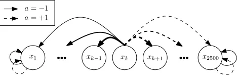
Linear MDP: this problem consists of statesxk∈X,k={1,2, . . . ,2500}arranged in a one-dimensional
chain (see Figure 1). There are two possible actions A={−1,+1} (left/right) and ev-ery state is accessible from any other state except for the two ends of the chain, which are absorbing states. A state xk ∈X is called absorbing if P(xk|xk,a) =1 for all a∈A and P(xl|xk,a) =0,∀l6=k. The state space is of size|X|=2500 and the joint action state space is of size|Z|=5000. Note that naive storing of the model requiresO(107)memory.
The transition probability from an interior statexk to any other state xl is inversely propor-tional to the distance in the direction of the selected action. Formally, consider the following quantityn(xl,a,xk)assigned to all non-absorbing statesxkand to every(xl,a)∈Z:
x1 xk xk xk+1 x2500
−1
a=−1
a= +1
Figure 1: Linear MDP: Illustration of the linear MDP problem. Nodes indicate states. Statesx1and
x2500are the two absorbing states and statexkis an example of interior state. Arrows indi-cate possible transitions ofthese three nodes only. Fromxkany other node is reachable with transition probability (arrow thickness) proportional to the inverse of the distance to
xk(see the text for details).
n(xl,a,xk) =
1
|l−k| for(l−k)a>0
0 otherwise
.
We can write the transition probabilities as
P(xl|xk,a) =
n(xl,a,xk)
∑
xm∈X
n(xm,a,xk) .
Transitions to an absorbing state have associated reward 1 and transitions to any interior state has associated reward−1.
The optimal policy corresponding to this problem is to reach the closest absorbing state as soon as possible.
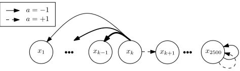
Combination lock: the combination lock problem considered here is a stochastic variant of the reset state space models introduced in Koenig and Simmons (1993), where more than one reset state is possible (see Figure 2).
In our case we consider, as before, a set of statesxk∈X,k∈ {1,2, . . . ,2500}arranged in a one-dimensional chain and two possible actionsA={−1,+1}. In this problem, however, there is only one absorbing state (corresponding to the statelock-opened) with associated reward of 1. This state is reached if the all-ones sequence {+1,+1, . . . ,+1} is entered correctly. Otherwise, if at some statexk,k<2500, action−1 is taken, the lock automatically resets to
some previous statexl,l<krandomly (in the original problem, the reset state is always the
initial statex1).
For every intermediate state, the rewards of actions−1 and+1 are set to 0 and−0.01, re-spectively. The transition probability upon taking the wrong action−1 from statexk to state
x1 xk xk xk+1 x2500 −1
a=−1 a= +1
Figure 2: Combination lock: illustration of the combination lock MDP problem. Nodes indicate states. Statex2500is the goal (absorbing) state and statexkis an example of interior state. Arrows indicate possible transitions ofthese two nodes only. Fromxkany previous state is reachable with transition probability (arrow thickness) proportional to the inverse of the distance toxk. Among the future states onlyxk+1is reachable (arrow dashed).
n(xk,xl) =
1
k−l forl<k
0 otherwise
, P(xl|xk,−1) =
n(xk,xl)
∑
xm∈X
n(xk,xm) .
Note that this problem is more difficult than the linear MDP since the goal state is only reachable from one state,x2499.
Grid world: this MDP consists of a grid of 50×50 states. A set of four actions {RIGHT, UP, DOWN, LEFT}is assigned to every statex∈X. Although the state space of the grid world is of the same size as the previous two problems,|X|=2500, the joint action state space is larger,|Z|=104.
The location of each statexof the grid is determined by the coordinatescx= (hx,vx), wherehx
andvxare some integers between 1 and 50. There are 196 absorbingwall statessurrounding
the grid and another one at the center of grid, for which a reward−1 is assigned. The reward for the walls is
r(x,a) =− 1
kcxk2, ∀a∈A.
Also, we assign reward 0 to all of the remaining (non-absorbing) states.
This means that both the top-left absorbing state and the central state have the least possible reward (−1), and that the remaining absorbing states have reward which increases propor-tionally to the distance to the state in the bottom-right corner (but are always negative).
The transition probabilities are defined in the following way: taking actionafrom any non-absorbing statexresults in a one-step transition in the direction of actionawith probability 0.6, and a random move to a statey6=xwith probability inversely proportional to their Eu-clidean distance 1/kcx−cyk2.
The resulting optimal policy is tosurvivein the grid as long as possible by avoiding both the absorbing walls and the center of the grid. Note that because of the difference between the cost of walls, the optimal control prefers the states near the bottom-right corner of the grid, thus avoiding absorbing states with higher cost.
5.1.1 EXPERIMENTALSETUP ANDRESULTS
For consistency with the theoretical results, we evaluate the performance of all algorithms in terms ofℓ∞-norm error of the action-value functionkQ∗−Qπkkobtained by policyπkinduced at iteration k. The discount factorγis fixed to 0.995 and the optimal action-value functionQ∗is computed with high accuracy through value iteration.
We compare DPP-RL with two other algorithms:
Q-learning (QL): we consider a synchronous variant of Q-learning for which convergence results have been derived in Even-Dar and Mansour (2003). Since QL is sensitive to the learning step, we consider QL with polynomial learning stepαk=1/(k+1)ωwhereω∈ {0.51,0.75,1.0}.
It is known thatωneeds to be larger than 0.5, otherwise QL may not asymptotically converge (see Even-Dar and Mansour, 2003, for the proof).
Model-based Q-value iteration (VI): The VI algorithm (Kearns and Singh, 1999) first estimates a model using all the data samples and then performs value iteration on the learned model. Therefore, unlike QL and DPP, VI is a model-based algorithm and requires the algorithm to store the model.
Comparison between VI and both DPP-RL and QL is especially problematic: first, the number of computations per iteration is different. Whereas DPP-RL and QL require|Z|computations per iteration, VI requires |Z||X|. Second, VI requires to estimate the model initially (using a given number of samples) and then iterates until convergence. This latter aspect is also different from DPP-RL and QL, which use one sample per iteration. Therefore, the number of samples determines the number of iterations for DPP-RL and QL, but not for VI.
For consistency with the theoretical results, we use as error measure, the distance between the optimal action-value function and the value function of the policy induced by the algorithms. instead of the more popular average accumulated reward, which is usually used when the RL algorithm learns from a stream of samples.
Simulations are performed using the following procedure: at the beginning of each run (i)the action-value function and the action preferences are randomly initialized in the interval[−Vmax,Vmax], and(ii)a set of 105samples is generated fromP(·|x,a)for all(x,a)∈Z. As mentioned before, this fixes the maximum number of iterations for DPP-RL and QL to 105, but not for VI. We run VI until convergence. We repeat this procedure 50 times and compute the average error in the end. Using significantly fewer samples leads to a dramatic decrease of the quality of the solutions using all approaches and no qualitative differences in the comparison.
To compare the methods using equivalent logical units independently of the particular imple-mentation, we rescale their number of iterations by the number of steps required in one iteration. For the case of VI, thestepunits are the number of iterations times|Z||X|and for DPP-RL and QL, the number of iterations times|Z|.
0 1 2 3 4 x 10⁸ 10−2
10−1 100 101 102
Linear
Steps
Error
0 1 2 3 4
x 108 10−2
10−1 100 101 102
Combination lock
Steps
0 2 4 6 8
x 108 10−2
10−1 100 101 102
Grid world
Steps
QL (ω=0.51) QL (ω=0.75) QL (ω=1.00) VI DPP−RL
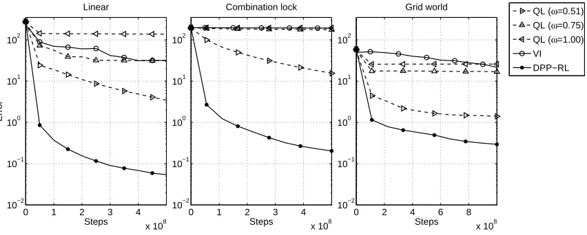
Figure 3: Comparison between DPP-RL, QL and VI in terms ofnumber of steps, defined as the number of iterations times the number of computations per iteration of the particular algorithm. Each plot shows the averaged error of the induced policies over 50 different runs (see the text for details).
at a smaller rate afterwards. We also observe that DPP-RL performs significantly better than QL. The improvement is about two orders of magnitude in both the linear MDP and the combination lock problems and more than four times better in the Grid world. QL shows the best performance forω=0.51 and the quality degrades as a function ofω.
Although the performance of VI looks poor for the number of steps shown in Figure 3, we observe that VI reaches an average error of 0.019 after convergence (≈2·1010steps) for the linear MDP and the combination lock and an error of 0.10 after ≈4·1010 steps for the grid problem. This means for a fixed number of samples, the asymptotic solution of VI is better than the one of DPP-RL, at the cost of much larger number of steps.
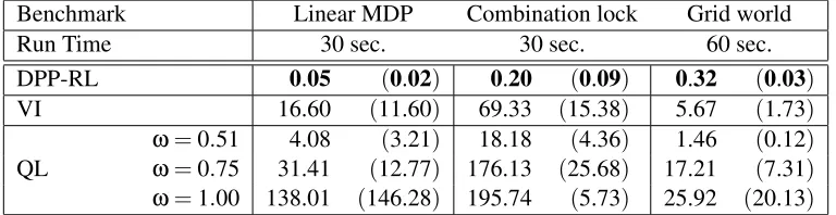
To illustrate the performance of the methods using a limited CPU time budget, we also compare the average and standard deviations of the errors in terms of elapsed CPU time by running the algorithms until a maximum allowed time is reached. We choose 30 seconds in the case of linear MDP and combination lock and 60 seconds for the grid world, which has twice as many actions as the other benchmarks. To minimize the implementation dependent variability, we coded all three algorithms in C++ and ran them on the same processor. CPU time was acquired using the system functiontimes() which provides process-specific CPU time. Sampling time was identical for all methods and not included in the analysis.
Table 1 shows the final average errors (standard deviations between parenthesis) in the CPU time comparison. As before, we observe that DPP-RL converges very fast, achieving near optimal performance after a few seconds. The small variance of estimation of DPP-RL suggests that, as derived in Theorems 9 and 5, DPP-RL manages to average out the simulation noise caused by sampling and converges to a near optimal solution, which is very robust.
Benchmark Linear MDP Combination lock Grid world
Run Time 30 sec. 30 sec. 60 sec.
DPP-RL 0.05 (0.02) 0.20 (0.09) 0.32 (0.03) VI 16.60 (11.60) 69.33 (15.38) 5.67 (1.73)
QL
ω=0.51 4.08 (3.21) 18.18 (4.36) 1.46 (0.12) ω=0.75 31.41 (12.77) 176.13 (25.68) 17.21 (7.31) ω=1.00 138.01 (146.28) 195.74 (5.73) 25.92 (20.13)
Table 1: Comparison between DPP-RL, QL and VI given a fixed computational and sampling bud-get. Table 1 shows error means and standard deviations (between parenthesis) at the end of the simulations for three different algorithms (columns) and three different benchmarks (rows).
for a fixed number of samples, VI obtains a better solution than DPP-RL requiring significantly more computation.
5.2 SADPP
In this subsection, we illustrate the performance of the SADPP algorithm in the presence of func-tion approximafunc-tion and limited sampling budget per iterafunc-tion. The purpose of this subsecfunc-tion is to analyze numerically the sample complexity, that is, the number of samples required to achieve a near optimal performance with low variance.
We compare SADPP withℓ2-regularized versions of the following two algorithms:
Regularized fitted Q-iteration (RFQI) (Farahmand et al., 2008):
RFQI performs value iteration to approximate the optimal action value function. See also Antos et al. (2008) and Ernst et al. (2005).
Regularized Least Squares Policy Iteration (REG-LSPI) (Farahmand et al., 2009):
It can be regarded as a Monte-Carlo sampling implementation of approximate policy iteration (API) with action-state representation (see also Lagoudakis and Parr, 2003).
The benchmark we consider is a variant of theoptimal replacement problempresented in Munos and Szepesv´ari (2008).
5.2.1 OPTIMALREPLACEMENT PROBLEM
This problem is an infinite-horizon, discounted MDP. The state measures the accumulated use of a certain product and is represented as a continuous, one-dimensional variable. At each time-step
t, either the product is kepta(t) =0 or replaceda(t) =1. Whenever the product is replaced by a new one, the state variable is reset to zerox(t) =0, at an additional costC. The new state is chosen according to an exponential distribution, with possible values starting from zero or from the current state value, depending on the latest action:
p(y|x,a=0) = (
βeβ(y−x) ify≥x
0 ify<0 p(y|x,a=1) = (
The reward function is a monotonically decreasing function of the statexif the product is kept
r(x,0) =−c(x)and constant if the product is replacedr(x,1) =−C−c(0), wherec(x) =4x. The optimal action is to keep as long as the accumulated use is below a threshold or to replace otherwise:
a∗(x) = (
0 ifx∈[0,x¯]
1 ifx>x¯ . (11)
Following Munos and Szepesv´ari (2008), ¯xcan be obtained exactly via the Bellman equation and is the unique solution to
C=
Z x¯ 0
c′(y) 1−γ
1−γe−β(1−γ)y
dy.
5.2.2 EXPERIMENTALSETUP ANDRESULTS
For all algorithms we map the state-action space using twenty radial basis functions (ten for the continuous one-dimensional state variable x, spanning the state space X, and two for the two
possible actions). Other parameter values where chosen to be the same as in Munos and Szepesv´ari (2008), that is,γ=0.6,β=0.5,C=30, which results in ¯x≃4.8665. We also fix an upper bound for the states,xmax=10 and modify the problem definition such that if the next statey happens to be outside of the domain[0,xmax]then the product is replaced immediately, and a new state is drawn as if actiona=1 were chosen in the previous time step.
We measure the performance loss of the algorithms in terms of the difference between the optimal action a∗ and the action selected by the algorithms. We use this performance measure since it is easy to compute as we know the analytical solution of the optimal control in the optimal replacement problem (see Equation 11). We discretize the state space inK=100 and compute the error as follows:
Error= 1
K K
∑
k=1
|a∗(xk)−aˆ(xk)|, (12)
where ˆa is the action selected by the algorithm. Note that, unlike RFQI and REG-LSPI, SADPP induces a stochastic policy, that is, a distribution over actions. We select ˆafor SADPP by choosing the most probable action from the induced soft-max policy, and then use this to compute Equation 12. RFQI and REG-LSPI select the action with highest action-value function.
Simulations are performed using the same following procedure for all three algorithms: at the beginning of each run, the vectoreθ0is initialized in the interval[−1,1]. We then let the algorithm run for 103iterations for 200 different runs. A new independent set of samples is generated at each iteration.
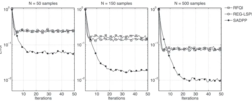
10 20 30 40 50 10−2
10−1 100
N = 500 samples
Iterations
10 20 30 40 50
10−2 10−1 100
N = 50 samples
Erro
r
Iterations
10 20 30 40 50
10−2 10−1 100
N = 150 samples
Iterations
RFQI REG-LSPI SADPP
Figure 4: Numerical results for the optimal replacement problem. Each plot shows the error of RFQI, REG-LSPI and SADPP for certain number of samplesN. Error is defined as in Equation 12 and averaged over 200 repetitions (see the text for details).
Num. samples 50 150 500
SADPP 0.07 (0.06) 0.02 (0.01) 0.01 (0.01) RFQI 0.24 (0.19) 0.17 (0.12) 0.08 (0.07) REG-LSPI 0.26 (0.16) 0.13 (0.10) 0.07 (0.06)
Table 2: Comparison between SADPP, RFQI and REG-LSPI for the optimal replacement problem. Table shows error means and standard deviations (between parenthesis) at the end of the simulations (after 103 iterations) for the three different algorithms (columns) and three different number of samples (rows).
We are interested in the behavior of the error as a function of the iteration number for different number of samplesN per iteration. Figure 4 and Table 2 show the performance results of the three different algorithms for N ∈ {50,150,500} for the first 50 iterations and the total 103 iterations respectively. We observe that after an initial transient, all algorithms reach a nearly optimal solution after 50 iterations.
First, we note that SADPP asymptotically outperforms RFQI and REG-LSPI on average in all cases. Interestingly, there is no significant difference between the performance of RFQI and REG-LSPI. The performance of all algorithms improve for largerN. We emphasize that SADPP using only 50 samples shows comparable results to both RFQI and REG-LSPI using ten times more samples.
Globally, we can conclude that SADPP has positive effects in reducing the effect of simulation noise, as postulated in Section 4. We can also conclude that, for our choice of settings, SADPP outperforms RFQI and REG-LSPI.
6. Related Work
In this section, we review some previous RL methods and compare them with DPP.
Policy-gradient actor-critic methods: As we explained earlier in Section 1, actor-critic method is a popular incremental RL algorithm (Sutton and Barto, 1998; Barto et al., 1983, Chapter 6.6), which makes use of a separate structure to store the value function (critic) and the control pol-icy (actor). An important extension of AC, thepolicy-gradient actor critic(PGAC), extends the idea of AC to problems of practical scale (Sutton et al., 2000; Peters and Schaal, 2008). In PGAC, the actor updates the parameterized policy in the direction of the (natural) gradient of performance, provided by the critic. The gradient update ensures that PGAC asymptotically converges to a local maximum, given that an unbiased estimate of the gradient is provided by the critic (Maei et al., 2010; Bhatnagar et al., 2009; Konda and Tsitsiklis, 2003; Kakade, 2002). The parameterηin DPP is reminiscent of the learning stepβin PGAC methods, since it influences the rate of change of the policy and in this sense may play a similar role as the learning stepβin PGAC (Konda and Tsitsiklis, 2003; Peters and Schaal, 2008). However, it is known that in the presence of sampling error, asymptotic convergence to a local maximum is only attained whenβasymptotically decays to zero (Konda and Tsitsiklis, 2003; Baxter and Bartlett, 2001), whereas the parameterηin DPP, and DPP-RL, can be an arbitrary constant.
Q-learning: DPP is not the only method which relies on an incremental update rule to control the sampling error. There are other incremental RL methods which aim to address the same problem (see, e.g., Maei et al., 2010; Singh et al., 2000; Watkins and Dayan, 1992).
One of the most well-known algorithms of this kind is Q-learning (QL) (Watkins and Dayan, 1992), which controls the sampling error by introducing a decaying learning step to the update rule of value iteration. QL has been shown to converge to the optimal value function in tabular case (Bertsekas and Tsitsiklis, 1996; Jaakkola et al., 1994). Also, there are some studies in the literature concerning the asymptotic convergence of Q-learning in the presence of function approximation (Melo et al., 2008; Szepesv´ari and Smart, 2004). However, the convergence rate of QL is very sensitive to the choice of learning step, and a bad choice of the learning step may lead to a slow rate of convergence (Even-Dar and Mansour, 2003). For instance, the convergence rate of QL with a linearly decaying learning step is of order(1/k)1−γ, which makes the Q-learning algorithm extremely slow for γ≈1 (Szepesv´ari, 1998). This is in contrast to our previously mentioned result on the convergence of DPP-RL in Theorem 10 which guarantees that, regardless of the value ofηandγ, DPP-RL always converges to the optimal policy with a rate of order 1/√k. The numerical results of Section 5.1 confirm the superiority of DPP-RL to QL in terms of the rate of convergence.
One can also compare the finite-time behavior of DPP-RL and QL in terms of the PAC sample complexity of these methods. We have proven a sample-complexity PAC bound of order
Azar et al., 2012, Section 3.3.1).4 This theoretical result suggests that DPP-RL is superior to QL in terms of sample complexity of the estimating the optimal policy, especially, whenγis close to 1.
There is an on-policy version of Q-learning algorithm called SARSA (see, e.g., Singh et al., 2000) which also guarantees the asymptotic convergence to the optimal value function. How-ever little is known about the rate of convergence and the finite-time behavior of this algo-rithm.
Very recently, Azar et al. (2012) propose a new variant of Q-learning algorithm, called speedy Q-learning (SQL), which makes use of a different update rule than standard Q-learning of Watkins and Dayan (1992). Like DPP-RL, SQL converges to the optimal policy with the rate of convergence of order 1/√k. However, DPP-RL is superior to SQL in terms of memory space requirement, since SQL needs twice as much space as DPP-RL does.
Relative-entropy methods: The DPP algorithm is originally motivated (see Appendix A) by the work of Kappen (2005) and Todorov (2007), who formulate a stochastic optimal control problem to find a conditional probability distribution p(y|x) given an uncontrolled dynam-ics ¯p(y|x). The control cost is the relative entropy between p(y|x)and ¯p(y|x)exp(r(x)). The difference is that in their work a restricted class of control problems is considered for which the optimal solutionpcan be computed directly in terms of ¯pwithout requiring Bellman-like iterations. Instead, the present approach is more general, but does require Bellman-like iter-ations. Likewise, our formalism is superficially similar to PoWER (Kober and Peters, 2009) and SAEM (Vlassis and Toussaint, 2009), which rely on EM algorithm to maximize a lower bound for the expected return in an iterative fashion. This lower-bound also can be writ-ten as a KL-divergence between two distributions. Also, the natural policy gradient method can be seen as a relative entropy method, in which the second-order Taylor expansion of the relative-entropy between the distribution of the states is considered as the metric for policy improvement (Bagnell and Schneider, 2003). Another relevant study isrelative entropy policy search(REPS) (Daniel et al., 2012; Peters et al., 2010) which relies on the idea of minimizing the relative entropy to control the size of policy update. However there are some differences between REPS and DPP.(i)In REPS the inverse temperatureηneeds to be optimized while DPP converges to the optimal solution for any inverse temperatureη, and(ii)unlike DPP, no convergence analysis is presented REPS.
7. Discussion and Future Work
We have presented a new approach, dynamic policy programming (DPP), to compute the optimal policy in infinite-horizon discounted-reward MDPs. We have theoretically proven the convergence of DPP to the optimal policy for the tabular case. We have also provided performance-loss bounds for DPP in the presence of approximation. The bounds have been expressed in terms of supremum
4. Note that Even-Dar and Mansour (2003) make use of a slightly different performance measure than the one we use in this paper: The optimized result of Even-Dar and Mansour (2003), which is of order O(1/(1−γ)5), is a bound on the sample complexity of estimatingQ∗withεprecision, whereas in this paper we consider the sample complexity of finding anε-optimal policy. However, the latter can be easily derived for QL from the inequality
kQ∗−Qπkk ≤1/(1−γ)kQ∗−Q
kk, whereπkis the greedy policy w.r.t. QkandQkis the estimate of action-value
norm of average accumulated error as opposed to the standard bounds which are expressed in terms of supremum norm of the errors. We have then introduced a new incremental RL algorithm, called DPP-RL, which relies on a sample estimate instance of the DPP update rule to estimate the optimal policy. We have proven that DPP-RL converges to the optimal policy with the rate of 1/√k.
We have also compared numerically the finite-time behavior of DPP-RL with similar RL meth-ods. Experimental results have shown a better performance of DPP-RL when compared to QL and VI in terms of convergence rate. In these problems, for equal number of samples, VI converged to a better solution than DPP-RL, at the cost of many more steps. When compared to VI, DPP-RL does not need to store the model dynamics, resulting in significantly less memory requirements for large-scale MDPs. This statement is general and holds when comparing DPP-RL to any model-based method.
We have proposed SADPP as a variant of DPP which makes use of linear function approxi-mation and regularization. SADPP has been shown to perform better than two other regularized methods, RFQI and REG-LSPI. We think that this is mainly due to the reduction of the effect of simulation noise (Section 4). At the same time, we admit that the existence of an additional param-eterηfavors SADPP since SADPP performs best for a finite-value ofη. Therefore, it is interesting to consider soft-max variants of RFQI and LSPI which also make use of the inverse temperatureη. In these cases,ηshould be initialized at a finite value and would gradually grow to+∞.
The empirical comparison with those methods that do not make use of generative model as-sumption is outside of the scope of the current work and is left for future research. These methods include, for instance, PGAC methods that use sequences of samples to learn the value function of the current policy (Peters and Schaal, 2008; Konda and Tsitsiklis, 2003; Sutton et al., 2000), or upper-confidence bounds methods which address the exploration-exploitation dilemma (Jaksch et al., 2010; Szita and Szepesv´ari, 2010; Bartlett and Tewari, 2009; Strehl et al., 2009).
Another interesting line of future research is to devise finite-sample PAC bounds for SADPP in the spirit of previous theoretical results available for fitted value iteration and fittedQ-iteration (Munos and Szepesv´ari, 2008; Antos et al., 2008; Munos, 2005). This would require extending the error propagation result of Theorem 5 to an ℓ2-norm analysis and combining it with the standard regression bounds.
Finally, an important extension of our results would be to apply DPP to large-scale action prob-lems. This would require an efficient way to approximateMηΨk(x)in the update rule of Equation 5,
since computing the exact summations becomes expensive. One idea is to sample estimateMηΨk(x)
using Monte-Carlo simulation (MacKay, 2003, Chapter 29), sinceMηΨk(x)is the expected value
ofΨk(x,a)under the soft-max policyπk.
Acknowledgments
Appendix A. From Bellman Equation to DPP Recursion
In this appendix, we give an informalderivationof the DPP equation. This is only for helping the reader to understand the origin of the DPP equation and it is in no way meant as a justification of DPP. The theoretical analysis and the proof of convergence of DPP is provided in Section 3.2.
Let ¯πbe a stochastic policy, that is, ¯π(a|x)>0 for all(x,a)∈Z. Consider the relative entropy between the policyπand some baseline policy ¯π:
gππ¯(x),KL(π(·|x)kπ¯(·|x)) =
∑
a∈A
π(a|x)log
π(a|x) ¯ π(a|x)
, ∀x∈X.
Note that gππ¯(x) is a positive function of x which is also bounded from above due to the as-sumption that ¯πis a stochastic policy. We define a new value function Vπ¯π, for all x∈X, which incorporates g as a penalty term for deviating from the base policy ¯π and the reward under the policyπ:
Vπ¯π(x), nlim →∞E
"
n
∑
k=0 γk
rt+k−
1 ηg
π ¯ π(xt+k)
xt =x
#
,
whereηis a positive constant andrt+kis the reward at timet+k. Also, the expected value is taken
w.r.t. the state transition probability distribution Pand the policy π. The optimal value function
Vπ¯∗(x),supπVπ¯π(x) then exists and is bounded by some finite constant c >0. Also, the value functionVπ¯∗(x)satisfies the following Bellman equation for allx∈X:
Vπ¯∗(x) = sup π(·|x)a
∑
∈Aπ(a|x)
r(x,a)−1 ηlog
π(a|x) ¯
π(a|x)+γ(PV ∗ ¯ π)(x,a)
. (13)
Equation 13 is a modified version of Equation 2 where, in addition to maximizing the expected reward, the optimal policy ¯π∗ also minimizes the distance with the baseline policy ¯π. The max-imization in Equation 13 can be performed in closed form. Following Todorov (2007), we state Proposition 1 (closely related results to Proposition 1 can be found in the recent works of Still and Precup, 2012; Peters et al., 2010):
Proposition 1 Letηbe a positive constant, then for all x∈Xthe optimal value function Vπ¯∗(x)and for all(x,a)∈Zthe optimal policyπ¯∗(a|x), respectively, satisfy:
Vπ¯∗(x) = 1
ηloga
∑
∈Aπ¯(a|x)expη(r(x,a) +γ(PVπ¯∗)(x,a))
,
¯
π∗(a|x) =π¯(a|x)exp
η(r(x,a) +γ(PVπ¯∗)(x,a))
exp(ηVπ¯∗(x)) . (14) Proof We must optimizeπsubject to the constraints∑a∈Aπ(a|x) =1 and 0<π(a|x)<1. We define
the Lagrangian functionL(x;λx):X→ℜby adding the termλx
∑a∈Aπ(a|x)−1
L(x;λx) =
∑
a∈Aπ(a|x) [r(x,a) +γ(PVπ¯∗) (x,a)]−1
ηKL(π(·|x)kπ¯(·|x))−λx "
∑
a∈A
π(a|x)−1 #
.
The maximization in Equation 13 can be expressed as maximizing the Lagrangian function L(x,λx). The necessary condition for the extremum with respect toπ(·|x)is:
0=∂L(x,λx)
∂π(a|x) =r(x,a) +γ(PVπ¯∗) (x,a)− 1 η−
1 ηlog
π(a|x)
¯ π(a|x)
−λx,
which leads to
¯
π∗(a|x) =π¯(a|x)exp(−ηλx−1)exp[η(r(x,a) +γ(PVπ¯∗) (x,a))], ∀x∈X. (15) The Lagrange multipliers can then be solved from the constraints:
1=
∑
a∈A
¯
π∗(a|x) =exp(−ηλx−1)
∑
a∈A¯
π(a|x)exp[η(r(x,a) +γ(PVπ¯∗) (x,a))],
λx=
1 ηloga
∑
∈A
¯
π(a|x)exp[η(r(x,a) +γ(PVπ¯∗) (x,a))]−1
η. (16)
By plugging Equation 16 into Equation 15 we deduce
¯
π∗(a|x) = π¯(a|x)exp[η(r(x,a) +γ(PVπ¯∗) (x,a))] ∑
a∈A
¯
π(a|x)exp[η(r(x,a) +γ(PVπ¯∗) (x,a))], ∀(x,a)∈Z. (17) The results then follows by substituting Equation 17 in Equation 13.
The optimal policy ¯π∗is a function of the base policy, the optimal value functionVπ¯∗and the state transition probabilityP. One can first obtain the optimal value functionVπ¯∗ through the following fixed-point iteration:
Vπ¯k+1(x) = 1
ηloga
∑
∈Aπ¯(a|x)expη(r(x,a) +γ(PVπ¯k)(x,a)), (18) and then compute ¯π∗using Equation 14. ¯π∗maximizes the value functionVπ¯π. However, we are not, in principle, interested in quantifying ¯π∗, but in solving the original MDP problem and computing π∗. The idea to further improve the policy towardsπ∗is to replace the base-line policy with the just newly computed policy of Equation 14. The new policy can be regarded as anew base-line policy, and the process can be repeated again. This leads to a double-loop algorithm to find the optimal policyπ∗, where the outer-loop and the inner-loop would consist of a policy update, Equation 14, and a value function update, Equation 18, respectively.
Vπ¯k+1(x) = 1
ηloga
∑
∈Aπ¯k(a|x)expη(r(x,a) +γ(PVπ¯k)(x,a)), (19)
¯
πk+1(a|x) = ¯
πk(a|x)exp
η(r(x,a) +γ(PVπ¯k)(x,a))
exp ηVπ¯k+1(x) . (20) Further,(ii)we define the action preference function Ψk(Sutton and Barto, 1998, Chapter 6.6),
for all(x,a)∈Zandk≥0, as follows:
Ψk+1(x,a), 1
ηlog ¯πk(a|x) +r(x,a) +γ(PV
k
¯
π)(x,a). (21)
By comparing Equation 21 with Equation 20 and Equation 19, we deduce
¯
πk(a|x) =
exp(ηΨk(x,a))
∑
a′∈A
exp(ηΨk(x,a′))
, (22)
Vπ¯k(x) = 1 ηloga
∑
∈A
exp(ηΨk(x,a))). (23)
Finally,(iii)by plugging Equation 22 and Equation 23 into Equation 21 we derive
Ψk+1(x,a) =Ψk(x,a)−LηΨk(x) +r(x,a) +γ(PLηΨk)(x,a), (24)
withLηoperator being defined byLηΨ(x),1ηlog∑a∈Aexp(ηΨ(x,a)). Equation 24 is one form
of the DPP equations. There is an analytically more tractable version of the DPP equation, where we replace Lη by the Boltzmann soft-max Mη defined by MηΨ(x) ,
∑a∈A
exp(ηΨ(x,a))Ψ(x,a)∑a′∈Aexp(ηΨ(x,a′))
.5 In principle, we can provide formal analy-sis for both versions. However, the proof is somewhat simpler for theMηcase, which we make use of it in the rest of this paper. By replacingLη withMηwe deduce the DPP recursion:
Ψk+1(x,a) =OΨk(x,a),Ψk(x,a) +r(x,a) +γPMηΨk(x,a)−MηΨk(x)
=Ψk(x,a) +TπkΨk(x,a)−πkΨk(x)
, ∀(x,a)∈Z,
whereOis an operator defined on the action preferencesΨkandπkis the soft-max policy associated
withΨk:
πk(a|x),
exp(ηΨk(x,a))
∑
a′∈A
exp(ηΨk(x,a′)) .
5. ReplacingLηwithMηis motivated by the following relation between these two operators:
|LηΨ(x)−MηΨ(x)|=1/ηHπ(x)≤log(| A|)
η , ∀x∈X, (25)
withHπ(x)is the entropy of the policy distributionπobtained by pluggingΨinto Equation A. In words,MηΨ(x)is
Appendix B. The Proof of Convergence of DPP—Theorem 2 and Theorem 4
In this section, we provide a formal analysis of the convergence behavior of DPP.
B.1 Proof of Theorem 2
In this subsection we establish a rate of convergence for the value function of the policy induced by DPP. The main result is in the form of following finite-iteration performance-loss bound, for all
k≥0:
kQ∗−Qπkk ≤
2γ4Vmax+log(|
A|)
η
(1−γ)2(k+1) . (26) Here,Qπkis the action-values under the policyπ
kandπk is the policy induced by DPP at stepk.
To derive Equation 26 one needs to relateQπk to the optimalQ∗. Unfortunately, finding a direct
relation betweenQπkandQ∗is not an easy task. Instead, we relateQπktoQ∗via an auxiliary
action-value functionQk, which we define below. In the remainder of this Section we take the following
steps:(i)we expressΨkin terms ofQk in Lemma 13.(ii)we obtain an upper bound on the normed
error kQ∗−Qkk in Lemma 14. Finally, (iii) we use these two results to derive a bound on the normed errorkQ∗−Qπkk. For the sake of readability, we skip the formal proofs of the lemmas in
this section since we prove a more general case in Section C.
Now let us define the auxiliary action-value functionQk. The sequence of auxiliary action-value
functions{Q0,Q1,Q2, . . .}is obtained by iterating the initialQ0=Ψ0from the following recursion:
Qk=k−1
k T
πk−1Q k−1+
1
kT
πk−1Q
0, (27)
whereπkis the policy induced by thekthiterate of DPP.
Lemma 13 relatesΨkwithQk:6
Lemma 13 Let k be a positive integer. Then, we have
Ψk=kQk+Q0−πk−1((k−1)Qk−1+Q0). (28) The following lemma relatesQkandQ∗:
Lemma 14 Let Assumption 1 hold and k be a positive integer. Also assume thatkΨ0k ≤Vmax. Then
the following inequality holds:
kQ∗−Qkk ≤
γ4Vmax+log(|
A|)
η
(1−γ)k .
Lemma 14 provides an upper bound on the normed-errorQk−Q∗. We make use of Lemma 14 to prove the main result of this Subsection: