Published online January 07, 2015 (http://www.sciencepublishinggroup.com/j/acm) doi: 10.11648/j.acm.20140306.19
ISSN: 2328-5605 (Print); ISSN: 2328-5613 (Online)
A cubic Bézier model with shape parameters
Juncheng Li
Department of Mathematics, Hunan University of Humanities, Science and Technology, Loudi, China
Email address:
lijuncheng82@126.com
To cite this article:
Juncheng Li. A Cubic Bézier Model with Shape Parameters. Applied and Computational Mathematics. Vol. 3, No. 6, 2014, pp. 343-348. doi: 10.11648/j.acm.20140306.19
Abstract:
A novel extension of the cubic Bézier curve with two shape parameters is presented in this work. The proposed curve is still a cubic polynomial model, which has simpler structure than other similar models. The proposed curve has the same properties with the usual cubic Bézier curve and its shape can be adjusted by altering values of the two shape parameters while the control points are fixed. With the two shape parameters, the proposed curve can approach to its control polygon farther or closer. The corresponding surface with four shape parameters has the similar properties with the proposed curve and enjoys the shape adjustable property.Keywords:
Cubic Bézier Curve, Cubic Polynomial, Shape Parameter, Shape Adjustment1. Introduction
In Computer Aided Geometric Design (CAGD), the cubic Bézier curve and surface have been widely used for geometric modeling. However, when the control points are given, the shapes of the usual cubic Bézier curve and surface cannot be changed. With the development of geometric design industry, shapes of curves and surface often need to be changed freely. Hence, shapes of the usual cubic Bézier curve and surface cannot be modified limit their practical applications in geometric modeling. For relieving the default of the usual cubic Bézier curve and surface, the Bézier-like curves and surfaces with shape parameters have been paid more and more attention by many researchers.
At present, in order to introduce shape parameters to the usual cubic Bézier curve and surface, the most commonly used methods have two kinds. One is to construct the quasi cubic Bézier curves and surfaces with shape parameters based on the space with trigonometric or hyperbolic functions, such as [1-8], another is to construct the high-degree Bézier curves and surfaces with shape parameters by increasing the degree of the Bernstein basis, such as [9-14]. Although those methods can effectively realize the shape adjustment of the curves and surfaces by altering the values of the shape parameters, the structure complexity is thereupon increased. The Bézier curve and surface with multiple shape parameters of the same degree [15] was a novel method, but the curve and surface did not have the strict symmetry that the usual Bézier curve and surface have. The main purpose of this work is to present
another novel extension of the cubic Bézier curve and surface with shape parameters. The shape of the proposed curve and surface can be adjusted by altering values of the shape parameters when the control points are fixed. More important, the proposed curve and surface are still cubic polynomial models and has the same properties with the usual cubic Bézier models.
The rest of this paper is organized as follows. In Section 2, the cubic Bézier basis with two shape parameters (αβ-Bézier basis for short) is constructed, and some properties of the basis are given. In Section 3, the corresponding curve with two shape parameters (αβ-Bézier curve for short) is defined, the properties of the αβ-Bézier curve are discussed and effects of the shape parameters on αβ-Bézier curve are studied. In Section 4, the corresponding surface with four shape parameters (αβ-Bézier surface for short) is presented. A short conclusion is given in Section 5.
2. αβ-Bézier Basis
The construction process of a class of cubic Bézier basis with two shape parameters α and β (αβ-Bézier basis for short) are given as below.
[
]
2 3 0( )
1( )
2( )
3( )
1
f t
f t
f t
f t
=
t t
t M
(1)where t∈[0, ]α (0< ≤α 1) , and M is an undetermined
4 4× matrix.
Derivation calculus to Eq. (1), then
[
]
20( ) 1( ) 2( ) 3( ) 0 1 2 3
f t′ f t′ f t′ f t′ = t t M (2)
The αβ-Bézier basis is hoped to satisfy the similar properties with the usual cubic Bernstein basis functions at the end point. Let t=0 and t=α in Eq. (1) and Eq. (2) respectively, then
[
1 0 0 0] [
= 1 0 0 0]
M (3)[
]
2 30 0 0 1 =1 α α α M (4)
[
−β β 0 0] [
= 0 1 0 0]
M (5)[
]
20 0 −β β =0 1 2α 3α M (6) From Eq. (3) to Eq. (6), then
2 3
2
1 0 0 0 1 0 0 0
0 0 0 1 1
0 0 0 1 0 0
0 0 0 1 2 3
M
α α α β β
β β α α
= − − (7)
Solving Eq. (7) and taking the result to Eq. (1), the
αβ-Bézier basis can be defined as follows.
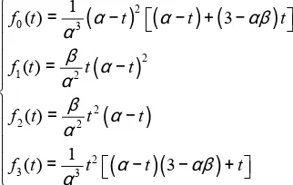
Definition 1. For two arbitrary selected real values of
α(0< ≤α 1) and β(0< ≤β 3), the following four functions
of t(0≤ ≤t α) are called the cubic Bézier basis with two shape parameters α and β (αβ-Bézier basis for short),
(
) (
) (
)
(
)
(
)
(
)(
)
2 0 3 2 1 2 2 2 2 2 3 3 1( ) 3
( )
( )
1
( ) 3
= − − + − = − = − = − − +
f t t t t
f t t t
f t t t
f t t t t
α α αβ
α β α α β α α α αβ α (8)
Theorem 1. The αβ-Bézier basis defined as Eq. (8) has the following properties,
(a) Nonnegativity: f ti( )≥0 (i=0,1, 2, 3).
(b) Degeneration: For α =1 and β =3, the αβ-Bézier basis degenerates into the usual cubic Bernstein basis.
(c) Monotonicity: For fix t∈
[ ]
0,α and α∈(0,1], f t0( )and f t3( ) are monotonically decreasing about β , f t1( )
and f t2( ) are monotonically increasing about β.
(d) Partition of unity:
0( ) 1( ) 2( ) 3( ) 1
f t + f t + f t + f t ≡ .
(e) Symmetry:
3
( ; , ) ( ; , )
i i
f t α β = f − α−tα β (i=0,1, 2, 3).
(f) Properties at the endpoints:
0 1 2 3
0 1 2 3
(0) 1, (0) (0) (0) 0
( ) ( ) ( ) 0, ( ) 1
f f f f
f α f α f α f α
= = = =
= = = =
(9)
0 1
2 3
0 1
2 3
(0) , (0) ,
(0) 0, (0) 0,
( ) 0, ( ) 0,
( ) , ( ) . f f f f f f f f β β α α
α β α β
′ = − ′ = ′ ′ = = ′ = ′ = ′ = − ′ = (10)
Proof. (a) For 0≤ ≤t α , 0< ≤α 1 and 0< ≤β 3, then 0
t
α− ≥ , 3−αβ ≥0. From Eq. (8), f ti( )≥0 (i=0,1, 2, 3) follow obviously.
(b) For α =1 and β =3, the αβ-Bézier basis can be expressed as follows,
( )
( )
( )
3 0 2 1 2 2 3 3( ) 1
( ) 3 1
( ) 3 1
( )
f t t
f t t t f t t t f t t
= − = − = − = (11)
Eq. (11) is the expression of the usual cubic Bernstein basis exactly, which shows that the αβ-Bézier basis degenerates into the cubic Bernstein basis functions when α =1 and β =3.
(c) For t∈
[ ]
0,α and α∈(0,1], then2 0
2
d
( ) 0
d
f t
t α
β = −α − ≤ ,
2 1
2
d
( ) 0
d f t
t α
β α= − ≥ ,
2 2
2
d
( ) 0
d f t
t α
β α= − ≥ ,
2 3
2
d
( ) 0
d
f t
t α
α = −α − ≤ .
Hence, f t0( ) and f t3( ) are monotonically decreasing about β , f t1( ) and f t2( ) are monotonically increasing
about β.
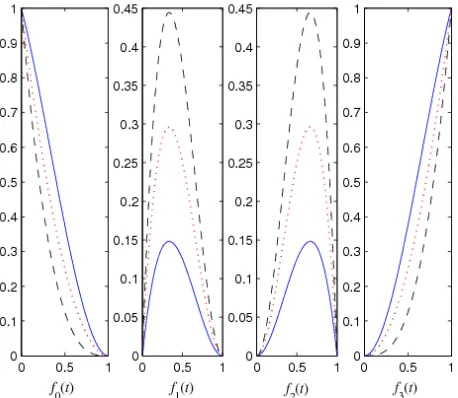
By simple deduction, the remaining cases follow obviously. Fig. 1 and Fig. 2 show curves of the αβ-Bézier basis for different values of α and β. In Fig. 1, the value of β is set forβ =3, and the value of α is set for α =0.4(solid lines), α =0.8 (dotted lines) and α =1.0 (dashed lines) respectively. In Fig. 2, the value of α is set for α =1.0, and
the value of β is set for β =1.0 (solid lines),
2.0
β = (dotted lines) and β =3.0 (dashed lines)
Figure 1. Curves of the αβ-Bézier basis for different values of α
Figure 2. Curves of the αβ-Bézier basis for different values of β
3. αβ-Bézier Curve
3.1. Definition and Properties of the αβ-Bézier Curve
On the base of the αβ-Bézier basis, the corresponding curve with two shape parameters can be defined as follows.
Definition 2. Given pi (i=0,1, 2, 3) are four control points
in R2 or R3, for 0≤ ≤t α, 0< ≤α 1 and 0< ≤β 3, then
3
0
( ) i( ) i i
t f t
=
=
∑
B p (12)
is called the cubic Bézier curve with two shape parameters α
and β (αβ-Bézier curve for short), where f ti( ) (i=0,1, 2, 3)
are the αβ-Bézier basis defined as Eq. (8).
Remark 1. The curve defined as Eq. (12) can be reparametrized to a new curve by R( )u =B(αu). Then R( )u
is defined on a fixed interval [0,1] . For given control points
i
p (i=0,1, 2, 3), both B( )t and B( )u represent the same curve. The curve with B( )t is used in the following discussion.
From the properties of the αβ-Bézier basis and definition of the αβ-Bézier curve, some properties of the αβ-Bézier curve can be obtained as follows.
Theorem 2. The αβ-Bézier curve defined as Eq. (12) has the following properties,
(a) Terminal properties: The curve interpolates the first and the end control points and tangent to the first and the end edges of the control polygon, i.e.,
0
3
1 0
3 2
(0) ( )
(0) ( )
( ) ( )
α β α β
=
=
′ = −
′ = −
B p
B p
B p p
B p p
(b) Symmetry: For the same shape parameter
α (0< ≤α 1) and β (0< ≤β 3) , both pi and
3−i
p (i=0,1, 2, 3) define the same curve in a different parameterization, i.e.,
0 1 2 3 3 2 1 0
( ;t , , , )= (α−t; , , , )
B p p p p B p p p p
where 0≤ ≤t α.
(c) Geometric invariant and affine invariance: Location and shape of the curve depend only on the four control points
i
p (i=0,1, 2, 3), the parameter α and β, regardless of the choice of coordinate system, i.e., shape of the curve will keep unchanged after rotation and coordinate translation. In addition, after implementing affine transformation to the control points, the new curve will correspond to the same affine transformation curve.
(d) Convex hull property: A curve with B( )t must lie inside its control polygons span by pi (i=0,1, 2, 3).
Proof. (a) From Eq. (9) and Eq. (12), then
0 0 1 1 2 2 3 3 0
(0)= f (0) + f(0) + f (0) + f (0) =
B p p p p p
0 0 1 1 2 2 3 3 3
( )α = f ( )α + f( )α + f ( )α + f ( )α =
B p p p p p
From Eq. (10) and Eq. (12), then
0 0 1 1 2 2 3 3
0 1 1 0
(0) (0) (0) (0) (0)
( )
f f f f
β β β
′ = ′ + ′ + ′ + ′
= − + = −
B p p p p
p p p p
0 0 1 1 2 2 3 3
3 2 3 2
( ) ( ) ( ) ( ) ( )
( )
f f f f
α α α α α
β β β
′ = ′ + ′ + ′ + ′
= − + = −
B p p p p
p p p p
(b) For the same shape parameter α (0< ≤α 1) and
3 2 1 0
0 3 1 2 2 1 3 0
3 3 2 2 1 1 0 0
0 1 2 3
( ; , , , )
( ) ( ) ( ) ( )
( ) ( ) ( ) ( )
( ; , , , )
t
f t f t f t f t
f t f t f t f t t
α
α α α α
−
= − + − + − + −
= + + +
=
B p p p p
p p p p
p p p p B p p p p
(c) Because of the parametric form of the curve, this property follows obviously.
(d) This property follows since the αβ-Bézier basis satisfies nonnegative property and sums to one which are shown in Theorem 1.
Remark 2. Theorem 2 shows that the αβ-Bézier curve inherits the same properties with the usual cubic Bézier curve. Particularity, the αβ-Bézier curve degenerates into the usual cubic Bézier curve when α=1 and β =3. Therefore, the
αβ-Bézier curve is an extension of the usual cubic Bézier curve.
Remark 3. There are many cubic Bézier-like curves with shape parameters had been constructed by some researchers. They introduce the shape parameters through modifying the polynomial functions of the usual cubic Bézier curve to trigonometric or hyperbolic functions [1-8], or increasing the degree of the usual cubic Bézier curve [9-14]. The shapes of those curves can be adjusted by altering values of the shape parameters, but the structure complexity is thereupon increased. Although Xiang, et al [15] constructed a cubic Bézier curve with shape parameters of the same degree, the curve did not have the strict symmetry that the usual cubic Bézier curve has. In contrast with those similar curves, the
αβ-Bézier curve presented in this work has the following characteristic,
(a) In contrast with the quasi cubic Bézier curve with the parameter [1-8], the αβ-Bézier curve is a cubic polynomial curve. Hence, structure of the αβ-Bézier curve is simpler than those curves based on the space with trigonometric or hyperbolic functions.
(b) In contrast with the high-degree Bézier curve with the parameter [9-14], the αβ-Bézier curve is still a cubic polynomial model. Hence, formula complexity of the
αβ-Bézier curve is simpler than those curves constructed by increasing the degree of the Bernstein basis functions.
(c) In contract with the Bézier curve with multiple parameters of the same degree [15], the αβ-Bézier curve satisfies strict symmetry that the usual cubic Bézier curve has. Hence, the αβ-Bézier curve is more suitable in practical engineering than the curve didn’t satisfy strict symmetry.
3.2. Effects of the Shape Parameters on αβ-Bézier Curve
When the four control points are fixed, shape of the usual cubic Bézier curve cannot be changed, while shape of the proposed curve can be adjusted by altering values of the shape parameter α(0< ≤α 1) and β (0< ≤β 3). Effects of the shape parameters on the αβ-Bézier curve approaches to its polygon are shown as follows.
Theorem 3. Suppose pi (i=0,1, 2, 3) are not collinear,
and p0, p3 lie on the same side of edge p p0 3, the shape parameters α and β have the following effects on the αβ-Bézier
curve,
(a) When β is fixed, the αβ-Bézier curve approaches closer to its control polygon as α increases.
(b) When α is fixed, the αβ-Bézier curve approaches closer to its control polygon as β increases
(c) The αβ-Bézier curve approaches closer to its control polygon as α and β increase simultaneously.
Proof. Let 1 2
2
* = p +p
p , from Eq. (12), then
(
0 1 2 3)
4
2 8
α −αβ
− = − − +
*
B p p p p p (13)
where 0< ≤α 1, 0< ≤β 3. Taking the norm in Eq. (13), then
0 1 2 3
4
2 8
α −αβ
− = − − +
*
B p p p p p (14)
From Eq. (14), then
(a) When β is fixed, since 4 8
αβ
−
decreases as α increases,
the αβ-Bézier curve approaches closer to its control polygon with the increase of α.
(b) When α is fixed, since 4 8
αβ
−
decreases as β increases,
the αβ-Bézier curve approaches closer to its control polygon with the increase of β.
(c) Since 4 8
αβ
−
decreases as α and β simultaneously
increase, the αβ-Bézier curve approaches closer to its control polygon with the simultaneous increase of α and β.
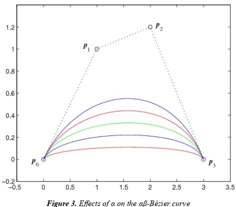
Figure 3. Effects of α on the αβ-Bézier curve
Fig. 3 shows the αβ-Bézier curve corresponding to the same
control polygon by fixing β =2 and setting
0.2, 0.4, 0.6, 0.8,1.0
α = respectively from outside to inside.
Fig. 4 shows the αβ-Bézier curve corresponding to the same
0.5,1.0,1.5, 2.0, 2.5, 3.0
β = respectively from outside to
inside.
Figure 4. Effects of β on the αβ-Bézier curve
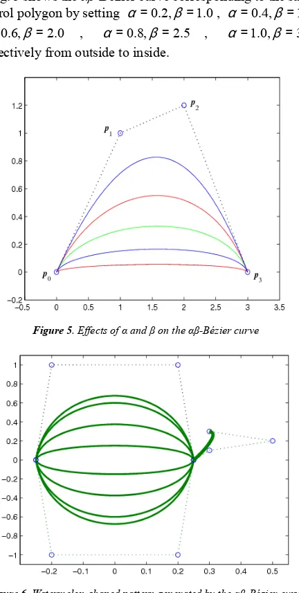
Fig. 5 shows the αβ-Bézier curve corresponding to the same control polygon by setting α=0.2,β=1.0, α =0.4,β =1.5,
0.6, 2.0
α= β = , α =0.8,β =2.5 , α =1.0,β =3.0 respectively from outside to inside.
Figure 5. Effects of α and β on the αβ-Bézier curve
Figure 6. Watermelon-shaped pattern generated by the αβ-Bézier curve
The watermelon-shaped pattern generated by altering values of the shape parameters α and β is shown in Fig. 6.
4. αβ-Bézier Surface
Using tensor product, the corresponding surface with four shape parameters can be defined as follows.
Definition 3. Given pi j, ( ,i j=0,1, 2, 3) are 4×4 control
points in 3
R , f ui( )(0≤ ≤u α1, 0<α1≤1, 0<β1≤3) and
( )
j
f v (0≤ ≤u α2 , 0<α2 ≤1, 0<β2 ≤3) are the basis defined according to Eq. (8), then
3 3
,
0 0
( , ) i( ) j( ) i j
i j
u v f u f v
= =
=
∑∑
B p (15)
is called the cubic Bézier surface with four shape parameters
i
α and βi (i=1, 2) (αβ-Bézier surface for short).
The αβ-Bézier surface defined as Eq. (15) has symmetry, geometric invariant and convex hull property that the usual cubic Bézier surface has. Particularity, the αβ-Bézier surface degenerates into the usual Bézier surface when αi =1 and
3
i
β = (i=1, 2). When the control mesh is fixed, shape of the
αβ-Bézier surface can be adjusted by altering values of the four shape parameters αi and βi (i=1, 2).
Fig. 7 shows the αβ-Bézier surface corresponding to the same control mesh by setting different values of the shape
parameters α αi = and βi =β (i=1, 2) , where (a)
0.5, 1.0
α = β = , (b) α =1.0,β =1.0, (c) α =0.8,β=2.0,
(d) α =0.8,β =3.0.
Figure 7. The αβ-Bézier surface for different values of shape parameters
5. Conclusions
As mentioned above, the αβ-Bézier curve not only has the same properties with the usual cubic Bézier curve, but also can be easily adjusted by altering values of the shape parameters when the control points are fixed. More important, the
simpler structure than other similar models. The αβ-Bézier surface also has the same properties with the usual cubic Bézier surface and its shape can be adjusted by altering values of the shape parameters while the control mesh is kept unchanged. Because there is nearly no difference in structure between the αβ-Bézier models and the usual cubic Bézier models, it is no difficult to adopt the αβ-Bézier models to a CAD/CAM system that already uses the usual cubic Bézier models.
For practical applications of αβ-Bézier models in geometric modeling, it is clear that some special algorithms need to be established. Some interesting results in this area will be discussed in the following study.
Acknowledgments
This work was supported by the Hunan Provincial Natural Science Foundation of China under grant number 13JJ6081 and Scientific Research Fund of Hunan Provincial Education Department of China under grant number 14B099. The author is also very grateful to the Hunan provincial key construction discipline “Computer Application Technology” of Hunan University of Humanities, Science and Technology of China.
References
[1] J. W. Zhang, “C-Bézier curves and surfaces”, Graphical Models and Image Processing, vol. 61, no. 1, pp. 2-15, 1999. [2] Q. Y. Chen and G. Z. Wang, “A class of Bézier-like curves”,
Computer Aided Geometric Design, vol. 20, no. 1, pp. 29–39, 2003.
[3] J. W. Zhang, F. L. Krause and H. Y. Zhang. “Unifying C-curves and H-curves by extending the calculation to complex numbers”, Computer Aided Geometric Design, vol. 22, no. 9, pp. 865-883, 2005.
[4] X.-A. Han, Y. C. Ma and X. L. Huang, “The cubic trigonometric Bézier curve with two shape parameters”,
Applied Mathematical Letters, vol. 22, no. 2, pp. 226-231, 2009.
[5] J. C. Li, D. B. Zhao, B. J. Li and G. H. Chen, “A family of quasi-cubic trigonometric curves”, Journal of Information and Computational Science, vol. 7, no. 13, pp. 2847-2854, 2010. [6] X. L. Han and Y. P. Zhu, “Curve construction based on five
trigonometric blending functions”, BIT Numerical Mathematics, vol. 52, no. 4, pp. 953-979, 2012.
[7] J. C. Li, “A class of cubic trigonometric Bézier curve with a shape parameter”, Journal of Information and Computational Science, vol. 10, no.10, pp. 3071-3078, 2013.
[8] U. Bashir, M. Abbsa and J. M.Ali, “The G2 and C2 rational quadratic trigonometric Bézier curve with two shape parameters with applications”, Applied Mathematics and Computation, vol. 219. no. 20, pp. 10183-10197, 2013. [9] W. T. Wang and G. Z. Wang, “Bézier curves with shape
parameters”, Journal of Zhejiang University SCIENCE A, vol. 6, no. 6, pp. 497-501, 2005.
[10] X.-A. Han, Y. C. Ma and X. L.Huang, “A novel generalization of Bézier curve and surface”, Journal of Computational and Applied Mathematics, vol. 217, no. 1, pp. 180-193, 2008. [11] L. Q. Yang and X M. Zeng, “Bézier curves and surfaces with
shape parameters”, International Journal of Computer Mathematics, vol. 86, no. 7, pp. 1253-1263, 2009.
[12] L. L. Yan and Q. F. Liang, “An extension of the Bézier model”, Applied Mathematics and Computation, vol. 218, no. 6, pp. 2863-2879, 2011.
[13] J. Chen and G. J. Wang, “A new type of the generalized Bézier curves”, Applied Mathematics: A Journal of Chinese Universities, vol. 26, no. 1, pp. 47–56, 2011.
[14] Y. P. Zhu and X. L. Han, “A class of αβγ-Bernstein-Bézier basis functions over triangular domain”, Applied Mathematics and Computation, vol. 220, no. 17, pp. 446-454, 2013.