A General Framework for Constrained Bayesian
Optimization using Information-based Search
Jos´e Miguel Hern´andez-Lobato1,∗ [email protected] Michael A. Gelbart3,∗
[email protected] Ryan P. Adams1,4
[email protected] Matthew W. Hoffman2
[email protected] Zoubin Ghahramani2
1. School of Engineering and Applied Sciences Harvard University, Cambridge, MA 02138, USA 2. Department of Engineering
Cambridge University, Cambridge, CB2 1PZ, UK 3. Department of Computer Science
The University of British Columbia, Vancouver, BC, V6T 1Z4, Canada 4. Twitter
Cambridge, MA 02139, USA
Editor:Andreas Krause
Abstract
We present an information-theoretic framework for solving global black-box optimization problems that also have black-box constraints. Of particular interest to us is to efficiently solve problems withdecoupled constraints, in which subsets of the objective and constraint functions may be evaluated independently. For example, when the objective is evaluated on a CPU and the constraints are evaluated independently on a GPU. These problems require an acquisition function that can be separated into the contributions of the individual func-tion evaluafunc-tions. We develop one such acquisifunc-tion funcfunc-tion and call it Predictive Entropy Search with Constraints (PESC). PESC is an approximation to the expected information gain criterion and it compares favorably to alternative approaches based on improvement in several synthetic and real-world problems. In addition to this, we consider problems with a mix of functions that are fast and slow to evaluate. These problems require balancing the amount of time spent in the meta-computation of PESC and in the actual evaluation of the target objective. We take a bounded rationality approach and develop a partial update for PESC which trades off accuracy against speed. We then propose a method for adaptively switching between the partial and full updates for PESC. This allows us to interpolate between versions of PESC that are efficient in terms of function evaluations and those that are efficient in terms of wall-clock time. Overall, we demonstrate that PESC is an effective algorithm that provides a promising direction towards a unified solution for constrained Bayesian optimization.
Keywords: Bayesian optimization, constraints, predictive entropy search
1. Introduction
Many real-world optimization problems involve finding a global minimizer of a black-box objective function subject to a set of black-box constraints all being simultaneously satisfied. For example, consider the problem of optimizing the performance of a speech recognition system, subject to the requirement that it operates within a specified time limit. The system may be implemented as a neural network with hyper-parameters such as the number of hidden units, learning rates, regularization constants, etc. These hyper-parameters have to be tuned to minimize the recognition error on some validation data under a constraint on the maximum runtime of the resulting system. Another example is the discovery of new materials. Here, we aim to find new molecular compounds with optimal properties such as the power conversion efficiency in photovoltaic devices. Constraints arise from our ability (or inability) to synthesize various molecules. In this case, the estimation of the properties of the molecule and its synthesizability can be achieved by running expensive simulations on a computer.
More formally, we are interested in finding the global minimumx? of a scalar objective functionf(x) over some bounded domain, typicallyX ⊂RD, subject to the non-negativity
of a set of constraint functionsc1, . . . , cK. We write this as min
x∈Xf(x) s.t. c1(x)≥0, . . . , cK(x)≥0. (1)
However,f and c1, . . . , cK are unknown and can only be evaluated pointwise via expensive queries to “black boxes” that may provide noise-corrupted values. Note that we are assum-ing that f and each of the constraintsck are defined over the entire space X. We seek to find a solution to Eq. (1) with as few queries as possible.
For solving unconstrained problems, Bayesian optimization (BO) is a successful ap-proach to the efficient optimization of black-box functions (Mockus et al., 1978). BO meth-ods work by applying a Bayesian model to the previous evaluations of the function, with the aim of reasoning about the global structure of the objective function. The Bayesian model is then used to compute anacquisition function (i.e., expected utility function) that represents how promising each possiblex∈ X is if it were to be evaluated next. Maximizing the acquisition function produces a suggestion which is then used as the next evaluation location. When the evaluation of the objective at the suggested point is complete, the Bayesian model is updated with the newly collected function observation and the process repeats. The optimization ends after a maximum number of function evaluations is reached, a time threshold is exceeded, or some other stopping criterion is met. When this occurs,
a recommendation of the solution is given to the user. This is achieved for example by
(Villemonteix et al., 2009; Hennig and Schuler, 2012; Hern´andez-Lobato et al., 2014). For more information on BO, we refer to the tutorial by Brochu et al. (2010).
There have been several attempts to extend BO methods to address the constrained optimization problem in Eq. (1). The proposed techniques use GPs and variants of the EI heuristic (Schonlau et al., 1998; Parr, 2013; Snoek, 2013; Gelbart et al., 2014; Gard-ner et al., 2014; Gramacy et al., 2016; Gramacy and Lee, 2011; Picheny, 2014). Some of these methods lack generality since they were designed to work in specific contexts, such as when the constraints are noiseless or the objective is known. Furthermore, because they are based on EI, computing their acquisition function requires the current best feasible so-lution or incumbent: a location in the search space with low expected objective value and high probability of satisfying the constraints. However, the best feasible solution does not exist when no point in the search space satisfies the constraints with high probability (for example, because of lack of data). Finally and more importantly, these methods run into problems when the objective and the constraint functions aredecoupled, meaning that the functionsf, c1, . . . , cK in Eq. (1) can be evaluated independently. In particular, the acquisi-tion funcacquisi-tions used by these methods usually consider joint evaluaacquisi-tions of the objective and constraints and cannot produce an optimal suggestion when only subsets of these functions are being evaluated.
In this work, we propose a general approach for constrained BO that does not have the problems mentioned above. Our approach to constraints is based on an extension of Predictive Entropy Search (PES) (Hern´andez-Lobato et al., 2014), an information-theoretic method for unconstrained BO problems. The resulting technique is called Predictive En-tropy Search with Constraints (PESC) and its acquisition function approximates the ex-pected information gain with regard to the solution of Eq. (1), which we call x?. At each iteration, PESC collects data at the location that is the most informative about x?, in expectation. One important property of PESC is that its acquisition function naturally separates the contributions of the individual function evaluations when those functions are modeled independently. That is, the amount of information that we approximately gain by jointly evaluating a set of independent functions is equal to the sum of the gains of information that we approximately obtain by the individual evaluation of each of the func-tions. This additive property in its acquisition function allows PESC to efficiently solve the general constrained BO problem, including those with decoupled evaluation, something that no other existing technique can achieve, to the best of our knowledge.
An initial description of PESC is given by Hern´andez-Lobato et al. (2015). That work considers PESC only in the coupled evaluation scenario, where all the functions are jointly evaluated at the same input value. This is the standard setting considered by most prior approaches for constrained BO. Here, we further extend that initial work on PESC as follows:
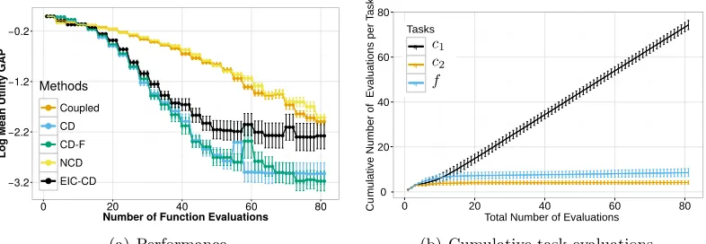
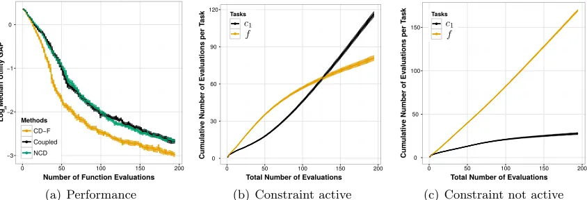
2. We analyze PESC in the decoupled scenario. We evaluate the accuracy of PESC when the different functions (objective or constraint) are evaluated independently. We show how PESC efficiently solves decoupled problems with an objective and constraints that compete for the same computational resource.
3. We intelligently balance the computational overhead of the Bayesian optimization method relative to the cost of evaluating the black-boxes. To achieve this, we develop a partial update to the PESC approximation that is less accurate but faster to compute. We then automatically switch between partial and full updates so that we can balance the amount of time spent in the Bayesian optimization subroutines and in the actual collection of data. This allows us to efficiently solve problems with a mix of decoupled functions where some are fast and others slow to evaluate.
The rest of the paper is structured as follows. Section 2 reviews prior work on constrained BO and considers these methods in the context of decoupled functions. In Section 3 we present a general framework for describing BO problems with decoupled functions, which contains as special cases the standard coupled framework considered in most prior work as well as the notion of decoupling introduced by Gelbart et al. (2014). This section also describes a general algorithm for BO problems with decoupled functions. In Section 4 we show how to extend Predictive Entropy Search (PES) (Hern´andez-Lobato et al., 2014) to solve Eq. (1) in the context of decoupling, an approach that we call Predictive Entropy Search with Constraints (PESC). We also show how PESC can be used to implement the general algorithm from Section 3. In Section 5 we modify the PESC algorithm to be more efficient in terms of wall-clock time by adaptively using an approximate but faster version of the method. In Sections 6 and 7 we perform empirical evaluations of PESC on coupled and decoupled optimization problems, respectively. Finally, we conclude in Section 8.
2. Related Work
Below we discuss previous approaches to Bayesian optimization with black-box constraints, many of which are variants of the expected improvement (EI) heuristic (Jones et al., 1998). In the unconstrained setting, EI measures the expected amount by which observing the objectivef atxleads to improvement over the current best recommendation orincumbent, the objective value of which is denoted by η (thus, η has the units of f, not x). The incumbent η is usually defined as the lowest expected value for the objective over the optimization domain. The EI acquisition function is then given by
αEI(x) =
Z
max(0, η−f(x))p(f(x)|D)df(x) =σf(x) (zf(x)Φ (zf(x)) +φ(zf(x))) , (2)
whereDrepresents the collected data (previous function evaluations) and p(f(x)|D) is the predictive distribution for the objective made by a Gaussian process (GP),µf(x) andσf2(x) are the GP predictive mean and variance for f(x), zf(x)≡(η−µf(x))/σf(x), and Φ and
2.1 Expected Improvement with Constraints
An intuitive extension of EI in the presence of constraints is to define improvement as only occurring when the constraints are satisfied. Because we are uncertain about the values of the constraints, we must weight the original EI value by the probability of the constraints being satisfied. This results in what we call Expected Improvement with Constraints (EIC):
αEIC(x) =αEI(x)
K Y k=1
Pr(ck(x)≥0|D) =αEI(x) K Y k=1
Φ
µk(x)
σk(x)
, (3)
The constraint satisfaction probability factorizes because f and c1, . . . , cK are modeled by independent GPs. In this expression µk and σk2 are the posterior predictive mean and variance for ck(x). EIC was initially proposed by Schonlau et al. (1998) and has been revisited by Parr (2013), Snoek (2013), Gardner et al. (2014) and Gelbart et al. (2014).
In the constrained setting, the incumbent η can be defined as the minimum expected objective value subject to all the constraints being satisfied at the corresponding location. However, we can never guarantee that all the constraints will be satisfied when they are only observed through noisy evaluations. To circumvent this problem, Gelbart et al. (2014) defineη as the lowest expected objective value subject to all the constraints being satisfied with posterior probability larger than the threshold 1−δ, where δ is a small number such as 0.05. However, this value for η still cannot be computed when there is no point in the search space that satisfies the constraints with posterior probability higher than 1−δ. For example, because of lack of data for the constraints. In this case, Gelbart et al. change the original acquisition function given by Eq. (3) and ignore the factorαEI(x) in that expression. This allows them to search only for a feasible location, ignoring the objectivef entirely and just optimizing the constraint satisfaction probability. However, this can lead to inefficient optimization in practice because the data collected for the objective f is not used to make optimal decisions.
2.2 Integrated Expected Conditional Improvement
Gramacy and Lee (2011) propose an acquisition function called the integrated expected conditional improvement (IECI), defined as
αIECI(x) =
Z X
αEI(x0)−αEI(x0|x)
h(x0)dx0. (4)
Here, αEI(x0) is the expected improvement at x0, αEI(x0|x) is the expected improvement atx0 given that the objective has been observed atx(but without making any assumptions about the observed value), and h(x0) is an arbitrary density over x0. The IECI at x is the expected reduction in EI at x0, under the density h(x0), caused by observing the objective atx. Gramacy and Lee use IECI for constrained BO by settingh(x0) to the probability of the constraints being satisfied at x0. They define the incumbent η as the lowest posterior mean for the objective f over the whole optimization domain, ignoring the fact that the lowest posterior mean for the objective may be achieved in an infeasible location.
values when the constraints are unlikely to be satisfied. This is not the case with IECI because Eq. (4) considers the EI over the whole optimization domain instead of focusing only on the EI at the current evaluation location, which may be infeasible with high probability. Gelbart et al. (2014) compare IECI with EIC for optimizing the hyper-parameters of a topic model with constraints on the entropy of the per-topic word distribution and show that EIC outperforms IECI on this problem.
2.3 Expected Volume Minimization
An alternative approach is given by Picheny (2014), who proposes to sequentially explore the location that most decreases the expected volume (EV) of the feasible region below the best feasible objective value η found so far. This quantity is computed by integrating the product of the probability of improvement and the probability of feasibility. That is,
αEV(x) =
Z
p[f(x0)≤η]h(x0)dx0−
Z
p[f(x0)≤min(η, f(x))]h(x0)dx0, (5)
where, as in IECI, h(x0) is the probability that the constraints are satisfied at x0. Picheny considers noiseless evaluations for the objective and constraint functions and defines η as the best feasible objective value seen so far or +∞when no feasible location has been found. A disadvantage of Picheny’s method is that it requires the integral in Eq. (5) to be computed over the entire search domain X, which is done numerically over a grid on x0. The resulting acquisition function must then be globally optimized. This is often performed by first evaluating the acquisition function on a grid onx. The best point in this second grid is then used as the starting point of a numerical optimizer for the acquisition function. This nesting of grid operations limits the application of this method to small input dimensionD. This is also the case for IECI whose acquisition function in Eq. (4) also includes an integral over X. Our method PESC requires a similar integral in the form of an expectation with respect to the posterior distribution of the global feasible minimizerx?. Nevertheless, this expectation can be efficiently approximated by averaging over samples ofx? drawn using the approach proposed by Hern´andez-Lobato et al. (2014). This approach is further described in Appendix B.3. Note that the integrals in Eq. (5) could in principle be also approximated by using Marcov chain Monte Carlo (MCMC) to sample from the unnormalized density
h(x0). However, this was not proposed by Picheny and he only described the grid based method.
2.4 Modeling an Augmented Lagrangian
Gramacy et al. (2016) propose to use a combination of EI and the augmented Lagrangian (AL) method: an algorithm which turns an optimization problem with constraints into a sequence of unconstrained optimization problems. Gramacy et al. use BO techniques based on EI to solve the unconstrained inner loop of the AL problem. When f and c1, . . . , cK are known the unconstrained AL objective is defined as
LA(x|λ1, . . . , λK, p) =f(x) +
K X k=1
1
2pmin(0, ck(x))
2−λ kck(x)
where p >0 is a penalty parameter and λ1 ≥0, . . . , λK ≥0 serve as Lagrange multipliers. The AL method iteratively minimizes Eq. (6) with different values for pand λ1, . . . , λK at each iteration. Letx(n)? be the minimizer of Eq. (6) at iterationnusing parameter valuesp(n)
and λ(n)1 , . . . , λ(n)K . The next parameter values are λk(n+1) = max(0, λ(n)k −ck(x
(n) ? )/p(n))
fork= 1, . . . , K andp(n+1) =p(n)ifx(n)
? is feasible andp(n+1) =p(n)/2 otherwise. Whenf
and c1, . . . , cK are unknown we cannot directly minimize Eq. (6). However, if we have
observations forf and c1, . . . , cK, we can then map such data into observations for the AL objective. Gramacy et al. fit a GP model to the AL observations and then select the next evaluation location using the EI heuristic. After collecting the data, the AL parameters are updated as above using the new values for the constraints and the whole process repeats.
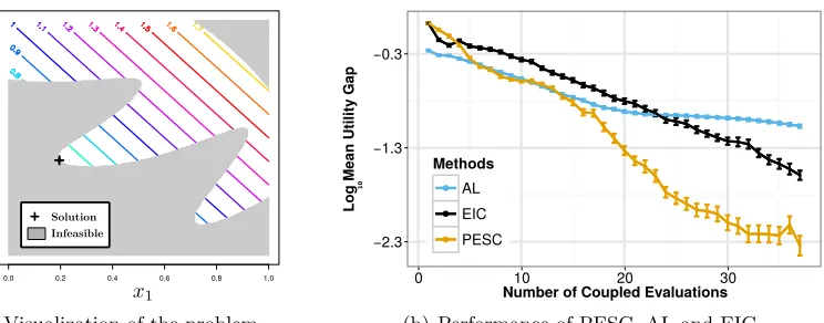
A disadvantage of this approach is that it assumes that the the constraintsc1, . . . , ckare noiseless to guarantee that that p and λ1, . . . , λK can be correctly updated. Furthermore, Gramacy et al. (2016) focus only on the case in which the objective f is known, although they provide suggestions for extending their method to unknownf. In section 6.3 we show that PESC and EIC perform better than the AL approach on the synthetic benchmark problem considered by Gramacy et al., even when the AL method has access to the true objective function and PESC and EIC do not.
2.5 Existing Methods for Decoupled Evaluations
The methods described above can be used to solve constrained BO problems with coupled
evaluations. These are problems in which all the functions (objective and constraints) are always evaluated jointly at the same input. Gelbart et al. (2014) consider extending the EIC method from Section 2.1 to thedecoupled setting, where the different functions can be independently evaluated at different input locations. However, they identify a problem with EIC in the decoupled scenario. In particular, the EIC utility function requires two conditions to produce positive values. First, the evaluation for the objective must achieve a lower value than the best feasible solution so far and, second, the evaluations for the constraints must produce non-negative values. When we evaluate only one function (objective or constraint), the conjunction of these two conditions cannot be satisfied by a single observation under a myopic search policy. Thus, the new evaluation location can never become the new incumbent and the EIC is zero everywhere. Therefore, standard EIC fails in the decoupled setting.
Gelbart et al. (2014) circumvent the problem mentioned above by treating decoupling as a special case and using a two-stage acquisition function: first, the next evaluation locationx
3. Decoupled Function Evaluations and Resource Allocation
We present a framework for describing constrained BO problems. We say that a set of functions (objective or constraints) are coupled when they always require joint evaluation at the same input location. We say that they are decoupled when they can be evaluated independently at different inputs. In practice, a particular problem may exhibit coupled or decoupled functions or a combination of both. An example of a problem with coupled functions is given by a financial simulator that generates many samples from the distribution of possible financial outcomes. If the objective function is the expected profit and the constraint is a maximum tolerable probability of default, then these two functions are computed jointly by the same simulation and are thus coupled to each other. An example of a problem with decoupled functions is the optimization of the predictive accuracy of a neural network speech recognition system subject to prediction time constraints. In this case different neural network architectures may produce different predictive accuracies and different prediction times. Assessing the prediction time may not require training the neural network and could be done using arbitrary network weights. Thus, we can evaluate the timing constraint without evaluating the accuracy objective.
When problems exhibit a combination of coupled and decoupled functions, we can then partition the different functions into subsets of functions that require coupled evaluation. We call these subsets of coupled functions tasks. In the financial simulator example, the objective and the constraint form the only task. In the speech recognition system there are two tasks, one for the objective and one for the constraint. Functions within different tasks are decoupled and can be evaluated independently. These tasks may or may not compete for a limited set of resources. For example, two tasks that both require the performance of expensive computations may have to compete for using a single available CPU. An example with no competition is given by two tasks, one which performs computations in a CPU and another one which performs computations in a GPU. Finally, two competitive tasks may also have different evaluation costs and this should be taken into account when deciding which one is going to be evaluated next.
artifi-cially coupling the tasks becomes increasingly inefficient as the cost differential is increased; for example, one might spend a week examining one aspect of a design that could have been ruled out within seconds by examining another aspect.
In the following sections we present a formalization of constrained Bayesian optimization problems that encompasses all of the cases described above. We then show that our method, PESC (Section 4), is an effective practical solution to these problems because it naturally separates the contributions of the different function evaluations in its acquisition function.
3.1 Competitive Versus Non-competitive Decoupling and Parallel BO
We divide the class of problems with decoupled functions into two sub-classes, which we
callcompetitive decoupling (CD) and non-competitive decoupling (NCD). CD is the form of
decoupling considered by Gelbart et al. (2014), in which two or more tasks compete for the same resource. This happens when there is only one CPU available and the optimization problem includes two tasks with each of them requiring a CPU to perform some expensive simulations. In contrast, NCD refers to the case in which tasks require the use of differ-ent resources and can therefore be evaluated independdiffer-ently, in parallel. This occurs, for example, when one of the two tasks uses a CPU and the other task uses a GPU.
Note that NCD is very related to parallel Bayesian optimization (see e.g., Ginsbourger et al., 2011; Snoek et al., 2012). In both parallel BO and NCD we perform multiple task evaluations concurrently, where each new evaluation location is selected optimally accord-ing to the available data and the locations of all the currently pendaccord-ing evaluations. The difference between parallel BO and NCD is that in NCD the tasks whose evaluations are currently pending may be different from the task that will be evaluated next, while in par-allel BO there is only a single task. Parpar-allel BO conveniently fits into the general framework described below.
3.2 Formalization of Constrained Bayesian Optimization Problems
We now present a framework for describing constrained BO problems of the form given by Eq. (1). Our framework can be used to represent general problems within any of the cate-gories previously described, including coupled and decoupled functions that may or may not compete for a limited number of resources, each of which may be replicated multiple times. LetF be the set of functions{f, c1, . . . , cK}and let the set of tasksT be a partition ofF in-dicating which functions are coupled and must be jointly evaluated. LetR={r1, . . . , r|R|} be the set of resources available to solve this problem. We encode the relationship be-tween tasks and resources with a bipartite graph G = (V,E) with vertices V =T ∪ R and edges {t∼r} ∈ E such that t ∈ T and r ∈ R. The interpretation of an edge {t ∼ r} is that task t can be performed on resource r. (We do not address the case in which a task requires multiple resources to be executed; we leave this as future work.) We also intro-duce acapacity ωmax for each resource r. The capacity ωmax(r)∈N represents how many
tasks resources functions
coupled objective
constraint
f
c1
t1 r1
non-competitive decoupled objective
constraint
f
c1
t1
t2 r2
r1
competitive decoupled objective
constraint
f
c1
t1
t2
r1
parallel
t1
r1
r2
objective
constraint
f
c1
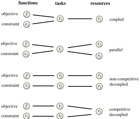
Figure 1: Schematic comparing the coupled, parallel, non-competitive decoupled (NCD), and competitive decoupled (CD) scenarios for a problem with a single constraint
c1. In each case, the mapping between tasks and resources (the right-hand portion of the figure) is the bipartite graphG.
We can now formally describe problems with coupled evaluations as well as NCD and CD. In particular, coupling occurs when two functionsg1 andg2 belong to the same task t. If this task can be evaluated on multiple resources (or one resource with ωmax > 1), then this is parallel Bayesian optimization. NCD occurs when two functions g1 and g2 belong to different tasks t1 and t2, which themselves require different resources r1 and r2, (that is, t1 ∼ r1, t2 ∼ r2 and r1 6= r2). CD occurs when two functions g1 and g2 belong to
different taskst1 andt2 (decoupled) that require thesame resource r (competitive). These
definitions are visually illustrated in Fig. 1. The definitions can be trivially extended to cases with more than two functions. The most general case is an arbitrary task-resource graphGencoding a combination of coupling, NCD, CD and parallel Bayesian optimization.
3.3 A General Algorithm for Constrained Bayesian Optimization
Algorithm 1 A general method for constrained Bayesian optimization.
1: Input: F,G= (T ∪ R,E),αt fort∈ T,X,M,D,ω,ωmax and δ.
2: repeat
3: for r∈ R such thatω(r)< ωmax(r) do 4: UpdateMwith any new data inD 5: fort∈ T such that {t∼r} ∈ E do 6: x∗t ←arg maxx∈Xαt(x|M)
7: α∗t ←αt(x∗t|M)
8: end for
9: t∗ ←arg maxt αt∗
10: Submit taskt∗ at input x∗t∗ to resource r 11: UpdateMwith the new pending evaluation 12: end for
13: untiltermination condition is met
14: Output: arg minx∈XEM[f(x)] s.t. p(c1(x)≥0, . . . , cK(x)≥0|M)≥1−δ
method PESC has this property, when the functions are modeled as independent. This property makes PESC an effective solution for the practical implementation of our general algorithm. By contrast, the EIC-D method of Gelbart et al. (2014) is not separable and cannot be applied in the general case presented here.
Algorithm 1 provides a general procedure for solving constrained Bayesian optimization problems. The inputs to the algorithm are the set of functions F, the set of tasks T, the set of resourcesR, the task-resource graph G= (T ∪ R,E), an acquisition function for each task, that is, αt for t ∈ T, the search space X, a Bayesian model M, the initial data set D, the resource query functionsω and ωmax and a confidence level δ for making a final recommendation. Recall that ωmax indicates how many tasks can be simultaneously executed on a particular resource. The functionω is introduced here to indicate how many tasks are currently being evaluated in a resource. The acquisition function αt measures the utility of evaluating taskt at the location x. This acquisition function depends on the predictions of the Bayesian modelM. The separability property of the original acquisition function guarantees that we can compute anαtfor each t∈ T.
Algorithm 1 works as follows. First, in line 3, we iterate over the resources, checking if they are available. Resource r is available if its number of currently running jobs ω(r) is less than its capacity ωmax(r). Whenever resource r is available, we check in line 4 if any new function observations have been collected. If this is the case, we then update the Bayesian model Mwith the new data (in most cases we will have new data since the resource r probably became available due to the completion of a previous task). Next, we iterate in line 5 over the tasks t that can be evaluated in the new available resource r
as dictated by G. In line 6 we find the evaluation location x∗
t that maximizes the utility obtained by the evaluation of task t, as indicated by the task-specific acquisition function
αt. In line 7 we obtain the corresponding maximum task utility α∗t. In line 9, we then maximize over tasks, selecting the taskt∗ with highest maximum task utilityα∗
t (this is the “competition” in CD). Upon doing so, the pair (t∗,x∗t∗) forms the next suggestion. This
(t,x) pairs in T × X that can be run on resource r. In line 10, we evaluate the selected task at resource r and in line 11 we update the Bayesian model M to take into account that we are expecting to collect data for taskt∗ at inputx∗t∗. This can be done for example
by drawing virtual data from M’s predictive distribution and then averaging across the predictions made when each virtual data point is assumed to be the data actually collected by the pending evaluation (Schonlau et al., 1998; Snoek et al., 2012). In line 13 the whole process repeats until a termination condition is met. Finally, in line 14, we give to the user a final recommendation of the solution to the optimization problem. This is the input that attains the lowest expected objective value subject to all the constraints being satisfied with posterior probability larger than 1−δ, where δ is maximum allowable probability of the recommendation being infeasible according to M.
Algorithm 1 can solve problems that exhibit any combination of coupling, parallelism, NCD, and CD.
3.4 Incorporating Cost Information
Algorithm 1 always selects, among a group of competitive tasks, the one whose evaluation produces the highest utility value. However, other cost factors may render the evaluation of one task more desirable than another. The most salient of these costs is the run time or duration of the task’s evaluation, which could depend on the evaluation location x. For example, in the neural network speech recognition system, one of the variables to be optimized may be the number of hidden units in the neural network. In this case, the run time of an evaluation of the predictive accuracy of the system is a function of xsince the training time for the network scales with its size. Snoek et al. (2012) consider this issue by automatically measuring the duration of function evaluations. They model the duration as a function ofxwith an additional Gaussian process (GP). Swersky et al. (2013) extend this concept over multiple optimization tasks so that an independent GP is used to model the unknown duration of each task. This approach can be applied in Algorithm 1 by penalizing the acquisition function for task twith the expected cost of evaluating that task. In particular, we can change lines 6 and 7 in Algorithm 1 to
6: x∗
t ←arg maxx∈Xαt(x|M)/ζt(x) 7: α∗
t ←αt(x∗t|M)/ζt(x∗t)
whereζt(x) is the expected cost associated with the evaluation of tasktatx, as estimated by a model of the collected cost data. When taking into account task costs modeled by Gaussian processes, the total number of GP models used by Algorithm 1 is equal to the number of functions in the constrained BO problem plus the number of tasks, that is, |F| +|T |. Alternatively, one could fix the cost functionsζt(x) a priori instead of learning them from collected data.
4. Predictive Entropy Search with Constraints (PESC)
Our acquisition function approximates the expected gain of information about the so-lution to the constrained optimization problem, which is denoted by x?. Importantly, our approximation is additive. For example, let A be a set of functions and let I(A) be the amount of information that we approximately gain in expectation by jointly evaluating the functions in A. Then I(A) =P
a∈AI({a}). Although our acquisition function is additive, the exact expected gain of information is not. Additivity is the result of a factorization assumption in our approximation (see Section 4.2 for further details). The good results obtained in our experiments seem to support that this is a reasonable assumption. Because of this additive property, we can compute an acquisition function for any possible subset
of f, c1, . . . , cK using the individual acquisition functions for these functions as building
blocks.
We follow MacKay (1992) and measure information aboutx?by the differential entropy ofp(x?|D), whereDis the data collected so far. The distributionp(x?|D) is formally defined in the unconstrained case by Hennig and Schuler (2012). In the constrained case p(x?|D) can be understood as the probability distribution determined by the following sampling process. First, we drawf,c1, . . . , cK from their posterior distributions givenDand second, we minimize the sampledf subject to the sampledc1, . . . , cK being non-negative, that is, we solve Eq. (1) for the sampled functions. The solution to Eq. (1) obtained by this procedure represents then a sample fromp(x?|D).
We consider first the case in which all the black-box functions f, c1, . . . , cK are evalu-ated at the same time (coupled). Let H [x?| D] denote the differential entropy of p(x?|D) and letyf,yc1, . . . , ycK denote the measurements obtained by querying the black-boxes for
f, c1, . . . , cK at the input location x. We encode these measurements in vector form as
y= (yf, yc1, . . . , ycK)
T. Note that y contains the result of the evaluation of all the func-tions at x, that is, the objective f and the constraints c1, . . . , cK. We aim to collect data at the location that maximizes the expected information gain or the expected reduction in the entropy ofp(x?|D). The corresponding acquisition function is
α(x) = H [x?| D]−Ey| D,x[H [x?| D ∪ {(x,y)}]] . (7)
In this expression, H [x?| D ∪ {(x,y)}] is the amount of information onx? that is available once we have collected new datayat the input locationx. However, this newyis unknown because it has not been collected yet. To circumvent this problem, we take the expectation with respect to the predictive distribution forygivenxandD. This produces an expression that does not depend ony and could in principle be readily computed.
A direct computation of Eq. (7) is challenging because it requires evaluating the entropy of the intractable distribution p(x?| D) when different pairs (x,y) are added to the data. To simplify computations, we note that Eq. (7) is the mutual information between x? and y given D and x, which we denote by MI(x?,y). The mutual information operator is symmetric, that is, MI(x?,y) = MI(y,x?). Therefore, we can follow Houlsby et al. (2012) and swap the random variables y and x? in Eq. (7). The result is a reformulation of the original equation that is now expressed in terms of entropies of predictive distributions, which are easier to approximate:
This is the same reformulation used by Predictive Entropy Search (PES) (Hern´andez-Lobato et al., 2014) for unconstrained Bayesian optimization, but extended to the case wherey is a vector rather than a scalar. Since we focus on constrained optimization problems, we call our method Predictive Entropy Search with Constraints (PESC). Eq. (8) is used by PESC to efficiently solve constrained Bayesian optimization problems with decoupled function evaluations. In the following section we describe how to obtain a computationally efficient approximation to Eq. (8). We also show that the resulting approximation is separable.
4.1 The PESC Acquisition Function
We assume that the functionsf,c1, . . . , cK are independent samples from Gaussian process (GP) priors and that the noisy measurements y returned by the black-boxes are obtained by adding Gaussian noise to the noise-free function evaluations atx. Under this Bayesian model for the data, the first term in Eq. (8) can be computed exactly. In particular,
H [y| D,x] = K+1
X i=1
1 2logσ
2 i(x) +
K+ 1
2 log(2πe), (9)
where σ2
i(x) is the predictive variance for yi atx and yi is the i-th entry in y. To obtain this formula we have used the fact that f, c1, . . . , cK are generated independently, so that H [y| D,x] = PK+1i=1 H [yi| D,x], and that p(yi| D,x) is Gaussian with variance parameter
σ2
i(x) given by the GP predictive variance (Rasmussen and Williams, 2006):
σ2
i(x) =ki(x)−ki(x)TK−1i ki(x) +νi, i= 1, . . . , K+ 1, (10)
where νi is the variance of the additive Gaussian noise in the i-th black-box, with f being the first one and cK the last one. The scalar ki(x) is the prior variance of the noise-free black-box evaluations at x. The vector ki(x) contains the prior covariances between the black-box values at xand at those locations for which data from the black-box is available. Finally, Ki is a matrix with the prior covariances for the noise-free black-box evaluations at those locations for which data is available.
The second term in Eq. (8), that is,Ex?| D[H [y| D,x,x?]], cannot be computed exactly
and needs to be approximated. We do this operation as follows. 1 : The expectation with respect top(x?| D) is approximated with an empirical average overM samples drawn from
p(x?| D). These samples are generated by following the approach proposed by Hern´ andez-Lobato et al. (2014) for samplingx? in the unconstrained case. We draw approximate pos-terior samples off, c1, . . . , cK, as described by Hern´andez-Lobato et al. (2014, Appendix A), and then solve Eq. (1) to obtainx? given the sampled functions. More details can be found in Appendix B.3 of this document. Note that this approach only applies for stationary kernels, but this class includes popular choices such as the squared exponential and Mat´ern kernels. 2 : We assume that the components of y are independent given D, x and x?, that is, we assume that the evaluations of f,c1, . . . , cK atx are independent given D and x?. This factorization assumption guarantees that the acquisition function used by PESC is additive across the different functions that are being evaluated. 3 : Let xj? be thej-th sample fromp(x?| D). We then find a Gaussian approximation to eachp(yi| D,x,xj?) using expectation propagation (EP) (Minka, 2001a). Letσ2
i(x|x j
approximation top(yi| D,x,xj?) given by EP. Then, we obtain
Ex?| D[H [y| D,x,x?]]
1
≈ 1
M
M X j=1
H
y| D,x,xj ?
2
≈ 1
M
M X j=1
"K+1 X i=1
H
yi| D,x,xj?
#
3
≈
K+1 X i=1
1
M
M X j=1 1 2logσ
2 i(x|xj?)
+ K+ 1
2 log(2πe), (11)
where each of the approximations has been numbered with the corresponding step from the description above. Note that in step 3 of Eq. (11) we have swapped the sums overiand j. The acquisition function used by PESC is then given by the difference between Eq. (9) and the approximation shown in the last line of Eq. (11). In particular, we obtain
αPESC(x) =
K+1 X i=1
˜
αi(x), (12)
where
˜
αi(x) =
1
M
M X j=1
1 2logσ
2 i(x)−
1 2logσ
2 i(x|xj?)
| {z }
˜
αi(x|xj?)
, i= 1, . . . , K+ 1. (13)
Interestingly, the factorization assumption that we made in step 2 of Eq. (11) has produced an acquisition function in Eq. (12) that is the sum of K+ 1 function-specific acquisition functions, given by the ˜αi(x) in Eq. (13). Each ˜αi(x) measures how much information we gain on average by only evaluating the i-th black box, where the first black-box evaluates
f and the last one evaluates cK+1. Furthermore, ˜αi(x) is the empirical average of ˜αi(x|x?) across M samples from p(x?|D). Therefore, we can interpret each ˜αi(x|x?) in Eq. (13) as a function-specific acquisition function conditioned on x?. Crucially, by using bits of information about the minimizer as a common unit of measurement, our acquisition function can make meaningful comparisons between the usefulness of evaluating the objective and constraints.
We now show how PESC can be used to obtain the task-specific acquisition functions required by the general algorithm from Section 3.3. Let us assume that we plan to evaluate only a subset of the functions f,c1, . . . , cK and let t⊆ {1, . . . , K + 1} contain the indices of the functions to be evaluated, where the first function is f and the last one is cK. We assume that the functions indexed by t are coupled and require joint evaluation. In this casetencodes atask according to the definition from Section 3.2. We can then approximate the expected gain of information that is obtained by evaluating this task at input x. The process is similar to the one used above when all the black-boxes are evaluated at the same time. However, instead of working with the full vectory, we now work with the components of y indexed by t. One can then show that the expected information gain obtained after evaluating task tat input xcan be approximated as
αt(x) =
X i∈t
˜
0.0 0.2 0.4 0.6 0.8 1.0 -2 -1 0 1 2
A) Sample fromp(f|D)
x f ( x ) x1 ?
0.0 0.2 0.4 0.6 0.8 1.0
-2
-1
0
1
2
B) Distributionp(y1|D,x)
x
y1
x1
?
0.0 0.2 0.4 0.6 0.8 1.0
-2
-1
0
1
2
C) Approx.p(y1|D,x,x1?)
x
y1
x1
?
0.0 0.2 0.4 0.6 0.8 1.0
0.0 0.2 0.4 0.6 0.8 1.0 1.2
D) Functionα˜1(x|x1?)
x ˜α1 ( x | x
1)?
x1
?
0.0 0.2 0.4 0.6 0.8 1.0
0.0 0.2 0.4 0.6 0.8 1.0 1.2
E) Functionα˜1(x)
x ˜α1 ( x ) x1 ?
0.0 0.2 0.4 0.6 0.8 1.0
-2
-1
0
1
2
F) Sample fromp(c1|D)
x c1 ( x ) x1 ?
0.0 0.2 0.4 0.6 0.8 1.0
-2
-1
0
1
2
G) Distributionp(y2|D,x)
x c1 ( x ) x1 ?
0.0 0.2 0.4 0.6 0.8 1.0
-2
-1
0
1
2
H) Approx.p(y2|D,x,x1?)
x c1 ( x ) x1 ?
0.0 0.2 0.4 0.6 0.8 1.0
0.0 0.2 0.4 0.6 0.8 1.0 1.2
I) Functionα˜2(x|x1?)
x ˜α2 ( x | x
1)?
x1
?
0.0 0.2 0.4 0.6 0.8 1.0
0.0 0.2 0.4 0.6 0.8 1.0 1.2
J) Functionα˜2(x)
x ˜α2 ( x ) x1 ?
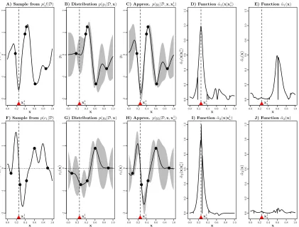
Figure 2: Illustration of the process followed to compute the function-specific acquisition functions given by Eq. (13). See the main text for details.
where the ˜αi are given by Eq. (13). PESC’s acquisition function is therefore separable since Eq. (14) can be used to obtain an acquisition function for each possible task. The process for constructing these task-specific acquisition functions is also efficient since it requires only to use the individual acquisition functions from Eq. (13) as building blocks. These two properties make PESC an effective solution for the practical implementation of the general algorithm from Section 3.3.
Fig. 2 illustrates with a toy example the process for computing the function-specific acquisition functions from Eq. (13). In this example there is only one constraint function. Therefore, the functions in the optimization problem are only f and c1. The search space
X is the unit interval [0,1] and we have collected four measurements for each function. The data for f are shown as black points in panels A, B and C. The data for c1 are shown as black points in panels F, G and H. We assume that f and c1 are independently sampled from a GP with zero mean function and squared exponential covariance function with unit amplitude and length-scale 0.07. The noise variance for the black-boxes that evaluate f
y2, that is, p(y1|D,x) and p(y2|D,x). Panels B and G show the means of these distribu-tions with confidence bands equal to one standard deviation. The first step to compute the ˜αi(x) from Eq. (13) is to draw M samples from p(x?|D). To generate each of these samples, we first approximately sample f and c1 from their posterior distributions p(f|D) and p(c1|D) using the method described by Hern´andez-Lobato et al. (2014, Appendix A). Panels A and F show one of the samples obtained for f and c1, respectively. We then solve the optimization problem given by Eq. (1) whenf andc1 are known and equal to the samples obtained. The solution to this problem is the input that minimizes f subject toc1 being positive. This produces a samplex1
? fromp(x?|D) which is shown as a discontinuous vertical line with a red triangle in all the panels. The next step is to find a Gaussian ap-proximation to the predictive distributions when we condition tox1
?, that is, p(y1|D,x,x1?) andp(y2|D,x,x1?). This step is performed using expectation propagation (EP) as described in Section 4.2 and Appendix A. Panels C and H show the approximations produced by EP for p(y1|D,x,x1?) and p(y2|D,x,x1?), respectively. Panel C shows that conditioning to x1? decreases the posterior mean of y1 in the neighborhood of x1?. The reason for this is that x1
? must be the global feasible solution and this means that f(x1?) must be lower than any other feasible point. Panel H shows that conditioning tox1
? increases the posterior mean of
y2 in the neighborhood of x1?. The reason for this is thatc1(x1?) must be positive because x1
? has to be feasible. In particular, by conditioning to x1? we are giving zero probability to all c1 such that c1(x1?)<0. Letσ12(x|x1?) and σ22(x|x1?) be the variances of the Gaussian approximations top(y1|D,x,x1?) andp(y2|D,x,x1?) and letσ12(x) andσ22(x) be the variances of p(y1|D,x) andp(y2|D,x). We use these quantities to obtain ˜α1(x|x1?) and ˜α2(x|x1?) ac-cording to Eq. (13). These two functions are shown in panels D and I. The whole process is repeatedM = 50 times and the resulting ˜α1(x|xj?) and ˜α2(x|xj?),j= 1, . . . , M, are averaged according to Eq. (13) to obtain the function-specific acquisition functions ˜α1(x) and ˜α2(x), whose plots are shown in panels E and J. These plots indicate that evaluating the objective
f is in this case more informative than evaluating the constraint c1. But this is certainly not always the case, as will be demonstrated in the experiments later on.
4.2 How to Compute the Gaussian Approximation to p(yi|D,x,xj?)
We briefly describe the process followed to find a Gaussian approximation to p(yi|D,x,xj?) using expectation propagation (EP) (Minka, 2001b). Recall that the variance of this ap-proximation, that is, σ2
i(x|x j
?), is used to compute ˜αi(x|xj?) in Eq. (13). Here we only provide a sketch of the process; full details can be found in Appendix A.
We start by assuming that the search space has finite size, that is, X ={x˜1, . . . ,x˜|X |}. In this case the functions f, c1, . . . , cK are encoded as finite dimensional vectors denoted
by f,c1, . . . ,cK. Thei-th entries in these vectors are the result of evaluatingf,c1, . . . , cK
at the i-th element of X, that is,f(˜x),c1(˜xi), . . . , cK(˜xi). Let us assume thatxj? andxare inX. Thenp(y|D,x,xj?) can be defined by the following rejection sampling process. First, we sample f, c1, . . . ,cK from their posterior distribution given the assumed GP models. We then solve the optimization problem given by Eq. (1). For this, we find the entry of f with lowest value subject to the corresponding entries of c1, . . . ,cK being positive.
Let i ∈ {1, . . . ,|X |} be the index of the selected entry. Then, if xj? 6= ˜xi, we reject the
indexed byx, that is, f(x), c1(x), . . . , cK(x) and then obtain yby adding to each of these values a Gaussian random variable with zero mean and varianceν1, . . . , νK+1, respectively. The probability distribution implied by this rejection sampling process can be obtained by first multiplying the posterior for f,c1, . . . ,cK with indicator functions that take value zero when f, c1, . . . ,cK should be rejected and one otherwise. We can then multiply the resulting quantity by the likelihood for y given f, c1, . . . ,cK. The desired distribution is finally obtained by marginalizing outf,c1, . . . ,cK.
We introduce several indicator functions to implement the approach described above. The first one Γ(x) takes value one whenx is a feasible solution and value zero otherwise, that is,
Γ(x) = K Y k=1
Θ[ck(x)], (15)
where Θ[·] is the Heaviside step function which is equal to one if its input is non-negative and zero otherwise. The second indicator function Ψ(x) takes value zero if x is a better solution than xj? according to the sampled functions. Otherwise Ψ(x) takes value one. In particular,
Ψ(x) = Γ(x)Θ[f(x)−f(xj?)] + (1−Γ(x)). (16)
Whenxis infeasible, this expression takes value one. In this case,xis not a better solution than xj? (because x is infeasible) and we do not have to reject. When x is feasible, the factor Θ[f(x)−f(xj?)] in Eq. (16) is zero whenxtakes lower objective value thanxj?. This will allow us to rejectf,c1, . . . ,cK whenxis a better solution thanxj?. Using Eq. (15) and Eq. (16), we can then writep(y|D,x,xj?) as
p(y|D,x,xj?)∝R p(y|f,c1, . . . ,cK,x)p(f,c1, . . . ,cK|D)Γ(xj?)
( Y
x0∈X
Ψ(x0)
)
| {z }
f(f,c1, . . . ,cK|xj?)
dfdc1· · ·cK, (17)
wherep(f,c1, . . . ,cK|D) is the GP posterior distribution for the noise-free evaluations of f,
c1, . . . , cK atX and p(y|f,c1, . . . ,cK,x) is the likelihood function, that is, the distribution
of the noisy evaluations produced by the black-boxes with input xgiven the true function values:
p(y|f,c1, . . . ,cK,x) =N(y1|f(x), ν1)N(y2|c1(x), ν2)· · · N(yK+1|cK(x), νK+1). (18)
The product of the indicator functions Γ and Ψ in Eq. (17) takes value zero whenever xj? is not the best feasible solution according to f,c1, . . . ,cK. The indicator Γ in Eq. (17) guarantees that xj? is a feasible location. The product of all the Ψ in Eq. (17) guarantees that no other point in X is better than xj?. Therefore, the product of Γ and the Ψ in Eq. (17) rejects any value of f,c1, . . . ,cK for which xj? is not the optimal solution to the constrained optimization problem.
have a closed form solution because of the complexity introduced by the the product of indicator functions Γ and Ψ. This means that Eq. (17) cannot be exactly computed and has to be approximated. For this, we use EP to fit a Gaussian approximation to the product
ofp(f,c1, . . . ,cK|D) and the indicator functions Γ and Ψ in Eq. (17), which we have denoted
by f(f,c1, . . . ,cK|xj?), with a tractable Gaussian distribution given by
q(f,c1, . . . ,cK|x?j) =N(f|m1,V1)N(c1|m2,V2)· · · N(cK|mK+1,VK+1), (19)
where m1, . . . ,mK+1 and V1, . . . ,VK+1 are mean vectors and covariance matrices to be determined by the execution of EP. Letvi(x) be the diagonal entry ofVi corresponding to the evaluation location given byx, wherei= 1, . . . , K+ 1. Similarly, letmi(x) be the entry of mi corresponding to the evaluation location xfor i= 1, . . . , K+ 1. Then, by replacing
f(f,c1, . . . ,cK|xj?) in Eq. (17) with q(f,c1, . . . ,cK|xj?), we obtain
p(y|D,x,xj
?)≈ K+1
Y i=1
N(yi|mi(x), vi(x) +νi). (20)
Consequently, σ2 i(x|x
j
?) =vi(x) +νi can be used to compute ˜αi(x|xj?) in Eq. (13).
The previous approach does not work when the search space X has infinite size, for example whenX = [0,1]d withdbeing the dimension of the inputs tof, c
1, . . . , cK. In this
case the product of indicators in Eq. (17) includes an infinite number of factors Ψ(x0), one for each possible x0 ∈ X. To solve this problem we perform an additional approximation. For the computation of Eq. (17), we consider thatX is well approximated by the finite set
Z, which contains only the locations at which the objective f has been evaluated so far, the value ofxj? andx. Therefore, we approximate the factor Qx0∈XΨ(x0) in Eq. (17) with
the factorQ
x0∈ZΨ(x0), which has now finite size. We expect this approximation to become
more and more accurate as we increase the amount of data collected for f. Note that our approximation to X is finite, but it is also different for each location x at which we want to evaluate Eq. (17) sinceZ is defined to containx. A detailed description of the resulting EP algorithm, indicating how to compute the variance functions vi(x) shown in Eq. (20), is given in Appendix A.
The EP approximation to Eq. (20), performed after replacing X with Z, depends on the values of D,xj? and x. Having to re-run EP for each value ofx at which we may want to evaluate the acquisition function given by Eq. (12) is a very expensive operation. To avoid this, we split the EP computations between those that depend only on D and xj?, which are the most expensive ones, and those that depend only on the value of x. We perform the former computations only once and then reuse them for each different value of
x. This allows us to evaluate the EP approximation to Eq. (17) at different values of xin a computationally efficient way. See Appendix A for further details.
4.3 Efficient Marginalization of the Model Hyper-parameters
hyper-parameters under some non-informative prior. Ideally, we should then average the GP predictive distributions with respect to the generated samples before approximating the information gain. However, this approach is too computationally expensive in practice. Instead, we follow Snoek et al. (2012) and average the PESC acquisition function with respect to the generated hyper-parameter samples. In our case, this involves marginalizing each of the function-specific acquisition functions from Eq. (13). For this, we follow the method proposed by Hern´andez-Lobato et al. (2014) to average the acquisition function of Predictive Entropy Search in the unconstrained case. Let Θ denote the model hyper-parameters. First, we draw M samples Θ1, . . . ,ΘM from the posterior distribution of Θ given the data D. Typically, for each of the posterior samples Θj of Θ we draw a single corresponding sample xj? from the posterior distribution of x? given Θj, that is,
p(x?| D,Θj). Let σ2i(x|Θj) be the variance of the GP predictive distribution for yi when the hyper-parameter values are fixed toΘj, that is,p(y
i|D,x,Θj), and letσi2(x|xj?,Θj) be the variance of the Gaussian approximation to the predictive distribution for yi when we condition to the solution of the optimization problem being xj? and the hyper-parameter values being Θj. Then, the version of Eq. (13) that marginalizes out the model hyper-parameters is given by
˜
αi(x) =
1
M
M X j=1
1 2logσ
2
i(x|Θj)− 1 2logσ
2
i(x|xj?,Θj)
, i= 1, . . . , K+ 1. (21)
Note that j is now an index over joint posterior samples of the model hyper-parametersΘ
and the constrained minimizerx?. Therefore, we can marginalize out the hyper-parameter values without adding any additional computational complexity to our method because a loop over M samples of x? is just replaced with a loop over M joint samples of (Θ,x?). This is a consequence of our reformulation of Eq. (7) into Eq. (8). By contrast, other techniques that work by approximating the original form of the acquisition function used in Eq. (7) do not have this property. An example in the unconstrained setting is Entropy Search (Hennig and Schuler, 2012), which requires re-computing an approximation to the acquisition function for each hyper-parameter sampleΘj.
4.4 Computational Complexity
In the coupled setting, the complexity of PESC is O(M KN3), where M is the number of posterior samples of the global constrained minimizer x?, K is the number of constraints, andN is the number of collected data points. This cost is determined by the cost of each EP iteration, which requires computing the inverse of the covariance matricesV1, . . . ,VK+1 in Eq. (20). The dimensionality of each of these matrices grows with the size of Z, which is determined by the numberN of objective evaluations (see the last paragraph of Section 4.2). Therefore each EP iteration has cost O(KN3) and we have to run an instance of EP for each of the M samples of x?. If M is also the number of posterior samples for the GP hyperparameters, as explained in Section 4.3, this is the same computational complexity as in EIC. However, in practice PESC is slower than EIC because of the cost of running multiple iterations of the EP algorithm.
k−1. The origin of this cost is again the size of the matrices V1, . . . ,VK+1 in Eq. (20). WhileV1still scales as a function of|Z|, we have thatV2, . . . ,VK+1 scale now as a function of|Z|plus the number of observations for the corresponding constraint function. The reason for this is thatQ
x0∈ZΨ(x0) is used to approximateQx0∈XΨ(x0) in Eq. (17) and each factor
inQ
x0∈ZΨ(x0) represents then a virtual data point for each GP. See Appendix A for details.
The cost of sampling the GP hyper-parameters is O(M KN3) and therefore, it does not affect the overall computational complexity of PESC.
4.5 Relationship between PESC and PES
PESC can be applied to unconstrained optimization problems. For this we only have to set
K = 0 and ignore the constraints. The resulting technique is very similar to the method PES proposed by Hern´andez-Lobato et al. (2014) as an information-based approach for unconstrained Bayesian optimization. However, PESC without constraints and PES are not identical. PES approximatesp(y|D,x,xj?) by multiplying the GP predictive distribution by additional factors that enforce xj? to be the location with lowest objective value. These factors guarantee that 1) the value of the objective at xj? is lower than the minimum of the values for the objective collected so far, 2) the gradient of the objective is zero at x? and 3) the Hessian of the objective is positive definite at x?. We do not enforce the last two conditions since the global optimum may be on the boundary of a feasible region and thus conditions 2) and 3) do not necessarily hold (this issue also arises in PES because the optimum may be on the boundary of the search space X). Condition 1) is implemented in PES by taking the minimum observed value for the objective, denoted by η, and then imposing the soft condition f(xj?) < η+, where ∼ N(0, ν) accounts for the additive Gaussian noise with varianceν in the black-box that evaluates the objective. In PESC this is achieved in a more principled way by using the indicator functions given by Eq. (16).
4.6 Summary of the Approximations Made in PESC
We describe here all the approximations performed in the practical implementation of PESC. PESC approximates the expected reduction in the posterior entropy ofx? (see Eq. 7) with the acquisition function given by Eq. (12). This involves the following approximations:
1. The expectation over x? in Eq. (8) is approximated with Monte Carlo sampling.
2. The Monte Carlo samples of x? come from samples of f, c1, . . . , cK drawn approxi-mately using a finite basis function approximation to the GP covariance function, as described by Hern´andez-Lobato et al. (2014, Appendix A).
3. We approximate the factor Q
x0∈XΨ(x0) in Eq. (17) with the factor
Q
x0∈ZΨ(x0).
Unlike the original search spaceX,Zhas now finite size and the corresponding product of Ψ indicators is easier to approximate. The setZ is formed by the locations of the current observations for the objective f and the current evaluation location xof the acquisition function.
4. After replacing Q
x0∈XΨ(x0) with
Q
x0∈ZΨ(x0) in Eq. (17), we further approximate
by the right-hand-side of Eq. (20). We use the method expectation propagation (EP) for this task, as described in Appendix A. Because the EP approximation in Eq. (19) factorizes acrossf,c1, . . . ,cK, the execution of EP implicitly includes the factorization assumption performed in step 2 of Eq. (11).
5. As described in the last paragraph of Section 4.2, in the execution of EP we separate the computations that depend onDandxj?, which are very expensive, from those that depend on the location x at which the PESC acquisition function will be evaluated. This allows us to evaluate the approximation to Eq. (17) at different values ofx in a computationally efficient way.
6. To deal with unknown hyper-parameter values, we marginalize the acquisition function over posterior samples of the hyper-parameters. Ideally, we should instead marginalize the predictive distributions with respect to the hyper-parameters before computing the entropy, but this is too computationally expensive in practice.
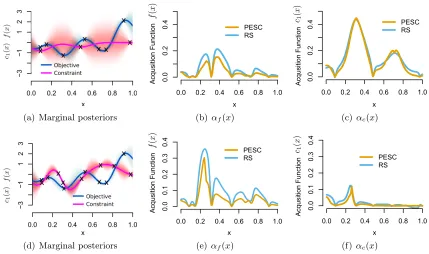
In Section 6.1, we assess the accuracy of these approximations (except the last one) and show that PESC performs on par with a ground-truth method based on rejection sampling. Note that in addition to the mathematical approximations described above, additional sources of error are introduced by the numerical computations involved. In addition to the usual roundoff error, etc., we draw the reader’s attention to the fact that the x? samples are the result of numerical global optimization of the approximately drawn samples of
f, c1, . . . , cK, and then the suggestion is chosen by another numerical global optimization
of the acquisition function. At present, we do not have guarantees that the true global optimum is found by our numerical methods in each case.
5. PESC-F: Speeding Up the BO Computations
decide when to switch between the slow and the fast versions of those computations. In the following paragraphs we address these issues.
We propose ways to reduce the cost of the computations performed by PESC after collecting each new data point. These computations include
1. Drawing posterior samples of the GP hyper-parameters and then for each sample computing the Cholesky decomposition of the kernel matrix.
2. Drawing approximate posterior samples ofx? and then running an EP algorithm for each of these samples.
3. Globally maximizing the resulting acquisition functions.
We shorten each of these steps. First, we reduce the cost of step 1 by skipping the sampling of the GP hyper-parameters and instead considering the hyper-parameter samples already used at an earlier iteration. This also allows for additional speedups by using fast (O(N2)) updates of the Cholesky decomposition of the kernel matrix instead of recomputing it from scratch. Second, we shorten step 2 by skipping the sampling ofx? and instead considering the samples used at the previous iteration. We also reuse the EP solutions computed at the previous iteration (see Appendix A for further details on how to reuse the EP solutions). Finally, we shorten step 3 by using a coarser termination condition tolerance when maxi-mizing the acquisition function. This allows the optimization process to converge faster but with reduced precision. Furthermore, if the acquisition function is maximized using a local optimizer with random restarts and/or a grid initialization, we can shorten the computation further by reducing the number of restarts and/or grid size.
5.1 Choosing When to Run the Fast or the Slow Version
The motivation for PESC-F is that the time spent in the BO computations should be small compared to the time spent evaluating the black-box functions. Therefore, our approach is to switch between two distinct types of BO computations: the full (slow) and the partial (fast) PESC computations. Our goal is to approximately keep constant the fraction of total wall-clock time consumed by such computations. To achieve this, at each iteration of the BO process, we use the slow version of the computations if and only if
τnow−τlast
τslow
> γ , (22)
where τnow is the current time, τlast is the time at which the last slow BO computations were complete,τslow is the duration of the last execution of the slow BO computations (this includes the time passed since the actual collection of the data until the maximization of the acquisition function) and γ > 0 is a constant called the rationality level. The larger the value of γ, the larger the amount of time spent in rational decision making, that is, in performing BO computations. Algorithm 2 shows the steps taken by PESC-F for the decoupled competitive case. In this case each function f, c1, . . . , cK represents a different task, that is, the different functions can be evaluated in a decoupled manner and in addition to this, all of them compete for using a single computational resource.
Algorithm 2 PESC-F for competitive decoupled functions.
1: Inputs: T ={{f},{c1}, . . . ,{cK}},D,γ,δ.
2: τlast←0
3: τslow←0
4: repeat
5: τnow ←current time
6: if (τnow−τlast)/τslow> γ then
7: Sample GP hyper-parameters
8: Fit GP toD
9: Generate new samples ofx?
10: Compute the EP solutions from scratch
11: τslow←current time−τnow
12: τlast←current time
13: {x∗, t∗} ←arg maxx∈X,t∈T αt(x) (expensive optimization)
14: else
15: Update fit of GP toD 16: Reuse previous EP solutions
17: {x∗, t∗} ←arg maxx∈X,t∈T αt(x) (cheap optimization)
18: end if
19: Add to D the evaluation of the function in task t∗ at input x∗ 20: untiltermination condition is met
21: Output: arg minx∈XEGP[f(x)] s.t. p(c1(x)≥0, . . . , cK(x)≥0|GP)≥1−δ
slow update since these durations may exhibit deterministic trends. For example, the cost of computations tends to increase at each iteration due to the increase in data set size. If indeed the update duration increases monotonically, then the duration of the most recent update would be a more accurate estimate of the duration of the next slow update than the average duration of all past updates.
PESC-F can be used as a generalization of PESC, since it reduces to PESC in the case of sufficiently slow function evaluations. To see this, note that the time spent in a function evaluation will be upper bounded by τnow−τlast and according to Eq. (22), the slow computations are performed whenτnow−τlast> γτslow. When the function evaluation takes a very large amount of time, we have thatτslowwill always be smaller than that amount of time and the conditionτnow−τlast> γτslowwill always be satisfied for reasonable choices of γ. Thus, PESC-F will always perform slow computations as we would expect. On the other hand, if the evaluation of the black-box function is very fast, PESC-F will mainly perform fast computations but will still occasionally perform slow ones, with a frequency roughly proportional to the function evaluation duration.
5.2 Setting the Rationality Level in PESC-F
correspond to spending roughly 50−90% of the total time performing function evaluations. The optimalγ may also change at different stages of the BO process. Selecting the optimal value ofγ is a subject for future research. Note that in PESC-F we are making sub-optimal decisions because of time constraints. Therefore, PESC-F is a simple example of bounded
rationality, which has its roots in the traditional AI literature. For example, Russell (1991)
proposes to treat computation as a possible action that consumes time but increases the expected utility of future actions.
5.3 Bridging the Gap Between Fast and Slow Computations
As discussed above, PESC-F can be applied even when function evaluations are very slow, as it automatically reverts to standard PESC when τeval > τslow. However, if the func-tion evaluafunc-tions are extremely fast, that is, faster even that the fast PESC updates, then even PESC-F violates the condition that the decision-making should take less time than the function evaluations. We have already defined τslow as the duration of the slow BO computations. Let us also defineτfastas the duration of the fast BO computations and τeval as the duration of the evaluation of the functions. Then, the intuition described above can be put into symbols by saying that PESC-F is most useful whenτfast < τeval< τslow.
Many aspects of PESC-F are not specific to PESC and could easily be adapted to other acquisition functions like EIC or even unconstrained acquisition functions like PES and EI. In particular, lines 9, 10 and 16 of Algorithm 2 are specific to PESC, whereas others are common to other techniques. For example, when using vanilla unconstrained EI, the computational bottleneck is likely to be the sampling of the GP hyper-parameters (Algorithm 2, line 7) and maximizing the acquisition function (Algorithm 2, line 13). The ideas presented above, namely to skip the hyper-parameter sampling and to optimize the acquisition function with a smaller grid and/or coarser tolerances, are applicable in this situation and might be useful in the case of a fairly fast objective function. However, as mentioned above, in the single-task case one retains the option to abandon BO entirely for a faster method, whereas in the multi-task case considered here, neither a purely slow nor a purely fast method suits the nature of the optimization problem. An interesting direction for future research is to further pursue this notion of optimization algorithms that bridge the gap between those designed for optimizing cheap (fast) functions and those designed for optimizing expensive (slow) functions.
6. Empirical Analyses in the Coupled Case
We first evaluate the performance of PESC in experiments with different types of coupled optimization problems. First, we consider synthetic problems of functions sampled from the GP prior distribution. Second, we consider analytic benchmark problems that were previ-ously used in the literature on Bayesian optimization with unknown constraints. Finally, we address the meta-optimization of machine learning algorithms with unknown constraints.