A Novel Clustering Algorithm and Its Incremental Version
for Large-Scale Text Collection
Lei Chen
Harbin Institute of Technology, School of Management, Harbin, 150001, China Beijing Normal University, Zhu Hai, International Business Faculty, 519087, China
e-mail: [email protected]
Ming Liu*
Harbin Institute of Technology, School of Computer Science and Technology, Harbin, 150001, China e-mail: [email protected]
Chong Wu
Harbin Institute of Technology, School of Management, Harbin, 150001, China e-mail: [email protected]
Ai Xu
Beijing Normal University, Zhu Hai, International Business Faculty, 519087, China e-mail: [email protected]
http://dx.doi.org/10.5755/j01.itc.45.2.8666
Abstract. Nowadays, the fast advance of internet technology has brought two challenges. One is the explosion of information. The other is that new information appears almost every day. Obviously, clustering is a good solution to help users analyze information automatically, whereas traditional clustering algorithms are only suitable for small- scale and stable text collection. In order to cluster large-scale and unstable texts, a novel clustering algorithm based on vector compression is proposed in this paper. We call this algorithm VCLC, abbreviated from a clustering algorithm based on vector compression for large-scale text collection. Experimental results demonstrate that VCLC is effective for clustering large-scale text collection. The reason is that VCLC selects related features to compress feature sets, and iterative training idea of self-organizing-mapping (SOM) is also adopted in it to fine-tune the weights of the features to enhance clustering performance. Besides, an incremental version of VCLC, namely I-VCLC, is also provided in this paper. When novel texts appear, I-VCLC chooses some samples from the original texts to alter neuron model to perform incremental clustering. In order to prevent over training, I-VCLC adjusts the weights of the samples along with training process. Experimental results demonstrate that I-VCLC can cluster unstable texts very well.
Keywords: vector compression; incremental clustering; self-organizing-mapping; neuron model.
1. Introduction
Along with the fast advance of internet technology, information overload has already become a headache problem to users. Obviously, clustering is a good solution to this issue. It partitions data into clusters and does not need any transcendent knowledge [1]. Due to the fact that text is a common descriptive
format to express information in website, it causes text clustering becomes hotter and hotter.
In comparison with the other types of data (e.g. figure, video, etc.), text vector is very sparse. That means the features that are related to the topic of text only occupy a small proportion of vector space. This problem is also called “curse of dimensionality” [2]. It causes similarities among most of texts are close to 0. This situation dramatically drops the performance of traditional clustering algorithms. The typical examples are Spectral Clustering [3], Graph Clustering [4], and Hybrid of K-means and KNN [5]. They all perform well on clustering dense data, such as figure and video, but fail in dealing with sparse data, such as text. In order to solve “curse of dimensionality”, Principal Component Analysis (PCA) [6] and Latent Semantic Indexing (LSI) [7] are adopted as preprocessing step to reduce vector dimension before clustering. But, since PCA and LSI combine several features together to construct a fake feature, the semantic meaning of the feature is also lost, which, somehow, drops the performance of clustering algorithms.
In fact, in text clustering, it only needs to choose small features from vector space to comprehensively represent the topic of one cluster. For example, if there is a cluster whose topic is about “military”, only the features, such as “gun”, “sword”, “tank”, which are related to the topic of the cluster can be chosen as the representation of this cluster.
Obviously, if only related features are chosen to represent cluster, it not only can filter the interferences brought from unrelated features, but also can reduce memory storage. For example, after word stemming and common word filtration, if we use Vector Space Model to organize the testingtexts in the experiments (those texts are downloaded from Yahoo web site during the entire year of 2014, including about 107
texts), the dimension of vector space exceeds 108.
That means it needs 200G memories to store this model. On the contrary, if we treat the representation of text and cluster as feature set, and only choose the words in the texts that are related to the topic of the cluster as features, it only needs 80M memories.
In order to cluster large-scale text collection effectively, a novel text clustering algorithm based on vector compression is proposed in this paper. We call this algorithm VCLC for simplicity. In our early paper [8], we also consider choosing features to reconstruct cluster vector. However, this reconstruction is based on two statistics (namely, intra-cluster agglomeration and inter-cluster distinctness), and two processes (reconstruction and clustering) run for two distinct objectives. In detail, the aim of reconstruction is to compress vector dimension and the aim of clustering is to cluster similar texts. The discrepancy between the two aims causes that the algorithm in [8] may not always converge to the best result. In experiments (Figure 11 and Figure 12), we compare the clustering result obtained by our algorithm (VCLC) proposed in this paper with the algorithm (VRCLC) proposed in our early paper [8]. Experimental results demonstrate that our algorithm (VCLC) outperforms the algorithm
(VRCLC) in [8] from both running time and clustering precision. The reason to this result is that VCLC adjusts the similar features to keep the semantically similar texts aggregate together. In detail, VCLC first chooses the features that are related to the topic of the cluster to represent cluster, and then iterative training idea of self-organizing-mapping (SOM) is adopted to fine-tune the weights of the chosen features to enhance clustering precision. Experimental results demonstrate that since related features are chosen to represent cluster, VCLC can remove the disturbances brought from useless features and thereby owns high intra-cluster agglomeration. Moreover, since only related features are put in feature set to represent cluster, the clusters represented by those feature sets express distinct meanings. That means the clusters formed by VCLC are also separated well.
Information on website is updated every moment. Therefore, how to cluster unstable textual data is also important [9~11]. To this end, this paper proposes an incremental version of VCLC (namely, I-VCLC). When novel texts appear, I-VCLC combines novel texts and some samples chosen from the original texts together to alter neuron model generated from the original texts to perform incremental clustering. In order to make the chosen samples better simulate the distribution of the original texts and furthermore to reduce running time, local density is used to partition neuron model into several regions to generate samples. Experimental results demonstrate that I-VCLC can cluster unstable textual data with low running time.
2. Clustering algorithm for large-scale text
collection (VCLC)
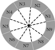
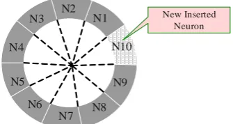
The core idea of VCLC is to choose the related and useful features from vector space to represent each cluster. After selection, one cluster is represented by one feature set containing the features related to the topic of the cluster. Iterative training idea of SOM is adopted to conduct training process. In this training process, one cluster is treated as one neuron, and all the neurons are ordered as round topology. Round topology is simple and can avoid “boundary problem” of square topology [12]. This topology is shown in Figure 1, and how to insert neuron in this topology is shown in Figure 2.
N1 N2 N3
N4
N5
N6 N7
N8 N9
N10 N1 N2 N3
N4
N5
N6
N7 N8
N9
New Inserted Neuron
Figure 2. Insert new neuron inround neuron topology
2.1. Initialization of VCLC
Traditional SOM based algorithms randomly initialize weights on features in neuron. That means each feature will be assigned an arbitrary weight at the beginning of training process. This way increases training time and does not consider any transcendental knowledge derived from input texts [13]. Thereby, this paper uses semantic similarity among features to form a more rational initial neuron mode. The neurons in this model represent the clusters of distinct topics.
In order to form initial neuron model, it needs to calculate semantic similarity among features at first. After that, features are partitioned into feature sets, and one feature set represents one neuron (or one cluster) in the initial neuron model. Because one feature set contains the features semantically similar to each other, it indicates that this initial neuron model can partition texts into different clusters each of which expresses the distinct topic to the others. The linguist indicates: “the syntax function of a feature is the distribution of this feature” [14].The context of one feature is a typical distribution. Therefore, if the contexts of two features are almost the same, the semantic similarity between these two features is close. The word before a feature and the word after a feature mostly determine the semantic meaning of this feature. Thus, we count feature’s co-occurring word and co-occurring word probability to construct feature’s co- occurring word vector. One dimensionality of this vector corresponds to one co-occurring word of one feature. The value of this dimensionality is the co-occurring word probability between the feature and its co-occurring word. Via calculating Kullback-Leibler divergence between two co-occurring word vectors of two features, semantic similarity between these two features can be obtained like
(
p,
q) 1-
(
,
)
Sim F F
H
FV F
(
p)
FV F
(
q)
(1)where Fp and Fq denote two features, and FV(Fp) and FV(Fq) denote the co-occurring word vectors of Fp
and Fq; H(FV(Fp),FV(Fq)) denotes the Kullback-Leibler divergence between two vectors. To calculate
H(FV(Fp),FV(Fq)), we need to acquire the value of each entry in FV(Fp) and FV(Fq) at first. This value represents the semantic similarity between one feature, e.g. Fp, and its one co-occurring word, e.g. CoWk [15].
It can be calculated by
, ,
(
)
(
)
(
)
(
)
p k
p k
p k
Co F CoW
P F CoW
Fre F
Fre CoW
(2)where Fp denotes one feature; CoWk denotes one
co-occurring word of Fp; Co(Fp,CoWk) denotes the
frequency of the concurrence of Fp and CoWk in the
texts.
Via Eq.(2), we can calculate the Kullback-Leibler divergence between two co-occurring word vectors, e.g. FV(Fp) and FV(Fq), as
2 1
2 2
1 1
( )
( , ) - log ( )
2
1
+ ( log ) ( log ) 2
n
i i
i i
i
n n
i i i i
i i
p q
H p q
p p q q
( p) ( q)
FV F FV F
(3)
where pidenotes ith entry in FV(Fp) and qi denotes ith
entry in FV(Fq). They can be calculated by Eq.(2). n denotes the size of the co-occurring word vector. From Eq.(3), it can be concluded that the Kullback-Leibler divergence ranges in [0, 1]. The larger is the difference between the contexts of two features, the bigger is the value of the Kullback-Leibler divergence. Thus, we can use Kullback-Leibler divergence to measure the semantic similarity between two features.
After obtaining semantic similarity among features, all the features in vector space can be partitioned into feature clusters by any clustering algorithm, and each cluster includes the features that are semantically similar to each other. Because it is unable to predict the amount of feature clusters, Hierarchical Clustering [16] is adopted by us to cluster features.
Via Hierarchical Clustering, one feature cluster is treated as one feature set used to represent one cluster. Since the features in one feature set are semantically similar, the clusters represented by this kind of feature sets are partitioned well. Besides, since only the semantically similar features are contained by feature set, that means compared with traditional vector representation that uses all the features in vector space to form cluster vector, our semantic initialization can dramatically reduce vector dimension. Unfortunately, the feature sets constructed by semantic initialization are coarse, thus we use iterative training process of SOM to fine-tune the feature sets to obtain better cluster partition. In order to conduct training process, we need to change the feature sets constructed by semantic initialization to an initial neuron model. For this purpose, we first treat one feature set as one neuron, and then randomly insert neurons to form a round topology as shown in Figure 1 and Figure 2.
2.2. Training process of VCLC
Input: initial neuron set N; text collection D; topology matrix SN; max tuning threshold tmax; stopping criteria s.
Output: neuron set (or cluster set) C.
Initialization:
/* Call function square( ) to set the topology of neuron model as square. */
SN=square( );
Tuning process:
/* Initialize tuning index as 0. */ t=0;
while (t<tmax) {
t=t+1;
/* Set d as a text variable and choose one text from D to set it. */
Doc d; d=random(D);
/* ne is a neuron variable. */ Neuron ne;
/* Calculate the similarity between d and each neuron in neuron topology by function callsim( ).*/
/* Function callsim( ) returns the neuron that has the max similarity to d. */
ne=callsim(d,N);
/* Use function adjust( ) to adjust neuron ne via d. */ ne=adjust(ne,d);
/* Sort the features in ne in order of their weights. */ ne=sort(ne);
/* Keep the features in ne whose weights are larger than the others in the number of limit and remove the other features. */
ne=featuretrim(ne);
/* Use function topology( ) to return the neurons that are adjacent with ne. */
Neuron tempN[ ]=topology(SN,ne); for (i=1;i<tempN[ ].length( );i++) {
tempN[i]=adjust(tempN[i],d);
/* Treat one neuron in N as one cluster in C. */ C=N;
}
/* Use function stopcal( ) to calculate the similarity between any neuron pair in N*/
float p=stopcal(N);
/* If it achieves criteria, stop running. */ if(p>s)
return C; }
In callsim(d,N), we need to calculate the similarity between one text and one neuron. Traditional SOM based algorithms [17,18] apply vector to represent neuron, and one entry in this vector corresponds to one feature in vector space. If we adopt this way too, many useless features will be contained in the vector and a lot of memory will be spent. Besides, in this situation, vector based similarity measurements, such as Euclidean distance, will spend much running time. In order to solve those problems, we apply feature set to represent neuron in this paper, and the features in one feature set are semantically similar to each other.
In order to use feature set to represent neuron, we need to adjust the similarity measurement in traditional SOM based algorithms as:
0; | | | ( ) | /3
( , ) ( , ) log(| |); ( , ) ( , ) ( , ) | k i k i k i FS k k i k i D F k i
f S N
i_
If FS D
W i_f D W i_f N W i_f D W i_f N S
FS D FS N FS D FS N
F im D N
If
k i | | ( k) | /3
S D FS N FS D
(4) where Dk denotes kth text in text collection; Ni denotes
ith neuron in neuron model; FS(Dk) denotes the
feature set including the features extracted to represent
Dk; so is to FS(Ni); i_f denotes one feature in the
intersection of FS(Dk) and FS(Ni); W(i_f,Dk) denotes
the weight of i_f in Dk. Term Frequency and Inverse
Document Frequency (TF-IDF) is employed to calculate feature’s weight based on [19]. W(i_f,Ni)
denotes the weight of i_f in Ni.
There are two sub-equations in Eq.(4). These two sub-equations are formed based on the following two situations, respectively:
1. If the intersection of FS(Dk) and FS(Ni) is
smaller than certain threshold, the text Dk and
the neuron Ni express unrelated information.
Via experience, when the size of the intersection of FS(Dk) and FS(Ni) is less than
one third of the size of FS(Dk), the
information expressed by Dk and Ni is
different and the similarity between Dk and Ni
should be 0. At this moment, Dk is treated as
a new neuron, and inserted into neuron topology at random position.
2. When the size of the intersection of FS(Dk)
and FS(Ni) is beyond this threshold, two
situations are considered to calculate similarity between Dk and Ni. Firstly, if the
weights of the same feature in neuron and text are both large, that means the similarity between neuron and text is large. Secondly, if the size of the intersection of FS(Dk) and FS(Ni) is large, that means the neuron and the
text share more information in common and thereby the similarity between them is large.
In adjust(ne,d), we need to use input text, e.g. d, to adjust one neuron, e.g. ne. The adjustment equation used by traditional SOM based algorithms aims at reducing the distance between neuron and text. However, in VCLC, the weight of one feature indicates the ability of this feature to represent the information expressed by text and neuron in common. Thus, we propose a novel neuron adjustment equation:
, ( , )
( , )( ) ( ( ) ( ( ) 1 ); 0.5 ( , )( 1)
0.1; ( ) & &
( , )( ); ( ) & & c k
c b b r
c c b
c b c c b c b
k
c
b
k b
W f D
W f N t a t Dist N N
NH If f
W f N t
If f FS N f
W
FS D FS N
F
f N t If f
S D
S
F N
F N f
S
FS D k FS N b
(5) where Dk denotes one text in text collection; Nb
denotes the winner neuron that has the maximal similarity to Dk; Dist(Nb,Nr) denotes the distance from
Nb to Nr in neuron topology; FS(Dk) and FS(Nb) denote
the feature sets of Dk and Nb; fc denotes one feature in
FS(Dk) or FS(Nb); W(fc,Nb)(t+1) denotes the weight of
fc in Nb at t+1th iterative step; a(t) denotes the learning
rate; NH denotes the neighborhood function, which is used to define the range where the neurons need to be adjusted. Both a(t) and NH drop along with training process.
There are three equations in Eq.(5). Each sub-equation is, respectively, formed based on the following one situation:
1. If the feature fc exists in the intersection of FS(Dk) and FS(Nb), fc obviously represents
the common information in Nb and Dk.
Therefore, the weight of fc should be
increased in order to enhance the representing ability of fc.
2. Since feature set is compressed by our algorithm, there may be some features that do not appear in the feature set of the adjusted neuron. The second sub-equation of Eq.(5) is formed to solve this problem. When fc does
not exist in FS(Nb), itis inserted into FS(Nb)
and is assigned an initial weight as 0.1. 3. If the feature fc does not exist in the
intersection of FS(Dk) and FS(Nb), but exists
in the feature set of the neuron Nb, i.e. FS(Nb), we just keep the weight of fc in FS(Nb).
In the previous workflow, we use a threshold limit
to limit the number of features included by one feature set. This threshold is derived from our previous work in [20]. In that paper, we concluded that the number of the features that are sufficient to represent the topic of one cluster is at most 300. Therefore, we set limit as 300. As shown in experiments, this setting can ensure our algorithm to acquire both good precision and low running time. In experiments (Figure 11 and Figure 12), we also compare our algorithm, VCLC, with PTC proposed in [20]. Compared with VCLC, PTC only utilizes the weight of the feature to limit the number of the features in the feature set. Therefore, PTC obtains lower precision than VCLC.
In VCLC, MQE is used as convergence condition.
1
(
,
)
k b
C
k b b b D N
Sim D N
N
MQE
C
(6)where C denotes the cluster quantity; |Nb| denotes the
quantity of the texts included by the cluster that maps to the neuron Nb.
Based on the previous workflow, it is easy to be concluded that training process of VCLC is similar to SOM. The differences between them are similarity measurement equation (Eq.(4)) and neuron adjustment equation (Eq.(5)). Since the similarity measurement equation is integrated in MQE (Eq.(6)) and the neuron
adjustment equation is also based on the similarity measurement equation, VCLC can converge like SOM.
3. Incremental version of VCLC (I-VCLC)
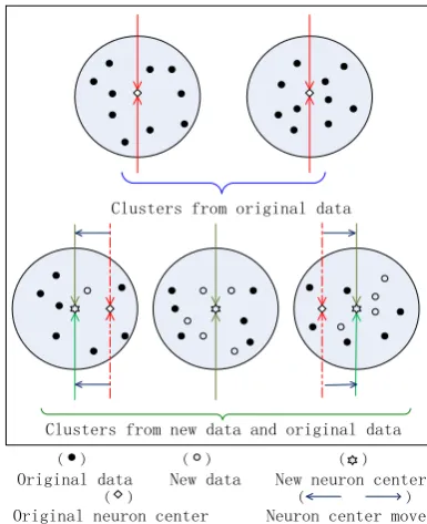
As indicated by [21,22], the best plan to perform incremental clustering is to combine the new added data and few samples chosen from the original data together to alter the clustering model that generates from the original data. If using this plan, the key is to detect the change of the distribution of the clusters when new data are added. This change is shown in Figure 3. In this figure, when new data are added, certain sparse area that is formed from the original data becomes dense and it will form a new cluster.
Neuron center move Clusters from new data and original data
Clusters from original data
Original data New data New neuron center
Original neuron center
( ) ( (
( (
) )
) )
Figure 3. The change of the distribution of the clusters after new data are added
3.1. Sample selection
In order to choose samples from the neuron model that is constructed from the original textual data, each cluster in our neuron model is separated into some compact sub-clusters. Then, samples are chosen from each sub-cluster to cover the information expressed by this sub-cluster. Local Density [23] is used to separate one cluster, since this algorithm frees of predefining neighborhood distance and neighborhood radius.
After each cluster is separated into some sub-clusters by Local Density, M samples are chosen to represent one sub-cluster. In the experiments (Figure 8), it can be found that when M reaches 3, clustering result is just acceptable. The reason is also shown after Figure 8.
( , ) - ( , ) ( , )
( , ) ( , )
j j
j
j j
Sim D BMN Sim D SMN R D BMN
Sim D BMN Sim D SMN
(7)
where BMN denotes the neuron that has the largest similarity to text Dj; it also represents the neuron that
Dj maps to; SMN denotes the neuron that has the
second similarity to Dj.
In Eq.(7), if the gap between Sim(Dj,BMN) and
Sim(Dj,SMN) is large, it means Dj is more similar to
the cluster that Dj maps to, and has less similarity to
the other clusters. It also means that Dj locates at the
center of the cluster that it belongs to. When the new texts appear, Dj may not move to another cluster. On
the contrary, if this gap is small, it means Dj locates at
the boundary of the cluster that Dj belongs to. When
the new texts appear, Dj may easily move to another
cluster. It also needs another text, whose relation is between the largest relation and the smallest relation, to represent the middle part of the sub-cluster. Thus, it can be concluded that when M reaches 3, the chosen samples can represent each location of the sub-cluster perfectly.
3.2. Incremental clustering
When the new texts appear, the samples chosen from the original texts can be combined with the new added texts together to train neuron model generated from the original texts. At the beginning of training process, because neuron model is only suitable for the original texts, the new added texts should take a more important status. This way can make neuron model simulate the distribution of the new texts rapidly. However, after running training process for a while, neuron model will be over trained and deviates from the distribution of the new texts. This is because only a few samples are chosen to represent the original texts. If the samples and the new texts have the same importance in training process, neuron model will be over trained and over simulate the new texts. For this reason, we use a threshold to separate training process into two parts, and different weights are evaluated on the samples along with training process. When the number of training steps is less than the threshold, neuron model is more suitable for the original texts. Then, samples are evaluated with lower weights to make neuron model simulate the new texts rapidly. When the number of training steps is larger than the threshold, that means training process runs for a while. At this moment, the weights of the samples are added to avoid “over training”. Based on this idea, Eq.(8) is formed to weigh the samples:
1;
( , 1) (2 ( )) ( , ) log( ( ));
j j j
If training steps W
W SD t a t R SD BMN SZ SD
If training steps W
(8)
where W denotes the threshold of the number of the steps to separate training process into two parts; SDj
denotes jth sample; Weight(SDj,t+1) denotes the
weight of SDj at t+1th training step; SZ(SDj) denotes
the size of the sub-cluster that SDj belongs to;
R(SDj,BMN) is calculated by Eq.(7).
The threshold W in Eq.(8) is empirically assigned the sum of the size of the new texts and the size of the samples. When the number of training steps is larger than W, the weight of the sample is adjusted. From the lower sub-equation in Eq.(8), it can be observed that the size of the sub-cluster and the relation between the sample and the neuron are used together to adjust the weight of the sample. On the one hand, if the size of the sub-cluster is larger, it means that the sample represents larger sub-cluster. Thus, the weight of the sample is higher. On the other hand, if the relation between the sample and the neuron is higher, it means that this sample can better represent the information expressed by the cluster that maps to this neuron. Thus, the weight of the sample is higher.
4. Experiments and analyses
In this paper, we construct a corpus including 107
news web pages downloaded from Yahoo website during the entire year of 2014 to test the performance of our algorithm. This corpus includes more than one thousand clusters, e.g. “society”, “military”, “sports”, “entertainment”, “policy”, “education”, “medicine”, “arts”, etc. Since this corpus is large-scale and downloaded from internet, it is impossible for users to manually partition it into several clusters and then apply certain measure, e.g. F1 or Purity, to measure clustering precision. Therefore, in this paper, ARI
(Adjusted Random Index) is adopted to measure clustering precision [24]. It evaluates how well the algorithm splits input data into different clusters by looking at the relation between the clusters, and not between the clusters and the given labels. With respect to ARI, it combines two texts as one pair-point. If the volume of text collection is n, this collection has n*(n -1)/2 possible pair-points.
ARI utilizes four situations to identify clustering result.
a) Two texts included by one pair-point are manually labeled in the same cluster, and in clustering result they are also in the same cluster.
b) Two texts included by one pair-point are manually labeled in the same cluster, and in clustering result they are in different clusters.
c) Two texts included by one pair-point are manually labeled in different clusters, and in clustering results they are also in different clusters.
d) Two texts included by one pair-point are manually labeled in different clusters, and in clustering result they are in the same cluster.
2
[ ]
2
[ ]
2
n
a c a b a d b c c d ARI
n
a b a d b c c d
(9)
Running time and clustering precision of VCLC with semantic initialization and random initialization are recorded in Figure 4 and Figure 5, respectively.
Figure 4. Running time of VCLC, respectively, with semantic initialization and random initialization
From Figure 4, it is easy to be found that running time of VCLC with semantic initialization is less than the one with random initialization. This is because semantic initialization makes the features that can better represent the topic of the cluster agglomerate together to form the initial neurons. This construction can form better initial cluster partition, which is close to the convergent partition. Thus, it only needs fewer iterative training steps to converge.
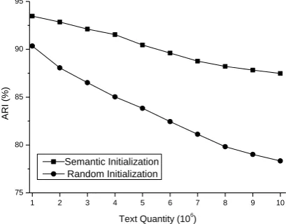
Figure 5. Clustering precision of VCLC, respectively, with semantic initialization and random initialization
From Figure 5, it can be found that VCLC with semantic initialization owns better clustering precision than the one with random initialization. The reason is that for most of clustering algorithms, initialization takes an important status to affect their precisions. Good initialization not only can accelerate clustering speed, but also can reduce the chance that texts map to
wrong clusters. Since semantic initialization partitions texts into the clusters that are separated well, the precision of VCLC with semantic initialization is better than the one with random initialization.
Together with iterative training process of SOM, our algorithm (VCLC) can further enhance its precision. Traditional SOM based algorithm applies vector based similarity measurement to calculate the similarity between neuron and text. This measurement is not fit to our algorithm, since we only choose a few features to represent one cluster. Therefore, a novel similarity measurement is proposed in this paper. In Table 1, we compare the measurement proposed in our paper (Eq.(4)) with the other popular measurements that are applied in SOM. The baseline measurements include Cosine, Euclidean distance, KL, SMTP [25], ADSS [26], and HLCL [27]. Because our algorithm (VCLC) compresses the feature set, the baseline similarity measurements cannot be directly applied in our algorithm for testing. To deal with this problem, we just apply the baseline measurements in SOM to run test.
Table 1. Clustering precision of different measurements
Measurements Cosine Euclidean KL
ARI (%) 75.46 76.03 76.18
ADSS SMTP HLCL VCLC
80.71 82.83 81.02 87.47
From Table 1, it is easy to be observed that different similarity measurements obtain the distinct clustering precisions. ADSS, SMTP, and HLCL obtain better precisions, since they all consider compressing vector. However, they never consider measuring the semantic similarity between the information that are, respectively, expressed by text and neuron. This fact causes that these three measurements obtain lower precisions than ours. For Cosine, Euclidean distance, and KL, these three similarity measurements are based on concurrence ratio and not only never consider compressing feature set but also never consider semantic similarity between text and neuron. Thereby, these three measurements obtain the lowest precisions. Compared with the six baseline measurements, our proposed measurement first uses initial step to keep the features that are semantically similar in one feature set, and then uses two situations to measure the similarity between neuron and text. Therefore, our proposed measurement obtains the highest precision.
In the initial step, the features that are semantically similar are chosen to compress feature set. After that, these compressed feature sets are fine-tuned through adjusting the similarity measurement and the neuron adjustment equation. That makes the initial step and the following training process integrate well, which means the initial step proposed in this paper can only be applied in our algorithm to obtain high precision. On the contrary, most of traditional algorithms run
1 2 3 4 5 6 7 8 9 10
300 400 500 600 700 800 900 1000 1100 1200
R
u
n
n
in
g
T
ime
(se
c)
Text Quantity (106
)
Semantic Initialization Random Initialization
1 2 3 4 5 6 7 8 9 10
75 80 85 90 95
AR
I
(%
)
clustering in uncompressed feature set. Though some of them compress feature set, they often separate clustering and initialization as two unrelated steps. Due to this isolation, it cannot ensure that the final clustering result can be improved by the initial step.
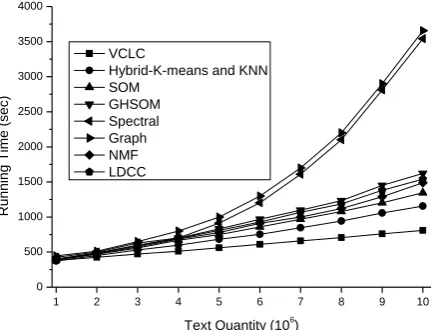
Running time and clustering precision of VCLC are also compared with some other well-known text clustering algorithms. They are Spectral Clustering [3], Graph Clustering [19], Hybrid of K-means and KNN [4], SOM [17], and an improved SOM based algorithm, GHSOM [18]. Two recently proposed clustering algorithms are also considered in the testing. They are Non-negative Matrix Factorization (NMF) [28], and LDCC based on Latent Dirichlet Allocation from Topic Model [29]. The results are shown in Figure 6 and Figure 7.
Figure 6. Running time of different algorithms
From Figure 6, it is easy to be found that running time of VCLC is the shortest. When text collection enlarges, the high time performance of VCLC is easier to be perceived. This is because VCLC has two advantages that can greatly reduce running time. One advantage is that VCLC chooses the features that can better represent the topic of the cluster to compress feature set. When the scale of text collection is small, for example smaller than 106, this compression has
little effect. At this time, running time of different algorithms is almost the same. Correspondingly, when the scale of text collection augments, compression begins to work. Running time of VCLC is obviously less than the other algorithms. When the scale of text collection reaches 3*106, VCLC can compress feature
set by 1/5000. It effectively reduces running time. The other advantage is that VCLC uses semantic similarity to construct the initial neuron model. Since this initial model is close to the convergent partition, it obviously decreases the number of iterative steps spent to reach convergence. From Figure 6, it can also be found that the rank of running time spent by the other baseline algorithms from low to high is Hybrid of K-means and KNN, SOM, NMF, LDCC, GHSOM, Spectral Clustering, and Graph Clustering. Time complexities of Hybrid of K-means and KNN, SOM, and GHSOM are all O(kln) [5,17,18], where k is cluster quantity; l
is the number of iterative steps; n is text quantity. The rank of the numbers of iterative steps spent by these three algorithms from low to high is Hybrid of K-means and KNN, SOM, and GHSOM. Therefore, the rank of running time spent by them from low to high is KNN, SOM, and GHSOM. The other two algorithms, Spectral Clustering and Graph Clustering, need to decompose matrix. Thus, they spend the longest running time. For NMF, it applies matrix decomposition to reduce the dimension of feature space. In this low-dimensional feature space, NMF runs much faster and also obtains more precise result. However, if we consider the matrix decomposition process as the preprocessing step of clustering process, its running time is high and even more than SOM. The reason is that time complexity of decomposition is beyond linear against the size of text collection. Therefore, NMF spends much more time when text collection enlarges. For LDCC, space transformation is used. LDCC transforms feature space to topic model, and extracts topics from text collection to separate texts into several clusters of different topics. This way can enhance clustering precision, whereas due to the added transformation step, its running time is also longer. In fact, as show in [1], among most of recent clustering algorithms proposed to enhance clustering precision, the linear time complexity (like SOM and K-means) can be treated as the ideal time complexity.
Figure 7. Clustering precision of different algorithms
From Figure 7, it is easy to be found that the rank of clustering precision from low to high is Hybrid of K-means and KNN, SOM, GHSOM, Spectral Clustering, Graph Clustering, NMF, LDCC, and VCLC. There are two reasons to the situation that VCLC has the highest precision. First of all, VCLC uses semantic similarity to construct an initial neuron model. This model reduces the interferences brought from the wrongly partitioned texts. Secondly, VCLC chooses the features that are related to the topic of the cluster to construct the feature set of one cluster and filters the interferences brought from the unrelated features. This method can greatly increase the
intra-1 2 3 4 5 6 7 8 9 10
0 500 1000 1500 2000 2500 3000 3500 4000
R
u
n
n
in
g
T
ime
(se
c)
Text Quantity (106 ) VCLC
Hybrid-K-means and KNN SOM
GHSOM Spectral Graph NMF LDCC
1 2 3 4 5 6 7 8 9 10
65 70 75 80 85 90 95
AR
I(%
)
Text Quantity (106 ) VCLC
Hybrid-K-means and KNN SOM
cluster agglomeration and the inter-cluster distinctness. Precisions of Spectral Clustering, Graph Clustering, SOM, and GHSOM are lower than VCLC. These four algorithms all map a high dimensional data space into a low dimensional transition space to cluster texts. Thus, their precisions are similar. However, since all of them never consider removing the features that are unrelated to the topic of the cluster, their precisions are lower than VCLC. Clustering precision of Hybrid of K-means and KNN drops rapidly, when the scale of text collection augments. That means this algorithm is only suitable for clustering small-scale text collection. The reason to this situation is that Hybrid of K-means and KNN applies Vector Space Model to organize texts and clusters. This model cannot solve the problem of “curse of dimensionality”. For NMF and LDCC, they either use matrix decomposition (NMF) or topic model (LDCC) to enhance their precisions. More importantly, when text collection is large, these two algorithms do not lose their precisions either. The reason is that matrix decomposition and topic model applied by NMF and LDCC not only can reduce the dimension of feature space but also can extract the key features from text to enhance clustering precision. Therefore, NMF and LDCC obtain the similar precision to our algorithm (VCLC). However, since VCLC considers the similar features in the adjustment equation, it can aggregate the semantically similar texts into one cluster. Compared with VCLC, NMF and LDCC cannot cluster semantically similar texts. Therefore, VCLC obtains higher precision than NMF and LDCC.
In the following experiments, the performance of the incremental version of VCLC (i.e. I-VCLC) is tested. Figure 8 shows the precision of I-VCLC, when it combines the new added texts and the samples of different numbers chosen from the original texts to perform incremental clustering.
Figure 8. Clustering precision of I-VCLC when different numbers of samples are chosen
From Figure 8, it is easy to be found that when the numbers of the samples chosen from the original texts are different, I-VCLC obtains the distinct precisions.
When this number is less than 3, precision drops rapidly. This is because when this number equates to 1, only the text that can represent the center of the sub-cluster or the boundary of the sub-cluster is sampled. When this number equates to 2, two texts that can represent the center of the sub-cluster and the boundary of the sub-cluster are sampled, whereas it neglects to sample the text that can represent the middle part of the sub-cluster. When this number equates to 3 or is much higher, the chosen samples can represent one sub-cluster well. Thus, the precision curve becomes smooth.
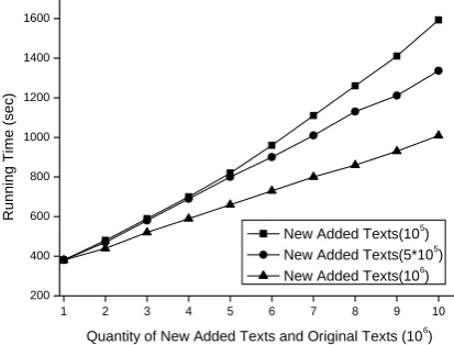
To simulate incremental clustering, 106 texts that
are randomly chosen from testing corpus are used as the original texts to form an initial neuron model using VCLC. After that, we randomly select different scales of texts each time, e.g. 105, 5*105, and 106, to perform
incremental clustering using I-VCLC. These selected texts are treated as the new added texts, and they are combined with the samples chosen from the original texts to perform incremental clustering using I-VCLC. Each time when the sum of the quantity of the original texts and the quantity of the new added texts equates to the integral times of 106, clustering precision and
running time are, respectively, recorded once in Figure 9 and Figure 10.
1 2 3 4 5 6 7 8 9 10
200 400 600 800 1000 1200 1400 1600
R
u
n
n
in
g
T
ime
(se
c)
Quantity of New Added Texts and Original Texts (106) New Added Texts(105) New Added Texts(5*105
) New Added Texts(106
)
Figure 9.Running time of I-VCLC when the new texts of different scales are added
From Figure 9, it is easy to be found that when the sum of the quantity of the original texts and the quantity of the new added texts is small, running time of I-VCLC is similar though the new added texts are of different scales. The reason is that when this sum is small, each sub-cluster only includes few texts. At this moment, the samples chosen from one sub-cluster are almost all the texts in this sub-cluster. In this situation, running time of I-VCLC is very similar no matter whichever quantity of the new texts is added. By contrast, when this sum enlarges, running time of I-VCLC is different in the situation that the new added texts are of different scales. There are two reasons to this situation. First of all, if more texts are inserted as the new texts at each incremental time, it only needs fewer times to perform incremental clustering when the sum of the quantity of the original texts and the
1 2 3 4 5 6 7 8 9 10
65 70 75 80 85 90
AR
I
(%
)
quantity of the new texts reaches certain scale. For example, if we select texts in the scale of 105 each
time to perform incremental clustering, when this sum reaches 2*106, it has to perform incremental clustering
ten times (the quantity of the original texts is 106); if
we select 5*105, it needs two times; if we select 106, it
only needs one time. Secondly, the new added texts are sampled from testing corpus. Then, if more texts are inserted at each incremental time, neuron model will be more similar to the distribution of testing corpus. In this situation, it only needs to choose fewer samples to represent one sub-cluster. Thus, the quantity of the texts that need to be incrementally clustered is smaller, which causes less running time.
1 2 3 4 5 6 7 8 9 10
70 75 80 85 90 95
AR
I
(%
)
Quantity of New Added Texts and Original Texts (106) New Added Texts(105)
New Added Texts(5*105 ) New Added Texts(106)
Figure 10. Clustering precisionof I-VCLC when the new texts of different scales are added
From Figure 10, it is easy to be found that there are two trends along with x-axis and y-axis. Along with x-axis, clustering precisions all drop no matter whichever scale of the new texts is used. Since the new added texts are randomly selected from testing corpus, the distribution of the new added texts is only approximate to the distribution of testing corpus. However, after performing incremental clustering for several times, the distribution of neuron model (or cluster model) may deviate from the distribution of testing corpus. Then, when the new texts are added, they will distort the distribution of neuron model. Therefore, clustering precision drops along with the augment of the quantity of the total texts. Along with y-axis, clustering precision is much higher if more new texts are added at each incremental time. This is because when more new texts are added at each incremental time, the distribution of the new added texts is more approximate to the distribution of testing corpus. Then, it affects the distribution of neuron model a little. Therefore, clustering precision is higher, if more new texts are added at each incremental time.
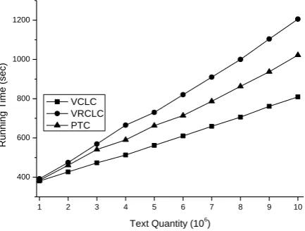
In Figure 11 and Figure 12, we compare the algorithm proposed in this paper (VCLC) with the algorithms (VRCLC and PTC) proposed in our early
papers [8,20] on clustering precision and running time.
Form Figure 11, it can be found that our algorithm (VCLC) owns the highest time performance. Its running time is less than that of VRCLC and PTC. Besides, when the scale of text collection enlarges, its running time shortens much compared with VRCLC and PTC. There are two reasons to this situation. One is that our algorithm first partitions texts into several initial clusters via semantic similarity. This initial cluster partition is close to the final cluster partition, which can be seen from Figure 5. Therefore, our algorithm (VCLC) spends less running time than VRCLC and PTC. The other reason is that in the neuron adjustment step, VCLC considers the features that are similar to the adjusted feature. This type of adjustment expands the range of the adjustment on features. Therefore, it decreases running time. When the scale of text collection enlarges, more similar features exist in the feature space. Therefore, running time decreases much when the size of text collection enlarges. Compared with VCLC, VRCLC proposed in [8] does not utilize any method to accelerate running speed. PTC in [20] tries to set a limitation on the size of feature set to accelerate running speed. Therefore, running time spent by PTC is less than that spent by VRCLC. However, since PTC does not try to apply initialization to save running time and also does not consider expanding the range of the adjustment on features, its running time is longer than VCLC.
Figure 11.Running time of VCLC, VRCLC, and PTC
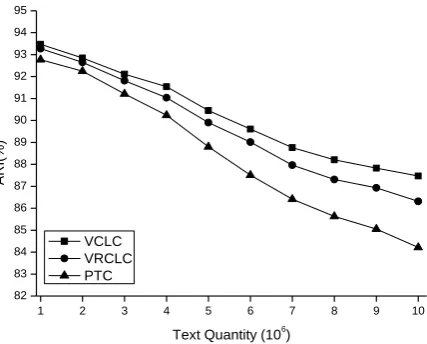
Form Figure 12, it can be found that our algorithm (VCLC) performs a little better than VRCLC and PTC when the size of text collection is small, and when this size enlarges to a certain level (e.g. more than 3*106),
the superiority of the precision of VCLC is easy to be perceived. The reason to this phenomenon is that our algorithm (VCLC) considers the similar features in its adjustment step, this type of adjustment can make the texts owning the similar features but not the same features (e.g. one text uses “computer” as its feature and one text uses “calculating machine” as its feature; these two texts are semantically similar) aggregate into one cluster. When the size of text collection
1 2 3 4 5 6 7 8 9 10
400 600 800 1000 1200
R
u
n
n
in
g
T
ime
(se
c)
Text Quantity (106) VCLC
enlarges, more texts are semantically similar. In this situation, our algorithm (VCLC) can find more semantically similar texts to enhance its precision. On the contrary, for VRCLC, it has two steps. One step runs iterative tuning process of SOM to adjust the features in the cluster vector. The second step reconstructs cluster vector by choosing the features related to the topic of the cluster to enhance precision. Unfortunately, these two steps run for two distinct objectives. The adjustment step aims at partitioning texts into separated clusters and the feature selecting step tries to find more similar features to represent cluster. The discrepancy in the purposes of these two steps often makes the clustering result obtained by VRCLC deviate from the precise result. Therefore, the precision obtained by VCLC is higher than that obtained by VRCLC. For PTC, it sets a threshold to limit the size of feature set and employs feature’s weight as criteria to choose features. Due to the fact that some important features may have little weights and thereby are removed from feature set, PTC owns the lowest precision among the three algorithms.
Figure 12. Clustering precision of VCLC, VRCLC, and PTC
5. Conclusion
A novel clustering algorithm for large-scale text collection (abbreviated as VCLC) is proposed in this paper. This algorithm selects the features that are related to the topic of the cluster to construct feature set as the representation of this cluster. This method not only can increase intra-cluster agglomeration and inter-cluster distinctness, but also can compress feature set by 1/5000 to extremely reduce running time. Besides, iterative training process of self-organizing-mapping (SOM) is imported to fine-tune the weights of the selected features. Based on this idea, one feature set is treated as one neuron, and a novel similarity measurement and a novel neuron adjustment equation are also proposed. To further reduce running time and finally to obtain the precise clustering result, semantic similarity is used to initialize a neuron model. Furthermore, since new
texts appear in website every day, this paper also proposes an incremental version of VCLC (abbreviated as I-VCLC) to cluster unstable texts. Experimental results demonstrate that VCLC can cluster large-scale text collection at high precision, and I-VCLC can cluster texts at any time when new texts appear.
Acknowledgments
The research in this paper is supported by National Natural Science Foundation of China (No.61300114), Specialized Research Fund for the Doctoral Program of Higher Education (No.20132302120047), the Special Financial Grant from the China Postdoctoral Science Foundation (No.2014T70340), China Postdoctoral Science Foundation (No.2013M530156), the Fundamental Research Funds for the Central Universities (No.HIT.NSRIF.2013066), CCF-Tencent Open Fund (No.CCF-TencentIAGR 20140109), 2015 Guangdong Provincial Key Platform Project-the Youth Innovative Talent Funding.
References
[1] R. Xu, D. Wunsch. Survey of clustering algorithms. IEEE Transactions on Neural Networks, 2005, Vol. 16, No. 3, 645-678.
[2] R. Agrawal, J. Gehrke, D. Gunopulos, P. Raghavan.
Automatic subspace clustering of high dimensional data for data mining applications. In: Proceedings of the 1998 ACM SIGMOD International Conference on Management of Data, 1998, pp. 94-105.
[3] L. Jing, M. K. Ng, T. Zeng. Dictionary learning-based subspace structure identification in spectral clustering. IEEE Transactions on Neural Networks and Learning Systems, 2013, Vol. 24, No. 8, 1188-1199.
[4] C. Dhanjal, R. Gaudel, S. Clémençon. Efficient eigen-updating for spectral graph clustering. Neurocomputing, 2014, Vol. 131, 440-452.
[5] H. Ramin, K. Kamal. A new hybrid means and k-nearest-neighbor algorithms for text document clustering. International Journal of Academic Research, 2014, Vol. 6, No. 3, 79-84.
[6] Z. Liu, K.-C. Chiu, L. Xu. Improved system for object detection and star/galaxy classification via local subspace analysis. Neural Networks, 2003, Vol. 16, No. 3, 437-451.
[7] W. Song, S. C. Park. Genetic algorithm for text clustering based on latent semantic indexing. Computers & Mathematics with Applications, 2009, Vol. 57, No. 11, 1901-1907.
[8] M. Liu, C. Wu, L. Chen. A vector reconstruction based clustering algorithm particularly for large-scale text collection. Neural Networks, 2015, Vol. 63, 141-155.
[9] C. C. Aggarwal. On change diagnosis in evolving data stream. IEEE Transactions on Knowledge and Data Engineering, 2005, Vol. 17, No. 5, 587-600.
[10] M. Spiliopoulou, I. Ntoutsi, Y. Theodoridis, R. Schult. MONIC-modeling and monitoring cluster transitions. In: Proceedings of the 12th ACM SIGKDD
1 2 3 4 5 6 7 8 9 10
82 83 84 85 86 87 88 89 90 91 92 93 94 95
AR
I(%
)
Text Quantity (106) VCLC
International Conference on Knowledge Discovery and Data Mining, 2006, pp. 706-711.
[11] R. G. Pensa, D. Ienco, R. Meo. Hierarchical co-clustering: off-line and incremental approaches. Data Mining and Knowledge Discovery, 2014, Vol. 28, 31-64.
[12] R. Lang, K. Warwick. The plastic self organising map. In: Proceedings of the 2002 International Joint Conference on Neural Networks, 2002, pp. 727-732. [13] T. Kohonen. Self-organizing maps. Springer, Berlin,
1997.
[14] M. Galley, K. Mckeown. Improving word sense disambiguation in lexical chaining. In: Proceedings of the Eighteenth International Joint Conference on Artificial Intelligence, 2003, pp. 1486-1488.
[15] H. Peng, F. Long, C. Ding. Feature selection based on mutual information: Criteria of dependency, max-relevance, and min-redundancy. IEEE Transactions on Pattern Analysis and Machine Intelligence, 2005, Vol. 27, No. 8, 1226-1238.
[16] K. Tasdemir, P. Milenov, B. Tapsall. Topology-based hierarchical clustering of self-organizing maps. IEEE Transactions on Neural Networks, 2011, Vol. 22, No. 3, 474-485.
[17] D. Alahakoon, S. K. Halgamuge, B. Srinivasan.
Dynamic self-organizing maps with controlled growth for knowledge discovery. IEEE Transactions on Neural Networks, 2000, Vol. 11, No. 3, 601-614. [18] A. Rauber, D. Merkl, M. Dittenbach. The growing
hierarchical self-organizing map: Exploratory analysis of high-dimensional data. IEEE Transactions on Neural Networks, 2002, Vol. 13, No. 6, 1331-1341. [19] A. Aizawa. An information-theoretic perspective of
tf-idf measures. Information Processing and Manage-ment, 2003, Vol. 39, No. 1, 45-65.
[20] M. Liu, Y. Liu, B. Liu, L. Lin. Probability-based text clustering algorithm by alternately repeating two operations. Journal of Information Science, 2013, Vol. 39, No. 3, 372-383.
[21] E. Lughofer. Extensions of vector quantization for incremental clustering. Pattern Recognition, 2008, Vol. 41, No. 3, 995-1011.
[22] H. Liu, X. Ban. Clustering by growing incremental self-organizing neural network. Expert Systems with Applications, 2015, Vol. 42, Issue 11, 4965-4981. [23] L. Duan, L. Xu, F. Guo, J. Lee, B. Yan. A
local-density based spatial clustering algorithm with noise. Information Systems, 2007, Vol. 32, No. 7, 978-986. [24] Y. Zhao, G. Karypis. Criterion functions for
document clustering: Experiments and analysis. Technical Report, #01-40, University of Minnesota, 2002.
[25] G. Pirró. A semantic similarity metric combining features and intrinsic information content. Data and Knowledge Engineering, 2009, Vol. 68, Issue 11, 1289-1308.
[26] L. Han, L. Sun, G. Chen, L. Xie. ADSS: An approach to determining semantic similarity. Advances in Engineering Software, 2006, Vol. 37, No. 2, 129-132.
[27] M. Yazdani, A. Popescu-Belis. Computing text semantic relatedness using the contents and links of a hypertext encyclopedia. Artificial Intelligence, 2013, Vol. 194, 176-202.
[28] N. Del Buono, G. Pio. Non-negative Matrix Tri-Factorization for co-clustering: An analysis of the block matrix. Information Sciences, 2015, Vol. 301, Issue C, 13-26.
[29] A. Gross, D. Murthy. Modeling virtual organizations with Latent Dirichlet Allocation: A case for natural language processing. Neural Networks, 2014, Vol. 58, 38-49.