Using a generalized additive model with autoregressive terms to study the effects of daily temperature on mortality

R E S E A R C H A R T I C L E

Open Access

Using a generalized additive model with

autoregressive terms to study the effects of daily

temperature on mortality

Lei Yang

, Guoyou Qin

, Naiqing Zhao

, Chunfang Wang

and Guixiang Song

Abstract

Background:Generalized Additive Model (GAM) provides a flexible and effective technique for modelling nonlinear time-series in studies of the health effects of environmental factors. However, GAM assumes that errors are mutually independent, while time series can be correlated in adjacent time points. Here, a GAM with Autoregressive terms (GAMAR) is introduced to fill this gap.

Methods:Parameters in GAMAR are estimated by maximum partial likelihood using modified Newton’s method, and the difference between GAM and GAMAR is demonstrated using two simulation studies and a real data example. GAMM is also compared to GAMAR in simulation study 1.

Results:In the simulation studies, the bias of the mean estimates from GAM and GAMAR are similar but GAMAR has better coverage and smaller relative error. While the results from GAMM are similar to GAMAR, the estimation procedure of GAMM is much slower than GAMAR. In the case study, the Pearson residuals from the GAM are correlated, while those from GAMAR are quite close to white noise. In addition, the estimates of the temperature effects are different between GAM and GAMAR.

Conclusions:GAMAR incorporates both explanatory variables and AR terms so it can quantify the nonlinear impact of environmental factors on health outcome as well as the serial correlation between the observations. It can be a useful tool in environmental epidemiological studies.

Background

People have long been interested in potential impacts of temperature on human health [1-3]. Recently, many studies have been done to analyse the way and the ex-tent temperature influences health outcomes [4-6]. Such studies have practical value for the following reasons: knowing the association between environmental factors and health outcomes will help to identify at-risk popula-tions, benefit health department in resource allocation, and provide support for stake holders in prevention [7].

Environmental epidemiology, the investigation of the health risks related to environmental exposures, becomes the main research approach [8]. There are vari-ous study designs in environmental epidemiology for es-timating health effects of temperature. One of them is

model evaluation of time series data to quantify the association between temperature (or other weather/ environmental factors etc.) and daily mortality (or hospitalization etc.). These are a type of ecologic study because they analyse daily population-averaged health outcomes and exposure levels [9]. This approach is suit-able to study transient acute effects which are due to time-varying exposures [10-14], and the choice of model can have a large influence on the interpretation of envir-onmental effects.

Generalized Linear Model (GLM) [15] and General-ized Additive Model (GAM) [16] are the main models used in environmental epidemiology. When the response variable represents counts (e.g. number of deaths), the model often takes the form of a Poisson regression/addi-tive model with a log link function. The outcome Ytis assumed to follow a Poisson distribution with mean μt which is linked either to a linear combination (in this case, the model is a GLM) or smoothed functions (in

* Correspondence:[email protected]

1

Department of Biostatistics, School of Public Health, Fudan University, Shanghai, China

Full list of author information is available at the end of the article

this case, the model is a GAM) of environmental ex-planatory variables via a log function.

Many studies have identified the nonlinear relations (U, J, or V shaped) of daily mortality on temperature [17-24], which are mainly represented by piecewise lin-ear terms [18-20] or natural cubic splines [21-24]. An assumption is often made that temperature only affects the mortality of the same day or on a single day of lag l [18,20-22], and denoted by the term tempt-l in the model. When l=0, it represents the effect on the same day [18,20-23], when l>0, it represents a lagged effect [18,20,21,23]. An alternative to single lag models is a dis-tributed lag model [25]. It includes multiple lags of temperature over a period of time based on the assump-tion that the effect of time is distributed over several days into the future. In all the above models, a spline function of time is often used to explain the long time trend, and confounding effects like humidity and air pol-lution are also controlled by splines.

However, a thorough time series analysis should con-sider the order of data points and correlation of adjacent points in time [26]. In environmental epidemiological studies, the response variable may also be correlated and it is necessary to embody autocorrelation of the response variable when modelling. But all the above models are standard GLM/GAM that describes how the response variable is stochastically related to explanatory variables without considering how the response can be dependent also on its past values.

In addition, autocorrelation causes trouble in

estima-tion of GLM/GAM, since GLM/GAM essentially

requires each observation to be independently distribu-ted. Violation of this assumption can lead to problematic estimates even in very simple cases. For example, if the error terms in a linear regression model are in reality positively autocorrelated, failure to account for this may underestimate the standard errors of the estimated re-gression coefficients [27].

Another statistical issue often encountered is overdis-persion, and many sources of autocorrelation are related to sources of overdispersion [28]. One usual approach to adjust for overdispersion is to specify a dispersion par-ameterφfor estimation [15]. However, if autocorrelation exists, this approach only inflates the variance of the es-timate byφbut leaves the estimate unchanged, which is an inadequate solution to our issue.

Generalized Estimating Equations (GEE) [29,30] and Generalized Linear Mixed Model (GLMM)/Generalized Additive Mixed Model (GAMM) [31,32], are two exten-sions from GLM/GAM for grouped or clustered data. GEE and GLMM/GAMM can be implemented in popu-lar software like SAS and R [31-34]. For all these models, a within-group variance-covariance structure can be used to account for the corresponding within-group

autocorrelation [31,34]. Time series data, treated as sin-gle cluster data, can also be modelled by GAMM. Per-formance of this degenerative GAMM will be studied in simulation.

In this article, we introduced GAM with Autoregres-sive terms (GAMAR), which is derived from Generalized Autoregressive Moving Average (GARMA) models [35]. ARMA is a family of models for analysing time series. The notation ARMA(p,q) refers to a model with p auto-regressive terms and q moving-average terms [26]. GARMA belongs to the class observation driven models [36] for extending Gaussian ARMA to non-Gaussian set-tings. GAMAR differs from GARMA in that the linear components in GARMA are generalized to natural splines and MA terms are omitted. The generalization is motivated by modelling nonlinear relationships, while the simplifica-tion is justified because AR can be used to approximate MA or ARMA. Additionally, larger AR order in GAMAR will not compromise the estimation of the effects of ex-planatory variables.

In all, GAMAR has two advantages over GAM: 1) it is a model for generalized time series analysis rather than a probabilistic model like GAM; 2) the AR part of GAMAR can explain the autocorrelation structure of observations. So the Pearson residuals of GAMAR can be closer to white noise than those from GAM, yielding more reliable estimation.

Methods GARMA

In GARMA, the conditional distribution of each obser-vation yt, for t=1,. . .,n, given the previous information set Ht={X1,. . .,Xt,y1,. . .,yt-1} containing past observations

ytand covariate vectors Xt= (Xt1,. . .,Xtm), is assumed to follow the same exponential family distribution [35]. As with the standard GLM, the conditional mean μt is related to the variables by a twice-differentiable one-to-one monotonic function g, which is called the link function. However, unlike the standard GLM, the for-mula here allows autoregressive moving average terms to be included additively [35]:

gð Þ ¼μ_t X

m

i¼1 Xtiβiþ

Xp

j¼1

cj g ytj

Xm

i¼1 Xtj;iβi

!

þX

q

j¼1

dj g ytj

g μ_tj

;

where X

p

j¼1

cj g ytj

Xm

i¼1 Xtj;iβi

!

are autoregressive

terms and X

q

j¼1

dj g ytj

g μ_tj

are moving

Count data are often assumed to follow Poisson distri-bution. And the Poisson GARMA submodel is:

lnðE yð Þt Þ ¼lnð Þ ¼μt Xm

i¼1 Xtiβi

þX

p

j¼1

cj ln ytj

Xm

i¼1 Xtj;iβi

!

þX

q

j¼1

dj ln ytj=μtj

;

whereyt*= max(yt,τ),τis a positive threshold parameter. Any 0 or negative values of y are replaced byτ, because ln() is not defined for 0 or negative values.

GAMAR

GAMAR is derived from GARMA with linear terms replaced by smoothers and MA terms omitted:

g E yð ð Þt Þ ¼gð Þ ¼μt Xm

i¼1 sið ÞXti

þX

p

j¼1

cj g ytj

Xm

i¼1 si Xtj;i

!

; ð1Þ

where X

m

i¼1

sið ÞXti are smoothers of covariates, Xp

j¼1

cj g ytj

Xm

i¼1

siXtj;i !

are autoregressive terms.

Compared to GAM, (1) allows autoregressive terms to be included additively in the link predictor.

For count data y, we use the Poisson submodel:

lnðE yð Þt Þ ¼lnð Þ ¼μt Xm

i¼1 sið ÞXti

þX

p

j¼1

cj ln ytj

Xm

i¼1 si Xtj;i

!

; ð2Þ

hereyt*= max(yt,τ),τis a positive threshold parameter. In our study, we use natural cubic spline (ns) as smoother. ns is a piecewise-cubic real function on an interval [a,b], where [a,b] is separated by a sequence of k ordered knots: α = ξ0 < ξ1 < ⋯ < ξk-1 < ξk = b.

ns is continuous at interior knots and linear beyond the boundary [16]. Degrees of freedom (df) for ns

equals to the number of subintervals separated by these knots, thus df satisfies: df = k. ns is often represented by linear combination of its B-spline basis [16]. When df is specified, the standard practice is to place df-1 interior knots at evenly spaced inter-vals in the data to generate the B-spline basis. By using ns as smoother in (2), the Poisson GAMAR

becomes:

lnðE yð Þt Þ ¼lnð Þ ¼μt Xm

i¼1

ns Xð it;dfiÞ

þX

p

j¼1

cj ln ytj

X

m

i¼1

ns Xij;t;dfi

!

:

Algorithm

Maximum partial likelihood estimator (MPLE)

For the jointly distributed time series {Xt,yt}, t = 1,. . .n, the parameters of GAMAR can be estimated by max-imum partial likelihood. The partial likelihood based on

ytfor {Xt,yt}, t = 1,. . .ncan be expressed as the product of a sequence of conditional likelihoodsf(yt| X(t),y(t-1);θ),

t = 1,. . .n, whereX(t)= X1,. . .Xt,y(t-1)=y1,. . .yt-1, that is:

PL¼Y

n

t¼1

f ytXð Þt ;yðt1Þ;θ

:

This function is referred to as a partial likelihood in-stead of likelihood because Xt are stochastic [35]. For a Poisson GAMAR, the partial likelihood is:

PL¼Y

n

t¼1

μyt t

yt!

eμt;

and μt can be expanded as lnð Þ ¼μt Xm

i¼1

ns Xð ti;dfiÞ þ Xp

j¼1

cj ln ytj

Xm

i¼1

ns Xtj;i;dfi

!

. Since a natural

cubic spline is a linear combination of its B-spline basis, it is linear with respect to its parameters, so natural cubic spline functions are like linear terms from the per-spective of computation. Therefore,

lnð Þ ¼μ_t η_t ¼X m

i¼1

βiXti

þX

p

j¼1

cj ln ytj

Xm

i¼1

βiXtj;i !

ð3Þ

where θ = (β1⋯,βm,c1,⋯,cp)T is the model parameter vector.

Modified Newton’s method

Maximum partial likelihood estimators are solved by modified Newton’s method. This procedure is described in detail in Appendix.

Evaluation of GAMAR by simulation

for estimation. In simulation study 1, the performance of GAMM is also studied. The R code for simulations and simulation output is included in Additional file 1.

Simulation study 1

The first model:

Yt∼PoissonðμtÞ lnðμ_tÞ ¼nsðxt;5Þ þat

nsðxt;5Þ ¼ X5

i¼1

βisi5ð Þxt

at¼ X3

i¼1

ciðlnðy∗tiÞ ns xð ti;5ÞÞ

y_t ¼ maxðy;τÞ;τ¼0:5:

ð4Þ

Here xtrepresents a daily averaged temperature series from year 2000–2008 obtained from Shanghai's Me-teorological Bureau, and the termssi5(xt),i= 1, 2, 3, 4, 5 form the B-spline basis for the natural cubic spline. The parameters are:

β0¼5:02;β1¼ 0:35;β2¼ 0:36;β3¼ 0:38;β4

¼ 0:33;β₅¼ 0:15 and c1¼0:5;c2¼0:25;c3

¼0:12:

We used data ranging over time points 1828–3288 (year 2005–2008) to eliminate the impact of the starting value, where the time points stand for the days since Jan 1st 2000.

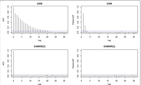
For two models on Sample 1, the Autocorrelation Function (ACF) and Partial Autocorrelation Function (PACF) [26] of the Pearson residuals [15] are plotted against different lag periods to examine the presence of residual autocorrelation. Estimates of temperature effects from the two models and the true effect were plotted against temperature to show which model provided a better fit.

Besides showing the analysis for a single sample, the averaged results from GAM, GAMM and GAMAR were given, and the statistics calculated were mean estimates, bias, relative error and coverage, short for

“coverage rate of confidence interval (CI) on true value”. The confidence level was chosen to be 95%, so the coverage of a correct model should be around 95%.

In addition, GAMAR with various AR orders were studied to explore the effects of AR order on estimation. Finally, to verify the consistency of partial maximum likelihood estimation, 1000 samples in the time range of 2558–3288 (2 years), 1828–3288 (4 years), 1097–3288 (6 years) were used for calculation.

Simulation study 2

A second simulation study was performed to study whether the proposed method could approximate a non-linear curve. We simulated 1000 samples from a model where the covariate is a cosine function of temperature and nonlinear with respect to the parameters.

Yt∼PoissonðμtÞ

lnðμ_tÞ ¼4:8þ0:2 cosðπðxtþ3Þ=28Þ þat

at¼ X3

i¼1

ci ln yti

ð4:8þ0:2 cosðπðxtþ3Þ=28ÞÞ

y_t ¼ maxðy;τÞ;τ¼0:5

ð5Þ Here, the AR terms parameters are identical to (4):c1= 0.5,c2= 0.25,c3= 0.12.

As in simulation study 1, sample statistics were cal-culated over the time points 1828–3288 (year 2005– 2008) for each of the 1000 realizations by GAM and GAMAR. The first sample was analysed just the same way as in simulation study 1, but here the mean and standard deviation of the parameter estimates from the two models for the 1000 samples are presented. To compensate for the absence of true parameters, we compared the two models visually, plotting the mean predicted values from the two models and the true ef-fect. Moreover, the Pearson correlation coefficients of the fitted linear predictors from the two models and true effect were also calculated.

Application to temperature-mortality research

The real example came from three sources: daily mortal-ity of Shanghai in 2001–2004 from Shanghai Municipal Center for Disease Control & Prevention; daily average temperature and humidity in 2001–2004 from Shanghai's Meteorological Bureau; and air pollution data (NO2, SO2, PM10) in 2001–2004 from (http://www.envir.gov. cn/airnews/), which was announced by the Shanghai En-vironmental Monitoring Centre.

Autocorrelation of the Pearson residuals from the two models are compared via figure. We also com-pared their parameter estimates, and their estimated temperature effects via figures. The R code for real example modelling and its outputs is included in Additional file 1.

Results

Simulation results Simulation study 1

3, it is natural to use GAMAR(3) instead. The model is given below:

lnðEðytÞÞ ¼nsðxt;5Þ þ X3

i¼1

ciðlnðy∗tiÞ ns xð ti;5ÞÞ

y_t ¼ maxðy;τÞ;τ¼0:5

ð6Þ

The ACF and PACF plot of the GAMAR(3) Pearson residuals suggest no autocorrelation, and the dispersion parameter estimate is now φ^ ¼1:0219≈1, indicating no overdispersion. Apparently, GAMAR(3) controls autocorrelation and overdispersion simultaneously, and Figure 2 indicates that the predicted spline

function = =

nsðx;5Þ from GAMAR(3) is much closer to the real model than that from GAM.

Concerning the general performance of GAM and GAMAR, Table 1 shows that the biases of the mean par-ameter estimates from GAM are almost the same as GAMAR. However, the coverages of the 95% confidence intervals from GAM are far less than 95%, while those from GAMAR are very close to 95%. Also, relative errors

of the parameter estimates from GAM are larger than that of GAMAR.

Coverages for GAM corrected for overdispersion [15] are also shown in Table 1 as coverage2. This approach is the same as a standard GAM except that its standard error has been expanded by the dispersion parameterφ. As a result, the bias and relative errors remain unchanged, while the Figure 1ACF and PACF of GAM and GAMAR(3) for Sample 1 from simulation study 1.These statistics are calculated on Pearson residuals

zt¼^ytffiffiffiyt ^ yt

p from both models.

confidence interval is broadened, coverage improved. How-ever, the coverage is still far less than 95%.

The results of GAMM with AR(3) correlation struc-ture and GAMAR(3) are very similar, but the former model is much more time consuming. This disparity will be described in discussion. Hence results from only 50 samples fitted by GAMM are summarized in Table 1.

To examine how the AR order in GAMAR influences the results, we also fitted the GAMAR(1), GAMAR(2), GAMAR(4), and GAMAR(5). As Table 1 in Additional file 2 shows, the coverage grows and relative error drops as the AR order increases from 1 to 3. For models with AR order larger than 3, there is little difference in cover-age, relative error and bias among them.

The results for different time ranges are listed in Table 2 in Additional file 2, from which we can see that the larger the number of time-points, the lower the bias and relative errors, and the higher the coverage. This illustrates the asymptotic unbiased (consistency) prop-erty of MPLE.

Simulation study 2

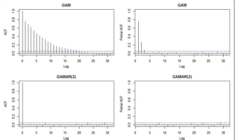
In this simulation study, The ACF and PACF plot of the GAM Pearson residuals from the first sample also reveal obvious autocorrelation (Figure 3). Just as in simulation study 1, we can see that ACF tails off and PACF cuts off after lag 3 for GAM, suggesting AR(3) would be suitable. In contrast, the ACF and PACF of GAMAR(3) on the same data are both very close to 0. And Figure 4 indi-cates that the predicted spline function nsðx= =;5Þ from

GAMAR(3) is much closer to the real model than that from GAM.

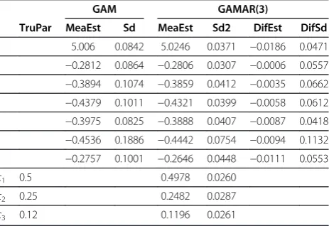
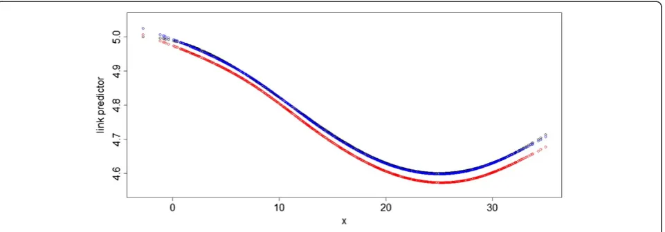
In Figure 5, we can see the mean estimated temperature effects from GAMAR(3) is closer to the true effect than that from GAM. Meanwhile, the Pearson correlation coficients between estimated temperature effect and true ef-fect are also different (GAM: 0.9341; GAMAR(3): 0.9980), which means GAMAR(3) provides a better fit. Also, the standard deviations of estimates from GAM are larger than those from GAMAR (Table 2).

Table 1 Results from GAM, GAMM, GAMAR(3) in simulation study 1

GAM GAMM (AR(3) correlation structure) GAMAR(3)

TruPar MeaEst Bias RelErr Coverage Coverage2 MeaEst Bias RelErr Coverage MeaEst Bias RelErr Coverage β0 5.02 4.9991 −0.0209 0.0127 38 58.8 5.0065 −0.0135 0.0049 92 5.0182 −0.0018 0.0055 94.8

β1 −0.35 −0.3574 −0.0074 0.1922 33.5 52.4 −0.3576 −0.0076 0.0757 88 −0.3561 −0.0061 0.0686 93.9

β2 −0.36 −0.3672 −0.0072 0.229 35.3 56.4 −0.3662 −0.0062 0.0843 96 −0.362 −0.002 0.0885 94.6

β3 −0.38 −0.382 −0.002 0.1531 34.2 55.3 −0.3787 0.0013 0.0608 96 −0.3757 0.0043 0.0733 93.8

β4 −0.33 −0.3281 0.0019 0.428 38.6 62.6 −0.3418 −0.0118 0.1329 98 −0.3262 0.0038 0.1604 95.5

β5 −0.15 −0.1495 0.0005 0.4924 35.4 55.0 −0.1581 −0.0081 0.202 92 −0.1472 0.0028 0.2201 93.8 Mea_co 0.0067 0.2512 35.8 56.8 –0.0077 0.0934 93.7 0.0035 0.1027 94.4

c1 0.5 0.4982 −0.0018 0.0422 95.3

c2 0.25 0.2477 −0.0023 0.0947 93.4

c1 0.12 0.1197 −0.0003 0.1737 94.7

Mea_ar 0.0015 0.1035 94.5

TruPar=True Parameters=βiorci. MeaEst=Mean estimates=―_β^or―c^i. Bias=―_βi^―βior―c^i―ci.

RelErr=Relative Error=β^iβi

=βi

orjð^ciciÞ=cij.

Coverage: the percentage ofestimated 95%CI whichcovers true coefficient in all estimated 95%CI. Coverage2: coverage from GAM which accounts for overdispersion.

Mea_co: Mean absolute Bias, RelErr, Coverage for parameters of covariates. Mea_ar: Mean absolute Bias, RelErr, Coverage for parameters of AR terms.

Table 2 Results from GAM and GAMAR(3) in simulation study 2

GAM GAMAR(3)

TruPar MeaEst Sd MeaEst Sd2 DifEst DifSd

5.006 0.0842 5.0246 0.0371 ₋0.0186 0.0471

−0.2812 0.0864 −0.2806 0.0307 −0.0006 0.0557

−0.3894 0.1074 −0.3859 0.0412 −0.0035 0.0662

−0.4379 0.1011 −0.4321 0.0399 −0.0058 0.0612

−0.3975 0.0825 −0.3888 0.0407 −0.0087 0.0418

−0.4536 0.1886 −0.4442 0.0754 −0.0094 0.1132

−0.2757 0.1001 −0.2646 0.0448 −0.0111 0.0553

c1 0.5 0.4978 0.0260 c2 0.25 0.2482 0.0287 c3 0.12 0.1196 0.0261

Application to temperature-mortality research

In the real case analysis, GAM is first used. The long time trend of original observations is unobvious as shown in the left side of Figure 6. So a rather small df: 2, is used to control this secular trend. The daily mortality after adjustment is in the right side of Figure 6.

And the complete GAM is given below:

EðytÞ ¼μt¼ expðηtÞ

ηt¼β0þnsðtÞ þnsðtemptlag1Þ

þnsðtemptlag2Þ þnsðprestÞ þnsðhumitÞ

þnsðno2tÞ þnsðso2tÞ þnsðpm10tÞ

þwtðweektÞ ð7Þ Lagged days of two temperature terms and df of all remaining natural spline functions are first determined in a sequence to minimize AIC. Then this set of meters is used as starting value to find the final para-meters which minimize AIC locally. The final parapara-meters are:lag1 = 4,lag2 = 10, dftempt₋lag1= 5, dftempt−lag2= 4, dfpres = 2, dfhumi = 2, dfno2 = 3, dfso2 = 2, dfpm10 = 3

The two lagged temperature terms separately repre-sent short term temperature effect and long term

temperature effect. The termwtðweektÞ ¼ X6

i¼1

βiIiðweektÞ stands for week effect, whereweektrepresents corresponding

day in a week for date t, andIi(weekt),i= 1,2,3,4,5,6 are in-dicator functions for the number of a day in a week. For each function, if weekt = i, Ii (weekt) = 1; if weekt ≠ i, Ii (weekt) = 0.

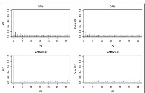
Figure 7 shows that PACF all exceed 95% CI bounds for the autocorrelations (blue dashed line) [38] lags less than 5, and are contained within the bounds for lags lar-ger than 4. So GAMAR(4) is then chosen to fit the data Figure 3ACF and PACF of GAM and GAMAR(3) for Sample 1 from simulation study 2.These statistics are calculated on Pearson residuals zt¼^ytffiffiffiyt

^ yt

p from both models.

Figure 4The temperature effects in link scale for Sample 1

as described below:

EðytÞ ¼μt¼ expðηtÞ ηt¼fðxtÞ þ

X4

i¼1

ci ln yti

ηti

fðxtÞ ¼βtþnsðtÞ þnsðtempt4Þ þnsðtempt10Þ

þnsðprestÞ þnsðhumitÞ þnsðno2tÞ

þnsðso2tÞ þnsðpm10tÞ þwtðweektÞ

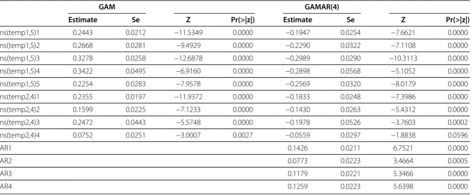
ð8Þ All ACF and PACF of Pearson residuals from (8) are now below 0.1, thus Pearson residuals from GAMAR(4) are close to white noise. The estimated coefficients of two lagged temperature terms and AR terms are given in Table 3. In Figure 8 and Figure 9, we can see that the estimated effects of tempt-4, tempt-10 from two models are different.

Discussion

In environmental epidemiological studies, the meteoro-logical/environmental influences on human health indi-cators are often explained in a modelling framework. And the predominately used models are GLM/GAM. In our research, the drawbacks of GLM/GAM are studied, and their melioration: GAMAR, is given. Simulation studies reveal that GAMAR is more suitable when observations are autocorrelated.

While the true AR order is known in simulation studies, AR order needs to be determined in real case. Three enlightening perspectives into this issue are given below:

1. In time series analysis, ACF and PACF are good indicators of the order of process. CIs of an uncorrelated series are often treated as criterion for selecting orders [38]. For example, when PACF exceed the limit of CI at certain lag, autoregressive

term at that lag needs to be modelled. This approach is used to preliminarily determine the AR order in the real case study.

2. Significance of AR terms can also be considered in modelling. If p-value of AR(n0+1) from GAMAR

(n0+1) is larger than 0.05, while p-value of AR(n0)

from GAMAR(n0) is less than 0.05, then GAMAR

(n0+1) is unnecessary and GAMAR(n0) is a

favorable model. To illustrate it, we also use GAMAR(5) to the real data, and find p-value of AR(5) to be 0.1460>0.05.

3. The goal of introducing AR terms is to control autocorrelation. So if Pearson residuals of GAMAR (n0) show little sign of autocorrelation, or the PACF

is within the CI for all lags, then the AR terms are adequate. In real data case, this requirement is justified.

In application, the first and second advices are prac-tical methods to determine AR order preliminarily, and the third can be used to finally justify the choice. There have been extensive discussions about choosing AR orders [39].

We also want the covariate parameter estimation to be robust with respect to different AR orders. Simulation study provides some information for this issue: while the real model is GAMAR(3) in simulation study 1. GAMAR(1), GAMAR(2), GAMAR(4), GAMAR(5) are also used for estimation. From Table 1 in Additional file we can see that GAMAR(1), GAMAR(2) fit data much better than GAM; while they differ little from GAMAR (3). Since the true AR(3) parameter is rather small (0.12), probably when the effect of neglected AR term is small, covariate parameter estimation won’t differ much. When the AR order is larger than the real, the estima-tion results are almost the same as GAMAR(3). In all, Figure 5The averaged temperature effects in link scale from Simulation study 2.Black: the true effect, Red:nsðx= =;6Þfrom GAM, Blue:

= =

Figure 7ACF and PACF of GAM and GAMAR(4) for real case.These statistics are calculated on Pearson residualszt¼^ytffiffiffiyt ^ yt

p from both models.

covariate parameter estimation is robust with respect to disturbance of AR order.

GAMM can also give good estimates as shown in Table 1. However, while the speed of GAMM in fitting short time series is acceptable, say 2.05 seconds for sam-ple with 100 observations and 10.17 seconds for samsam-ple with 200 observations (both executed in server), the time grows nonlinearly with respect to the length of time series and thus GAMM would become computa-tionally formidable when time series data is long. For ex-ample, one sample of 1461 observations in simulation study 1 would take about 1 hour and 7 minutes for GAMM, while only 0.02 seconds for GAMAR (both exe-cuted in server): the former is 2×105 times the latter. Thus GAMM is much more computing intensive than

GAMAR when sample size is large. Therefore, we only calculated 50 samples for GAMM in simulation study 1.

While we use natural cubic spline as smoother in the model, penalized spline and smoothing spline can also be implemented. With natural splines, one constructs a spline basis with knots at fixed locations throughout the range of the data. Smoothing splines and penalized splines have circumvented the problem of choosing the knot locations by constructing a very large spline basis and then penalizing the spline coefficients to reduce the effective number of df [40]. Despite the flexibility the penalized way provided, [40] identified both fully para-metric and nonparapara-metric methods can perform well in similar studies. Thus natural spline smoother can still address many practical problems. In addition, our model

Figure 8Effects oftempt−4.Black:

= = = =

nsðtempt4;6Þfrom GAM, Red:

= = = =

nsðtempt4;6Þfrom GAMAR(4). Figure 9Effects oftempt−10.Black:

= = = =

nsðtempt10;6Þfrom GAM,

Red:nsðtempt= = = =10;6Þfrom GAMAR(4). Table 3 temperature effects and AR estimates from GAM and GAMAR(4)

GAM GAMAR(4)

Estimate Se Z Pr(>|z|) Estimate Se Z Pr(>|z|)

ns(temp1,5)1 0.2443 0.0212 ₋11.5349 0.0000 ₋0.1947 0.0254 ₋7.6621 0.0000 ns(temp1,5)2 0.2668 0.0281 −9.4929 0.0000 −0.2290 0.0322 −7.1108 0.0000 ns(temp1,5)3 0.3278 0.0258 −12.6878 0.0000 −0.2989 0.0290 −10.3113 0.0000 ns(temp1,5)4 0.3422 0.0495 −6.9160 0.0000 −0.2898 0.0568 −5.1052 0.0000 ns(temp1,5)5 0.2254 0.0283 −7.9578 0.0000 −0.2569 0.0320 −8.0179 0.0000 ns(temp2,4)1 0.2355 0.0197 −11.9372 0.0000 −0.1833 0.0248 −7.3986 0.0000 ns(temp2,4)2 0.1599 0.0225 −7.1233 0.0000 −0.1430 0.0263 −5.4312 0.0000 ns(temp2,4)3 0.2472 0.0443 ₋5.5748 0.0000 ₋0.1978 0.0526 ₋3.7603 0.0002 ns(temp2,4)4 0.0752 0.0251 −3.0007 0.0027 −0.0559 0.0297 −1.8838 0.0596

AR1 0.1426 0.0211 6.7521 0.0000

AR2 0.0773 0.0223 3.4664 0.0005

AR3 0.1179 0.0221 5.3466 0.0000

AR4 0.1259 0.0223 5.6398 0.0000

Estimate: estimate for a parameter. Se: Standard Error for a parameter.

Z=Estimate/Se, which approximately follows N(0,1).

can be straightforwardly extended to the nonparametric way by including the penalty.

For natural spline with B-spline basis, selecting the df is of essential importance for application. A general ap-proach is to use a data-driven method and to select the number of df which optimizes a particular criterion [40], like AIC. We used AIC to determine df of all splines ex-cept that of time in the real case. Another strategy is to use a df based on background knowledge or previous studies. For example, natural spline of time is chosen to represent the long term trend among different years, and itself shouldn’t contain any yearly fluctuation. Whether df meets the requirement is judged by compar-ing the trend of observations before and after adjust-ment, as well as the shape of the spline function visually in Figure 6. Section 2.1 of [40] gives a full treatment of this issue.

Besides including lagged temperature effects addi-tively in the model, [41,42] have developed a family of distributed lag non-linear models (DLNM), which can simultaneously represent non-linear exposure-response dependencies and delayed effects. Still, AR terms can be aptly added to DLNM just as what we’ve done to GAM.

Finally, the model can also be applied in other areas. Researchers can use GAMAR for their specific research purposes. The most immediate extensions are other en-vironmental epidemiological studies, specifically studies quantifying relationships between air pollution and mor-tality. Air pollution functions in a different way from temperature to impact human health, and there are also some differences between their modelling: 1) the air pollution-mortality relation is often simplified as linear, for such simplicity facilitates parameter estimation and interpretation; 2) distributed lag model is often used, since the effects of air pollution can last for many days; 3) cumulative effect: the total impact of pollution of a certain day over a period of following days, represented by the sum of parameters at all lags, is of great interest [9]. Such differences pose new questions for further study, like assessing the impact of AR terms on esti-mated cumulative effect rather than a single parameter.

Conclusions

This article proposes GAMAR for fitting time series data with explanatory variables and autoregressive terms. Two simulation studies with functions that approximate the response from the real example showed that GAMAR performed better than GAM. In the real ex-ample, there was residual autocorrelation with GAM, but little sign of autocorrelation with GAMAR. Also, dif-ferent estimates of the temperature effects were obtained with GAMAR and GAM.

Appendix

Modified Newton’s method

Given partial likelihood, maximum partial likelihood estimators are solved by a modified Newton’s method. For Newton’s method, the iteration goes:

θmþ1¼θm ∂

2_{lnð ÞPL} ∂θi∂θj

1

∂lnð ÞPL ∂θ jθ¼θm; until convergence.

For a modified Newton’s method, the iteration goes:

θmþ1¼θmþΓ1ð Þθm ∂ lnð ÞPL

∂θ jθ¼θm; ð9Þ

until it convergence.

Here Γ θð Þ ¼ ∂2_∂ln_θ∂ð Þ_θPLT , which is the information matrix, andΓ*−1(θm) is a modified version ofΓ−1(θm).

In (9):

∂lnð ÞPL

∂θi ¼

∂Xn

t¼1

ðytlnð Þ μt μt lnð ÞÞyt!

∂θi

¼Xn

t¼1

ytμt

ð Þ∂ηt

∂θi;

Γ θð Þ ¼

∂Xn

t¼1 ytμt

ð Þ∂ηt

∂θi

∂θj ¼

A B

BT _C

:

Since lnð Þ ¼μ_t η_t ¼X m

i¼1

βiXtiþ Xp

j¼1

cj ln ytj

Xm

i¼1

βiXtj;i

, then:

∂ηt

∂βi

¼Xti Xp

r¼1

crXtr;i;∂_∂ηt

ci ¼

lny_tiX

m

k¼1

βkXti;k;

∂2_η

t

∂βi∂βj

¼0; ∂

2_η

t

∂ci∂cj¼ 0; ∂

2_η

t

∂βi∂cj¼

Xtj;i:

So

A¼ X

n

t¼1

μtðXti Xp

r¼1

crXtr;iÞðXtj Xp

r¼1

crXtr;jÞ !

mm ;

B¼ X

n

t¼1

μtðXti Xp

r¼1

crXtr;iÞ ln ytj

Xm

k¼1

βkXtj;k

þðytμtÞXtj;i !!

mp;

C¼ X

n

t¼1

lny_tiX

m

k¼1

βkXti;k !

ln y_tj

Xm

k¼1

βkXtj;k !!

And the modified inverse matrixΓ*−1(θm) is defined as: ifΓ(θ) is reversible, thenΓ*−1(θ) =Γ−1(θ);

If Γ(θ) is irreversible. And its eigenvalue are λ1,

λ2,. . .,λmp, then we can find orthogonal matrix P, which satisfies:

PT_{Γ θð ÞP¼diag λ}

1;. . .;λmp

:

Letλi*= max(λi,δ),δ= 0.01,i= 1, 2,⋯,mp, then:

Γ1

ð Þ ¼θ Pdiag λ11;. . .;λmp1

PT:

Such procedure ensures Γ*−1(θm) to be positive definite.

Additional files

Additional file 1:R code for this study.This file contains core R codes for this study, including the function of GAMAR, data generation in simulation studies, data fitting in simulation studies, real case analysis (including the procedure to choose the parameters) and generation of tables and figures. This file also contains a brief description of every R program.

Additional file 2:Additional Tables.This file contains 2 tables related to simulation study 1.

Competing interests

The authors declare that they have no competing interests.

Authors’contributions

LY conducted the analysis and drafted the manuscript. GQ participated in discussions and provided advice. NZ inspired and tutored LY, and reviewed the paper. CW and GS collected the mortality data for real case study. All authors read and approved the final manuscript.

Acknowledgements

This research is supported by a project 30972551 from National Natural Science Foundation of China (NSFC).

Author details

1

Department of Biostatistics, School of Public Health, Fudan University, Shanghai, China.2_{Vital Statistics Division, Shanghai Municipal Center for} Disease Control & Prevention, Shanghai, China.

Received: 30 January 2012 Accepted: 9 October 2012 Published: 30 October 2012

References

1. Ellis FP, Nelson F:Mortality in the elderly in a heat wave in New York City, August 1975.Environ Res1978,15:504–512.

2. McKee CM:Deaths in winter: can Britain learn from Europe?Eur J Epidemiol1989,5(2):178–182.

3. Ballester F, Corella D, Perez-Hoyos S, Saez M, Hervas A:Mortality as a function of temperature. A study in Valencia, Spain, 1991–1993.Int J Epidemiol1997,26(3):551–561.

4. Ha J, Shin Y, Kim H:Distributed lag effects in the relationship between temperature and mortality in three major cities in South Korea.Sci Total Environ2011,409(18):3274–3280.

5. Yu W, Guo Y, Ye X, Wang X, Huang C, Pan X, Tong S:The effect of various temperature indicators on different mortality categories in a subtropical city of Brisbane, Australia.Sci Total Environ2011,409(18):3431–3437. 6. Basu R, Malig B:High ambient temperature and mortality in California:

Exploring the roles of age, disease, and mortality displacement.Environ Res2011,111(8):1286–1292.

7. Patz JA, Engelberg D, Last J:The effects of changing weather on public health.Annu Rev Publ Health2000,21:271–307.

8. Baker DANM:Environmental Epidemiology: Study Methods and Application. Oxford: Oxford University Press; 2008.

9. Peng RD, Dominici F:Statistical methods for environmental epidemiology in R. New York: Springer; 2008.

10. Ostro BD, Roth LA, Green RS, Basu R:Estimating the mortality effect of the July 2006 California heat wave.Environ Res2009,109(5):614_–619. 11. Hertel S, Le Tertre A, Jockel KH, Hoffmann B:Quantification of the heat

wave effect on cause-specific mortality in Essen, Germany.Eur J Epidemiol2009,24(8):407–414.

12. Goldberg MS, Gasparrini A, Armstrong B, Valois MF:The short-term influence of temperature on daily mortality in the temperate climate of Montreal, Canada.Environ Res2011,111(6):853–860.

13. Hajat S, Kovats RS, Atkinson RW, Haines A:Impact of hot temperatures on death in London: a time series approach.J Epidemiol Community Health 2002,56(5):367–372.

14. Ballester J, Robine JM, Herrmann FR, Rodo X:Long-term projections and acclimatization scenarios of temperature-related mortality in Europe.Nat Commun2011,2:358.

15. McCullagh P, Nelder JA:Generalized Linear Models. London: Chapman and Hall/CRC; 1989.

16. Hastie TJ, Tibshirani RJ:Generalized Additive Models. London: Chapman and Hall/CRC; 1990.

17. Braga AL, Zanobetti A, Schwartz J:The effect of weather on respiratory and cardiovascular deaths in 12 U.S. cities.Environ Health Perspect2002, 110(9):859–863.

18. Carson C, Hajat S, Armstrong B, Wilkinson P:Declining vulnerability to temperature-related mortality in London over the 20th century.Am J Epidemiol2006,164(1):77–84.

19. Muggeo VM:Modeling temperature effects on mortality: multiple segmented relationships with common break points.Biostatistics2008, 9(4):613–620.

20. Kim H, Ha JS, Park J:High temperature, heat index, and mortality in 6 major cities in South Korea.Arch Environ Occup Health2006,61(6):265–270. 21. Curriero FC, Heiner KS, Samet JM, Zeger SL, Strug L, Patz JA:Temperature

and mortality in 11 cities of the eastern United States.Am J Epidemiol 2002,155(1):80–87.

22. Ren C, Williams GM, Morawska L, Mengersen K, Tong S:Ozone modifies associations between temperature and cardiovascular mortality: analysis of the NMMAPS data.Occup Environ Med2008,65(4):255–260.

23. Hoffmann B, Hertel S, Boes T, Weiland D, Jockel KH:Increased cause-specific mortality associated with 2003 heat wave in Essen, Germany. J Toxicol Environ Health A2008,71(11_–12):759_–765.

24. Anderson BG, Bell ML:Weather-related mortality: how heat, cold, and heat waves affect mortality in the United States.Epidemiology2009, 20(2):205_–213.

25. Schwartz J:The distributed lag between air pollution and daily deaths. Epidemiology2000,11(3):320–326.

26. Hamilton JD:time series analysis. Princeton, NJ: Princeton University Press; 1994.

27. Kutner M, Nachtsheim C, Neter J, Li W:Applied Linear Statistical Models Fifth Edition. New York: McGraw-Hill/Irwin; 2005.

28. Barron DN:The analysis of count data: overdispersion and autocorrelation.Sociol Methodol1992,22:179–220.

29. Zeger SL, Liang KY:Longitudinal data analysis for discrete and continuous outcomes.Biometrics1986,42(1):121–130.

30. Liang KY, Zeger SL:Longitudinal data analysis using generalized linear models.Biometrika1986,73(1):13_–22.

31. Pinheiro JC, Bates DM:Mixed-Effects Models in S and S-plus. New York: Springer; 2000.

32. Wood SN:Generalized Additive Model: an introduction with R. New York: Chapman and Hall/CRC; 2006.

33. Lin X:SAS Macro GAMM1 to fit generalized additive mixed models using smoothing splines.: Harvard University; http://scholarjsagotskydev.iq.harvard. edu/amaity/software/gamm1.

34. The GLIMMIX Procedure.: SAS Institute inc; 2006. support.sas.com/rnd/app/ papers/glimmix.pdf.

35. Benjamin MA, Rigby RA, Stasinopoulos DM:Generalized autoregressive moving average models.J Am Stat Assoc2003,98(461):214_–223. 36. Cox DR, Gudmundsson G, Lindgren G, Bondesson L, Harsaae E, Laake P,

37. Ruoyan M:Estimation of Dispersion Parameters in GLMs with and without Random Effects.: Stockholm University; 2004. http://www2.math.su.se/ matstat/reports/serieb/2004/rep5/report.pdf.

38. Box G, Jenkins GM, Reinsel G:Time Series Analysis: Forecasting & Control. 3rd edition.: Prentice Hall; 1994.

39. Zhang S, Qi L:shi jian xu lie fen xi jian ming jiao cheng. Beijing: Beijing jiaotong university press; 2003.

40. Peng RD, Dominici F, Louis TA:Model choice in time series studies of air pollution and mortality.J R Stat Soc A Stat Soc2006,169(2):179–203. 41. Gasparrini A, Armstrong B, Kenward MG:Distributed lag non-linear

models.Stat Med2010,29(21):2224–2234.

42. Gasparrini A:Distributed lag linear and non-linear models in R: The package dlnm.J Stat Softw2011,43(8):1–20.

doi:10.1186/1471-2288-12-165

Cite this article as:Yanget al.:Using a generalized additive model with autoregressive terms to study the effects of daily temperature on mortality.BMC Medical Research Methodology201212:165.

Submit your next manuscript to BioMed Central and take full advantage of:

• Convenient online submission

• Thorough peer review

• No space constraints or color figure charges

• Immediate publication on acceptance

• Inclusion in PubMed, CAS, Scopus and Google Scholar

• Research which is freely available for redistribution