A Generalization of Two-Parameter Lindley Distribution with Properties and Applications

(1)

A Generalization of Two-Parameter Lindley Distribution

with Properties and Applications

Rama Shanker1,*, Kamlesh Kumar Shukla1, Tekie Asehun Leonida2

1

Department of Statistics, Eritrea Institute of Technology, Asmara, Eritrea 2

Department of Applied Mathematics, University of Twente, The Netherlands

Abstract

In this paper, a generalization of two-parameter Lindley distribution (GTPLD), which includes one parameter exponential and Lindley distributions, two-parameter Lindley distribution (TPLD) of Shanker and Mishra (2013), Weibull distribution, gamma distribution, generalized gamma distribution of Stacy (1962) and power Lindley distribution of Ghitany

et al (2013) as particular cases, has been proposed. Its moments, hazard rate function, mean residual life function, order statistic, Renyi entropy measure has been studied. Method of maximum likelihood estimation has been discussed for estimating its parameters. Applications of the distribution have been explained with two examples of observed real lifetime datasets.

Keywords

Two-parameter Lindley distribution, Moments, Hazard rate function, Mean residual life function, Order statistic, Renyi entropy measure, Maximum likelihood estimation, Applications

1. Introduction

Shanker and Mishra (2013) introduced a two-parameter Lindley distribution (TPLD) defined by its probability density function (pdf) and cumulative distribution function (cdf)



; ,



2





; 0, 0, 1

1



     

 y

f y    y e  x   

  (1.1)



; ,



1 1 ; 0, 0, 1

1 

 

  _ _    



 

y x

F y   e  x   

  (1.2) The pdf (1.1) can be expressed as



; ,



 1



;

 

 1

 

2 ; 2,



f y  p g y p g y 

where

1 



p  

  ,





1 ; ; 0, 0



 y  

g y e  y 





2

2 ;   y ; 0, 0

g y  y e  y  .

Clearly the density (1.1) is a two-component mixture of an exponential distribution with scale parameter  and a gamma distribution with shape parameter 2 and scale parameter , with mixing proportion

1 



p  

  . Shanker and Mishra (2013)

studied its various properties including coefficients of variation, skewness, kurtosis; hazard rate function, mean residual life

* Corresponding author:

shankerrama2009@gmail.com (Rama Shanker) Published online at http://journal.sapub.org/ijps

(2)

function and stochastic ordering. The estimation of its parameters using both the maximum likelihood estimation and the method of moments along with applications of TPLD to model lifetime data has also been discussed by Shanker and Mishra (2013). It can be easily shown that Lindley distribution, introduced by Lindley (1958), having pdf



;



2



1



; 0, 0

1



   



y

f y  y e  x 

 (1.3) is a particular case of TPLD (1.1) at  1_{. Lindley distribution has been studied in detail by Ghitany et al (2008). Shanker et}

al (2015) have detailed and critical study on applications of exponential and Lindley distribution for modeling real lifetime data from biomedical sciences and engineering and observed that both exponential and Lindley are competing each other. Shanker et al (2016) have discussion on applications of gamma distribution and Weibull distribution for real lifetime data from engineering and biological sciences. Shanker (2016) has discussed various important statistical properties including coefficient of variation, skewness, kurtosis and index of dispersion along with various applications of generalized Lindley distribution (GLD) introduced by Zakerzadeh and Dolati (2009). Shanker and Shukla (2016) have detailed comparative study on applications of three-parameter generalized gamma distribution (GGD) and generalized Lindley distribution (GLD) and observed that these two distributions are competing each other for modeling lifetime data.

In this paper, an attempt has been made to derive a generalization of two-parameter Lindley distribution (GTPLD), which includes one parameter exponential and Lindley distributions, two-parameter Lindley distribution (TPLD) of Shanker and Mishra (2013), Weibull distribution, gamma distribution, generalized gamma distribution of Stacy (1962) and power Lindley distribution of Ghitany et al (2013) as particular cases. The moments, hazard rate function, mean residual life function, order statistic and Renyi entropy measure of the distribution have been studied. Method of maximum likelihood estimation has been discussed for estimating its parameters. Applications of the distribution have been explained with two examples of observed real lifetime datasets and its goodness of fit has been compared with other lifetime distributions.

2. A Generalization of Two-Parameter Lindley Distribution

Assuming the power transformation _ 1

X Y in (1.1), the pdf of Xcan be obtained as





2 1





1 ; , , ; 0, 0, 0, 1

1

 

      



x

f x     x  x e   x    

  (2.1)



 



1 ; , 1 2 ; 2, ,

p g x   p g x   , (2.2) where,

1 

2,



and scale parameter , with mixing

proportion

1 



p  

  . At 1 and  1, (2.1) reduces to the Lindley distribution (1.3). At  1, (2.1) reduces to the

Power Lindley distribution introduced by Ghitany et al (2013) having pdf





2 1





2 ; , 1 ; 0, 0, 0

1

 

    



x

f x    x x e   x  

 (2.3) The gamma

 

2, distribution and a generalized gamma



2, , 



distribution are also particular cases of (2.1) for



0,1



and  0 respectively. It can be easily shown that (2.1) reduces to Weibull distribution for  . Further, for 1 and  , (2.1) reduces to exponential distribution.

(3)





1 ; , , 1 1 ; 0, 0, 0, 1

1



 

   _      

 

 

x

F x e x

 _ 



      

  (2.4)

We use X ~ GTPLD



  , ,



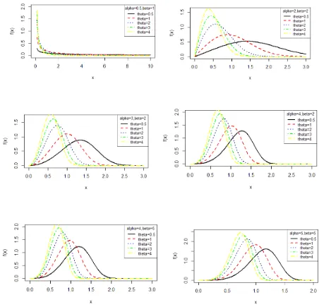
to denote a random variable having GTPLD (2.1) with parameters ,  and  having pdf (2.1) and cdf (2.4).

The behavior of the pdf and the cdf of GTPLD have been shown graphically for varying values of parameters ,  and  in figures 1 and 2 respectively.

(4)

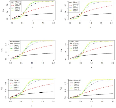
Figure 2. Behavior of the cdf of GTPLD for varying values of parameters  , and 

3. Reliability Properties

3.1. Survival Function and Hazard Rate Function The survival function of GTPLD can be expressed as



; , ,



1



; , ,



1 ; 0, 0, 0, 1

1



 

    _      

 

 

x

S x F x e x

 _ 



         

  .

Thus the hazard rate function of GTPLD can be obtained as







_

_











2 1

; , ,

; , , ; 0, 0, 0, 1

; , , ₁

 _

      

 

x x

f x

h x x

S x _x

 



  

  

      

   _{ } _ .

(5)

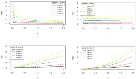
Figure 3. Behavior of the hazard rate function of GTPLD for varying values of parameters  , , and  3.2. Mean Residual Life Function

The mean residual life function, m x



; , ,  



of GTPLD (2.1) can be obtained as





_

1

_





; , , ; , ,

; , , 



_



x

m x t f t dt x

S x

     

  





2

1



 

  

 _ _ 

 



t

x x

t t e dt x

x e

    

 

  _

  

2

2 1

u



u

x

x x

m x e u du e u du x

x e

 _  _ 

  _ _



   

  

2

1 1

1 2

1 1

1, 2,

1   

 _ _  _ _ 

   

 _ _ _ _

 

  

 

 _ _ 

 

  x _ _

x x

x

x e

 



 

 

 

 _  

(6)

1

1 1

1, 2,

1 

   

_  _ _  _

   

 

 _ _ 

  x

x x

x

x e

 



 



   

 

   

.

It can be easily verified that



 







1

2 1

1 1 0; , ,

1

   

  _{ } _

 



m



    

   

  



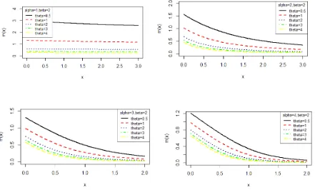
. The behavior of m x



; , ,  



of GTPLD for varying values of parameters , , and   are shown in figure 4

Figure 4. Behavior of the mean residual life function of GTPLD for varying values of parameters  , , and 

4. Statistical Properties

4.1. Moments

The rth moment about origin, _r of GTPLD (2.1) can be obtained as

 

2





1

0

1 

  

   





r r x

r E X x x e dx



  

 

 

 

2

1 2 1

0 0

1

 

     

 

 

 

 _



_

x r x r

e  x dx e  x  dx

  _

  .

Taking yx, which gives

 

1 

x y  and

1

1 



dx y dy

 

(7)

1 1 2 1 1 2 0 0 1 1 1                     



 r r y y

r e y y dy e y y dy

     _ _  _ _         2 1

2 _{1 1}

0 0 1    _{ }         _  _  _



_ r r y y

e  y dy e  y dy



3 ₂ ₄

4 4 4 1       _{ }               .

The variance of GTPLD can thus be obtained as

 













2 2 2 2

2 2 1 ₂

2 4

2 1

2 2 1

1         _{ }   __{ }_                               .

The higher central moments, if required, can be obtained using the relationship between central moments and raw moments. The skewness and kurtosis measures, upon substituting for the raw moments, can be obtained using the expressions

Skewness

 

3

3 2 1

3

3 2

=

  

  

 and Kurtosis

   

2 4

4 3 1 2 1 1

4

4 6 3

      

     

 .

4.2. Distribution of Order Statistics

(8)

     

! 1

 



₁

 



 

1 ! !

      n k k Y n

f y F y F y f y

k n k



 



 

1

   

0

!

1 1 ! !

        _ _   



_ _ n k

l k l l

n k n

F y f y

l

k n k

and

 



1

 







 

 _{ } 

 



n _j n j

Y

j k

n

F y F y F y

j

 

0 1          _{ } _    

 

n n j l j l

j k l

n n j

F y

j l ,

respectively, for k1, 2, 3,...,n.

Thus, the pdf and the cdf of kth order statistics of GTPLD are given by

 

_

_



_{ }



_

1 2 1 0 ! 1 1

1 1 ! ! 1

    _            _ _   _ _    



  _ _  _ _ k l x _{n k}

x Y

l

n x x e _{n k} _x

f y e

l

k n k

    _      _    

and

 

0

1 1 1

1               _{ } _    _ _        _ _ _ _

 

j l n j n l x Y

j k l

n n j x

F y e

j l

 _ 

  

4.3. Renyi Entropy Measure

An entropy of a random variable X_{is a measure of variation of uncertainty. A popular entropy measure is Renyi entropy}

R

T  f x dx

 where 0 and  1.

Thus, the Renyi entropy for GTPLD (2.1) can obtained as

 





 j x j x

x e dx

j  _             





  2 0 0 1 1 log 1 1   _{ }   _ _ _{ }     __ _ _{ } _  _  _ _{ } 





 j x j j

e x dx

j               _

Taking yx, which gives

 

1



x y  and

1

1 



dx y dy

 

 , we get

 

_

_

  1 2 0 0 1 1 log 1 1    _{ }        _{ }   _ _ _ _            





y j

R _j

j

y

T e y dy

(9)





   1

2 ₁

0 0

1 1

log

1 1

 

 _{ } _

 

_ _ _{ } 

 

 __ _ _{ } _

 _  _ _{ }

 

 





y j

j j

e y dy

j

 _ 

  _

   

    _



  

 

_

_{ }



2 1

1

0

1

1 1

log

1 1

  



_ _ _{ }_ _ _ _ _

 

 _ __ _ _       _

    

 







j

j j



  

  

   _{ } _











 

1 1 1

ln ln 2 ln ln 1 ln 1 ln

  

 _    _



n  _i  



n _i 



n _i

i i i

L n      x  x  x .

The maximum likelihood estimates



  ˆ, ,ˆ ˆ



of parameters



  , ,



of GTPLD (2.1) is the solutions of the following natural log- likelihood equations

1

ln 2

0 1 _

 _ _ _ _

 



n i i

L n n

x 

   

 

_{ }

1 1 1

ln ln

ln ln 0

  

 _ _ _ _ _





_



n n n

i i

i i i

i i i i

x x

L n

x x x

x



 

  _

1

ln 1

0 1 _



   

 





n

i i

L n

x 

   

These three natural log- likelihood equations do not seem to be solved directly because they cannot be expressed in closed forms. However, the MLE’s



  ˆ, ,ˆ ˆ



of parameters



  , ,



can be obtained directly by solving the log likelihood equation using Newton-Raphson iteration method available in R –Software till sufficiently close estimates of ˆ, ˆ and ˆ are obtained.

6. Numerical Examples

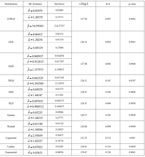
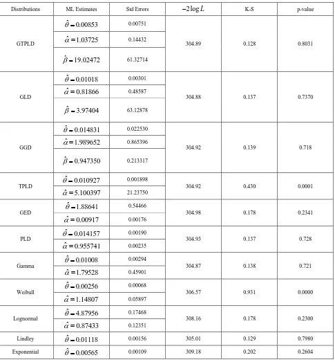
The applications of GTPLD have been explained with two real lifetime datasets regarding failure times (in minutes) from Lawless (2003) pp. 204 and 263. The goodness of fit of GTPLD has been discussed along with the goodness of fit given by generalized Lindley distribution (GLD) introduced by Zakerzadeh and Dolati (2009), generalized gamma distribution introduced by Stacy (1962), two-parameter Lindley distribution of Shanker and Mishra (2013), generalized exponential distribution proposed by Gupta and Kundu (1999), power Lindley distribution introduced by Ghitany et al (2013), gamma distribution, Weibull distribution suggested by Weibull (1951), Lognormal distribution, Lindley distribution and exponential distribution. In table 1, the pdf and the cdf of fitted distributions has been presented. The goodness of fit of the fitted distribution has been presented in tables 2 and 3, respectively.

Dataset 1: The first set of datarepresents the failure times (in minutes) for a sample of 15 electronic components in an accelerated life test and the data are

1.4, 5.1, 6.3, 10.8, 12.1, 18.5, 19.7, 22.2, 23.0, 30.6, 37.3, 46.3, 53.9, 59.8, and 66.2. Dataset 2: The following data set represents the number of cycles to failure for 25 100-cm specimens of yarn, tested at a particular strain level, Lawless (2003) pp. 204 and 263.

(10)

Table 1. The pdf and the cdf of the fitted distributions

Distributions pdf and cdf

GLD

pdf



    



1 1

; , , ; 0, 0, 0, 0

1

 



     

  

x x

f x x e x

 



       

  

cdf







 



 



,

 



; , , 1 ; 0, 0, 0, 0

1



  

     

  

x

x x e

F x x

 

      

     

  

GGD

pdf





 

1

; , ,    ; 0, 0, 0, 0



x

f x x e x

 _

  

 

     



cdf









 

,

; , , , 1 ; 0, 0, 0, 0



     



x

F x x



 

     



PLD

pdf









2

1

; , 1 ; 0, 0, 0

1

 

    



x

f x   x x e   x  



cdf



; ,



1 1 ; 0, 0, 0 1



 

      



 

 

x

F x e x

 _ 



   



GED

pdf









1

; ,  1  x   x; 0, 0, 0

f x    e   e  x  

 ₁ _ex _;_x_0,_0, ₀

Gamma

pdf





 

1

; ,   ; 0, 0, 0



x

f x e x x



 



   



cdf









 

,

; ,  1  ; 0, 0, 0

 x

F x    x  



Lognormal

pdf





2 1 log 2

1

; , ; 0, 0, 0

2



 

  

 

   

x

f x e x

x

 

   



cdf



; ,



 log  ; 0, 0, 0

 

x

F x    x  

(11)

Table 2. ML estimates and summary of goodness of fit for dataset 1

Distributions ML Estimates Std Errors 2logL K-S p-value

GTPLD

ˆ 0.02476

 0.03885

127.94 0.097 0.9962

ˆ 1.20279

 0.33713

ˆ 54.99303

 214.27357

GLD

ˆ 0.06415

 0.02132

128.16 0.095 0.9961

ˆ 1.20258

 0.81310

ˆ 0.08329

 0.27068

GGD

ˆ 0.008937

 0.014654

127.98 0.096 0.9960

ˆ 0.912815

 0.417267

ˆ 1.357973

 0.350075

TPLD

ˆ 0.062325

 0.017145

128.21 0.347 0.0397

ˆ 6.343568

 12.14555

GED ˆ 0.04529

0.01372

128.47 0.108 0.9868

ˆ 1.44347

 0.51301

PLD ˆ 0.097651

0.056373

128.47 0.098 0.9950

ˆ 0.904312

 0.160673

Gamma ˆ 0.05235

0.02066

128.37 0.103 0.9920

ˆ 1.44219

 0.47771

Weibull ˆ 0.01190

0.01124

128.04 0.098 0.9950

ˆ 1.30586

 0.24925

Lognormal

ˆ 2.93059

 0.26472

131.23 0.312 0.045

ˆ 1.02527

 0.18718

(12)

Table 3. ML estimates and summary of goodness of fit for dataset 2

Distributions ML Estimates Std Errors 2logL K-S p-value

GTPLD

ˆ 0.00853

 0.00751

304.89 0.128 0.8031

ˆ 1.03725

 0.14432

ˆ 19.02472

 61.32714

GLD

ˆ 0.01018

 0.00301

304.88 0.137 0.7370

ˆ 0.81866

 0.48587

ˆ 3.97404

 63.12878

GGD

ˆ 0.014831

 0.022530

304.92 0.139 0.718

ˆ 1.989652

 0.865396

ˆ 0.947350

 0.213317

TPLD

ˆ 0.010927

 0.001898

304.92 0.430 0.0001

ˆ 5.100397

 21.23750

GED ˆ 1.88641

0.54466

304.98 0.178 0.2341

ˆ 0.00917

 0.00176

PLD ˆ 0.014157

0.00190

304.93 0.137 0.728

ˆ 0.955741

 0.00235

Gamma ˆ 0.01008

0.00294

304.87 0.138 0.721

ˆ 1.79528

 0.45901

Weibull ˆ 0.00256

0.00068

306.57 0.931 0.0000

ˆ 1.14807

 0.05897

Lognormal

ˆ 4.87956

 0.17468

308.16 0.178 0.2300

ˆ 0.87433

 0.12351

Lindley ˆ 0.01118 0.00156 305.01 0.129 0.7980 Exponential ˆ 0.00565 0.00109 309.18 0.202 0.2604

It is obvious from the goodness of fit of GTPLD that GTPLD is competing well with other lifetime distributions and hence can be considered an important lifetime distribution in statistics literature. The variance-covariance matrix of the estimated parameters of the GTPLD for datasets 1 and 2 has been given in tables 4 and 5, respectively.

Table 4. Variance-covariance matrix of GTPLD for dataset 1

ˆ _ˆ ˆ

  

ˆ 0.00176 0.01337 5.19676 ˆ 0.01337 0.10684 36.88400 ˆ 5.19676 36.88400 18207.39274

 

 

_ 

 

 

 

(13)

Table 5. Variance-covariance matrix of GTPLD for dataset 2

ˆ _ˆ ˆ

  

ˆ 0.000056 0.001058 0.380728 ˆ 0.001058 0.020828 6.632788 ˆ 0.380728 6.632788 3761.01813

 

 

_ 

 

 

 

  

7. Concluding Remarks

A generalization of two-parameter Lindley distribution (GTPLD), which includes one parameter exponential and Lindley distributions, two-parameter Lindley distribution (TPLD) of Shanker and Mishra (2013), Weibull distribution, gamma distribution, generalized gamma distribution of Stacy (1962) and power Lindley distribution of Ghitany et al (2013) as particular cases, has been proposed. Its raw moments, hazard rate function, mean residual life function, order statistic, Renyi entropy measure has been studied. Maximum likelihood estimation has been discussed for estimating its parameters. Applications of the distribution have been explained with two examples of observed real lifetime datasets from engineering and the goodness of fit is quite satisfactory over other one parameter, two-parameter and three-parameter lifetime distributions. .

ACKNOWLEDGEMENTS

Authors are grateful to the editor-in-chief and the anonymous reviewer whose comments improved the quality and the presentation of the paper.

REFERENCES

[1] Ghitany, M.E., Atieh, B. and Nadarajah, S. (2008): Lindley distribution and its Application, Mathematics Computing and Simulation, 78, 493 – 506.

[2] Ghitany, M.E., Al-Mutairi, D.K., Balakrishnan, N., and Al-Enezi, L.J. (2013): Power Lindley distribution and Associated Inference,

Computational Statistics and Data Analysis, 64, 20 – 33.

[3] Gupta, R.D. and Kundu, D. (1999): Generalized Exponential Distribution, Austalian & New Zealand Journal of Statistics, 41(2), 173 – 188.

[4] Lawless, J.F. (2003): Statistical Models and Methods for Lifetime Data, Wiley, New York.

[5] Lindley, D.V. (1958): Fiducial distributions and Bayes’ Theorem, Journal of the Royal Statistical Society, Series B, 20, 102 – 107. [6] Renyi, A. (1961): On measures of entropy and information, in proceedings of the 4th berkeley symposium on Mathematical Statistics

and Probability, 1, 547 – 561, Berkeley, university of California press.

[7] Shanker, R. and Mishra, A. (2013): A Two-Parameter Lindley Distribution, Statistics in Transition new Series, 14(1), 45-56. [8] Shanker, R., Hagos, F, and Sujatha, S. (2015): On modeling of Lifetimes data using exponential and Lindley distributions, Biometrics

& Biostatistics International Journal, 2(5), 1-9.

[9] Shanker, R. (2016): On generalized Lindley distribution and its applications to model lifetime data from biomedical science and engineering, Insights in Biomedicine, 1(2), 1 – 6.

[10] Shanker, R. and Shukla, K.K. (2016): On modeling of lifetime data using three-parameter Generalized Lindley and Generalized Gamma distributions, Biometrics & Biostatistics International Journal, 4(7), 1 – 7.

[11] Shanker, R., Shukla, K.K., Shanker, R. and Tekie, A.L. (2016): On modeling of Lifetime data using two-parameter Gamma and Weibull distributions, Biometrics & Biostatistics International journal, 4(5), 1 – 6.