Volume 7, Number 2, pp. 15–23. http://www.scpe.org c 2006 SWPS
HEURISTIC LOAD BALANCING FOR CFD CODES EXECUTED IN HETEROGENEOUS COMPUTING ENVIRONMENTS
DANA PETCU∗, DANIEL VIZMAN†, AND MARCIN PAPRZYCKI‡
Abstract. A graph partitioning-based heuristic load-balancing algorithm known as the Largest Task First with Minimum Finish Time and Available Communication Costs is modified to take into account the dynamic nature and heterogeneity of current large-scale distributed computing environments, like Grids. The modified algorithm is applied to facilitate load balancing of a known CFD code used to model crystal growth.
Key words. load balancing, grid and cluster computing, computational intensive problems
1. Introduction. One of the important new challenges in computational sciences is related to the rapid increase in size and computational power of heterogeneous computing platforms, like Grids. To be able to fully realize potential performance of parallel applications running on those platforms will require extra research effort. Opposite to a standard parallel computing environment (understood as a single parallel computer), Grid environment is highly unpredictable: available resources have different capacities, they can be added and removed practically at any time (and without warning), and availability of computational resources fluctuates over time (as individual node utilization changes). Therefore any application running in the Grid must react properly to those fluctuations, i. e. by utilizing dynamic load balancing.
One of research fields that is a possible candidate to attain good performance when using dynamic load balancing is computational fluid dynamics (CFD). Here, codes are computationally demanding, both in terms of memory usage and also in the number of arithmetic calculations and thus are large enough to be naturally partitioned into a number of sub-tasks. Furthermore, most natural methods of improving accuracy of a solution to the CFD problem are: (1) refining a mesh or (2) shortening the time step. Either of these approaches results in further substantial increase of both computational cost and total memory usage. Therefore, a natural tendency can be observed, to use whatever computational resources are available to the user.
Parallel CFD codes have been typically developed assuming their execution on a standard parallel computer, i. e. a homogeneous set of processors connected via a fast network. Recent ascent of Web and Grid-based tech-nologies requires re-evaluation of these assumptions. Computational Grids are combining very large numbers of heterogeneous processors; through substantially slower (and heterogeneous in bandwidth) network connections. Furthermore, the migration process of CFD codes designed for parallel computing architectures towards Grids must take into account not only the heterogeneity of the new environment but also constant dynamic evolution of the pool of available computational resources. At the same time we have to acknowledge that, from the pragmatic point of view, assumption that it may be possible to fully rewrite the existing codes from the scratch is usually not a viable option, because of the cost involved in such an endeavor. Therefore a different approach has to be proposed to successfully port existing CFD codes to the grid.
In this context let us observe that a large body of research has been already devoted to dynamic load balancing in heterogeneous environments, and more recently in Grid environments. In this paper we will argue that this approach may provide us with an efficient way of solving CFD problems in the Grid. In the next section we present a short overview of related dynamic load balancing strategies. Section 3 describes the particular CFD code of our interest and its recent parallel implementation. Then, in Section 4, we present the load balancing algorithm that was modified to deal with specific conditions imposed by Grid environment, while Sections 5 discusses results of some tests.
2. Short overview of dynamic load balancing strategies. Different algorithms for load balancing have been proposed over the last twenty years. In this context, several studies were devoted to the classification of load balancing schemes, for instance [20]. More recently, load balancing strategies used in heterogeneous computing environments have been applied when designing and implementing applications in Grid environments. For example, in [5] a dynamic load-balancing scheme is used for a geophysical application running on a Grid
∗Institute e-Austria Timi¸soara, and Computer Science Department, Western University of Timi¸soara, B-dul Vasile Parvan 4, 300223 Timi¸soara, Romania ([email protected]).
†Physics Department, Western University of Timi¸soara, Romania ‡Computer Science Institute, SWPS, Warsaw, Poland
16 D. Petcu, D. Vizman and M. Paprzycki
platform. Other approaches to dynamic load balancing were reported for a protein molecules docking application [3] or applied within a hydro-dynamics model computations [21].
Overall, load balancing algorithms can be classified into two categories: static or dynamic. In static algorithms, decisions related to load balancing are made at a compile time, when resource requirements are estimated and work appropriately divided. Dynamic load balancing algorithms allocate and reallocate resources at runtime based on current resource availability and information about tasks to be executed. Obviously, this approach is very likely to be more adequate to a Grid environment than a static one. Specifically, when considering a heterogeneous and dynamically changing computing environment, the load balancing algorithm should take into account at least the following parameters: memory requirements, computation costs in cycles, currently available memory, currently available idle cycles and current communication costs. In this context, a simple tool implementing a dynamic loop scheduling strategy to address load imbalance which may be induced by the heterogeneity of processors was recently reported in [4].
Looking from a slightly different perspective, approaches to load-balancing in distributed systems can be also classified into the following three categories: (1) graph-theoretic, (2) mathematical programming based, and (3) heuristic.
Graph-theoretic algorithms consider graphs representing the inter-task dependencies and apply graph par-titioning methodologies to obtain approximately equal partitions of the graph such that the inter-node commu-nication is minimized. A CFD simulation using such an approach is described in [8].
The mathematical programming method, views the load-balancing as an optimization problem and solves it using techniques originating from that domain.
Finally, heuristic methods provide fast solutions to the load balancing problem (even though usually sub-optimal ones) when the time to obtain the exact sub-optimal solution is prohibitive. For example, in [2] a genetic algorithm is used as an iterative method to obtain near optimal solutions to a combinatorial optimization problem that is applied to job scheduling on the Grid.
One of the interesting implementation of heuristic approaches to lad balancing (in particular in the case of CFD problems) is the EVAH package [6]. It was developed to predict performance scalability of Grid ap-plications executing on large numbers of processors. It consists of a set of allocation heuristics that consider the specific constraints inherent in multi-block CFD problems. In our work we are interested in a particu-lar algorithm available within the EVAH package. The Largest-Task-First with Minimum-Finish-Time and Available-Communication-Costs (LTF MFT ACC) method combines graph partitioning approach to load bal-ancing with a heuristic scheme. Efficiency tests performed with the LFT MFT ACC on an Origin2000 system and reported in [6] showed that it can provide an acceptable load balancing faster than other solutions. However, the main drawback of the original algorithm available within the EVAH package is that it assumes homogeneity of available resources.
It is also possible to approach the load balancing problem from the load management perspective. In this case possible approaches can be divided into (1) system level, and (2) user-level. A system-level centralized management strategy, which works over all running applications, uses schedulers to manage loads in the system. It is typically based on rules associated with job types or load classes.
An example of the user-level individual management of loads in a parallel computing environment is the Dynamic Load Balancing (DLB [12]) tool that lets the system balance loads without going through centralized load management and, furthermore, provides application level load balancing for individual parallel jobs. System load measurement of the DLB is modified using average load history provided by computing systems rather than by tracking processing of tasks. To illustrate the performance of the DLB tool, a CFD test case was used as an example (see [12] for more details).
In this paper we propose a modification of the LTF MFT ACC algorithm that can be applied in the case of a heterogeneous computing environment. Inspired by the DLB tool, our algorithm takes into account (1) the history of computation times on different nodes, (2) the communication requirements, and (3) the current network speeds. To study the robustness of the proposed improvements, the modified algorithm was used to port an existing parallel CFD code into a heterogeneous computing environment.
Fig. 3.1. Crystal growth: (a) device; (b) control volumes; (c) blocks of control volumes; (d) code outputs—isoterms and animation frames
partner for a server or receiver; (5) selection policy that defines tasks that should be migrated from overloaded resources to least utilized resources.
In what follows we refer only to the information and selection policies of the proposed load balancing algorithm, the other policies being subject of future work. In our work we utilize results presented in a useful study on information policy recently reported in [1].
3. Crystal growth simulation. Modeling materials processing systems often involves situations where a number of distinct materials and phases with significantly different thermo-physical and transport properties have to be taken into account. Understanding of complex transport phenomena in these systems is of vital importance for the design and fabrication of various desired products as well as optimization and control of the manufacturing process. Numerical simulations prove to be an effective tool for understanding of transport mechanisms. Three-dimensional simulations are necessary to yield a reliable description of the flow behavior. Typical computational methods applied to these problems include finite difference, finite volume, finite element, and spectral methods.
In particular, let us consider the Czochralski process [17] of bulk crystal growth that features a rod holding an oriented crystal seed which is lowered through the top surface of the molten liquid contained in a crucible. With thermal control to maintain the upper surface of the fluid at the melt temperature, growth begins on the seed and when the crystal reaches a specified diameter, the rod is slowly withdrawn to continue growth (Figure 3.1.a). The flow in the melt, from which the crystal is pulled, is transient and, depending on the size of the crucible, mostly turbulent.
The silicon melt flow into a rotating crucible is governed by three-dimensional partial differential equations describing mass, momentum, and heat transport. Solution methods that employ finite volume (see e.g. [7]) require generation of the solution grid that conforms to the geometry of the flow region (a grid of small volume elements for which the average values of flow quantities are stored). An important issue for the quality of the numerical simulations is the choice of the grid. Here, both the numerical resolution and the internal structure of the grid are very important. The second item that has to be considered, is the refining of the grid in the proximity of walls of the melt container, which is necessary to properly resolve boundary layers of the flow.
18 D. Petcu, D. Vizman and M. Paprzycki
a multigrid technique for the outer iterations. Furthermore, the computational domain is divided into blocks consisting of control volumes (from hundreds to millions; see Figure 3.1.b), while the SIP (Stone’s strongly implicit procedure [18]) is used to solve the system of linear equation resulting from the discretization of PDEs for three-dimensional problems (it is applicable to seven-diagonal coefficient matrices that are obtained when central-difference approximation is used to discretize the problem). SIMPLE algorithm (Semi-Implicit Method for Pressure-Linked Equations, [13]) is used for the pressure correction and the implicit Euler method is ap-plied for time integration. Note that the SIP and the SIMPLE were studied and compared with other solvers and shown to be very robust (in [9] the efficiency of multigrid SIMPLE based algorithms was examined when computing incompressible flows).
A simple example of the graphical output of the code is presented in Figure 3.1.d.
Time-dependence and three-dimensionality coupled with extensive parameter variations require a very large amount of computational resources and result in very long solution times. The most time-consuming part of the sequential code STHAMAS 3D is the numerical solution obtained, using the SIP applied to different blocks. In order to decrease the response time of STHAMAS 3D, a parallel version was recently developed by the first two authors and presented in [14]. It is based on a parallel version of the SIP solver, where simultaneous computations are performed on different blocks mapped to different processors (different colors in Figure 3.1.c). After each inner iteration, information exchanges are performed at the level of block surfaces (using calls to the MPI library). Thus far, the new parallel STHAMAS 3D was tested only utilizing homogeneous computing environments, in particular, on a cluster of workstations and a parallel computer.
For completeness it should be noted that a different parallel version of a crystal growth simulation has been reported in [11]. It utilizes a parallel version of the SSOR preconditioner and the BiCGSTAB iterative solver.
4. The modified algorithm for load balancing. The STHAMAS 3D code can be effectively utilized on a parallel computer. However, it has to adapted to be equally robust in a distributed and non-homogeneous computing environment. To achieve this goal we have decided to look into dynamic load balancing procedures offered with the, above described, EVAH package [6].
In the Largest Task First with Minimum Finish Time and Available Communication Costs algorithm (LTF MFT ACC, Figure 4.1) the size of a task is defined as the computation time required to perform that task (tiin Figure 4.1). According to the Largest Task First (LTF) policy, to achieve load balancing the algorithm first sorts tasks in descending order by size (execution time). Then it systematically allocates tasks to processors respecting the rule of Minimum Finish Time (LTF MFT). Note that the overhead involved in task distribution, caused by data exchanges between tasks, is also taken into account (in Figure 4.1 the communication cost between the sender processoro and the receiver processorq is denoted bycoq). The LTF MFT ACC utilizes communication costs which are estimated from the inter-task data volume exchange and the inter-processor communication rate.
Inputs:
Task times: ti, i= 1, . . . , N,
Communication time between tasks: coq, o6=q, o, q = 1, . . . , P
Output:
Distribution of theN blocks onP processors: p(i)∈ {1, . . . , P}, i= 1, . . . , N To do:
Sortti, i= 1, N in descending order Set costs: Cp= 0, p= 1, . . . , P For eachti, i= 1, . . . , N do
Find the processorqwith minimum load: ?q, Cq = minp=1,...,PCp Associate blockiwith processorq: p(i)←q
Modify the costs: Cq ←Cq+ti
For each processoro6=qhaving assigned a taskj communicating with taski:
Co←Co+coq
Cq ←Cq+cqo
Input:
Old distribution of theN tasks onP processors: p(i)∈ {1, . . . , P}, i= 1, . . . , N Output:
New distribution of theN tasks onP processors: p′(i)∈ {1, . . . , P}, i= 1, . . . , N
Preparation phase:
Record the task times: Ti, i= 1, . . . , N
Record the quantity of data to be send/receive between tasks: Vj,k, j, k= 1, . . . , N
Estimate communication time between each pair of processors depending on the quantity of transmitted data: Send(p, q, dim), Recv(p, q, dim), p, q= 1, . . . , P, p6=q
Record the time spent to perform a standard test: cp, p= 1, . . . , P
Compute the relative speeds of computers: wp ←cp/minp=1,...,Pcp, p= 1, . . . , P Normalize computation time for each task: ti←Ti/wp(i), i= 1, . . . , N
To do:
Sortti, i= 1, N in descending order Set costs: Cp= 0, p= 1, . . . , P For eachti, i= 1, . . . , N:
Find the processorq with minimum load: ?q, Cq = minp=1,...,PCp Associate taski with processorq: p′(i)←q
Modify the costs: Cq ←Cq+wqti
For each processoro6=qhaving assigned a taskj sending a message to taski:
Co←Co+Send(o, q, V(j, i))
Cq ←Cq+Recv(q, o, V(j, i))
For each processoro6=qhaving assigned a taskj receiving a message from taski:
Co←Co+Recv(o, q, V(i, j))
Cq ←Cq+Send(q, o, V(i, j))
Fig. 4.2.Modified LTF MFT ACC algorithm
Note that the original LTF MFT ACC algorithm, described in [6], was proposed for a computational en-vironment with homogeneous resources. Therefore, the computational timeti, for the taski, is “independent” from the processor where the taskiis being executed. To take into account the variation of the computational power of grid resources, we have modified the LTF MFT ACC as depicted in Figure 4.2 (an extended discussion of the algorithm can be found in [16]).
For the dynamic load balancing to be effective, performance data concerning environment within which the algorithm is executed has to be collected. Therefore, when the load balancing procedure is activated, several counters are started to measure:
— the computer power, represented as the time of performing a cycle involving floating point operations; this information is further used to rank the resources;
— the computation time spent working on each task; this information and the relative computer power are used to assess the time that is going to be spent working on that task by other processors;
— the required volume of data to be exchanged between communicating tasks represented as the number of elementary data elements;
— samples of communication times between each pair of processors collected for several volumes data— additional required communication times are estimated by linear interpolation.
Note that the modified algorithm must work as well as the initial one in the case of the homogeneous environment (whenwp= 1, p= 1, . . . , P).
20 D. Petcu, D. Vizman and M. Paprzycki
the timing of computation for parallel tasks and the dimension of data to be communicated—those times are referring to an average load history provided by computing systems that are parts of the grid environment that is used to solve the problem.
The second main difference is concerns the splitting of the communication time into two different compo-nents: the message sending time is registered as the cost at the message source and the message receiving time is registered as the cost at the message destination. This splitting is motivated by the fact that the message exchange is asynchronous and there is a possible time overlap between computations and communications, so the non-blocking sending event can take place some time before the receiving event.
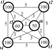
5. Influence of processor heterogeneity—case study. In what follows we want to show that the first difference results in a better load balancing solution than the one provided by the initial algorithm. Let us start from a simple “theoretical” illustration and assume that (as in the above described case of crystal growth modeling) a grid of small volume elements (for which the approximated values of flow are stored) that conforms to the geometry of the flow region is generated. More precisely, a multiblock structured grid of volume elements with 6 blocks with different number of volumes is used (see the example from Figure 3.1.c). Here, inner iterations in each block are associated with a task. Figure 5.1 shows a graph representation of the relationships between those tasks.
Fig. 5.1.Relationships between tasks
The smallest time registered in the system is represented by a time unit in the graph (respectively the communication time between blocks 5 and 6). Computation times registered for the inner iterations performed within each block before an outer iteration (not including any message exchanges) are shown inside graph vertices. The communication overhead generated by sending messages from one block to another is shown along the graph edges. In order to simplify the example we consider that in the solution process there are no delays in message exchanges (the receiver does not wait for incoming messages). To further simplify the example, we consider that the exchange values represent the total combined value of the send and the receive times that take place before an outer iteration.
Let us now consider the case of usingP = 3 processors. When the computing environment is homogeneous, the LTF MFT ACC algorithm distributes tasks as follows:
processor 1: tasks 1, 4 processor 2: tasks 2, 5 processor 3: tasks 3, 6
the longest execution time being the one of processor 1. This time is dominated by the task times: over 200 time units.
When the computing environment is heterogeneous, the first four tasks will be performed resulting in different computing times. We consider the case ofw1= 1.5, w2= 1.8, w3= 1. Thus, processor 3 is the fastest one and processor 2 is the slowest one. The LTF MFT ACC algorithm can provide an initial distribution of the tasks according to a theoretical estimation of the computation time (proportional to the number of volumes inside each block) and the communication time (proportional to the volume of data to be exchanged at block interfaces). In the considered case task distribution suggested by the LTF MFT ACC algorithm will be the same as the above described one, the longest time being still the one of the processor 1: over 300 time units (150 time units for each task).
distribution is the one provided by the initial algorithm. Dividing the registered computation times to calculate relative speedups we will obtain approximately the same values as these registered in the graph described in Figure 5.1. Then the new distribution suggested by the modified algorithm will be:
processor 1: tasks 1, 5 processor 2: tasks 2, 6 processor 3: tasks 3, 4
the longest time being the one of processor 2: over 270 time units (180 time units for the task 2 and 90 time units for task 6), which is an improvement compared to what the initial algorithm resulted in.
In the described case the communication time is not influencing the decision how to distribute tasks. If the ratio of computation time to communication time will be smaller than the above considered one it is possible to have another task distribution. In such a case it is important to also take into account the different speeds of the message exchanges between processors that can be captured by the second proposed modification of the initial algorithm. This case will not be discussed further.
6. Experiment. The proposed modified algorithm was applied to dynamically balance load of the compu-tational effort of the parallel version of the STHAMAS 3D in a heterogeneous computing environment. Detailed test results have been presented in [15]; we mention here the most significant of them.
First, let us provide some background information related to other algorithms mentioned in our paper. The initial LTF MFT ACC algorithm was applied in [6] to a selected CFD problem—a Navier-Stokes simulation of vortex dynamics in the complex wake of a region around hovering rotors. The overset grid system consisted of 857 blocks and approximately 69 million grid points. The experiments running on the 512-processor SGI Origin2000 distributed-shared-memory system showed that the EVAH algorithm performs better than other heuristic algorithms.
Similarly, the CFD test case from the [12] was a solution of a heat transfer problem in a three-dimensional grid consisting of 27-block partitions with 40x40x40 grid points in each block (1.7 millions of grid points). For a range of relative speeds of computers from 1÷1.55 a 21% improvement in the elapsed time was registered.
In our work we have considered a three-dimensional grid applied to the crystal growth simulation escribed above. We used 38-block-partitions with a variable number of grid points: the largest one had 25x25x40 points, while the smallest one had 6x25x13 points (total of 0.3 millions of grid points in the simulation).
We have utilized two computing environments: a homogeneous and a heterogeneous one. The homogeneous computing environment was a Linux cluster of 8 dual PIV Xeon 2GHz Processors with 2Gb RAM and a Myrinet2000 interconnection (http://www.oscer.edu). The heterogeneous computing environment was a Linux network of 17 PCs with variable computational power, from Intel Celeron running at 0.6GHz, with 128Mb RAM to Intel PIV running at 3GHz and with 1Gb RAM (the interval of the relative speeds of computers is 1÷2.9); these machines were connected through an Ethernet 10 Mbs interconnection (http://www.risc.uni-linz.ac.at). Initially block-partitions were distributed uniformly between the processors (e.g. in the case of two pro-cessors, first 19 blocks were send to the first processor, and the remaining 19 blocks were send to the second processor).
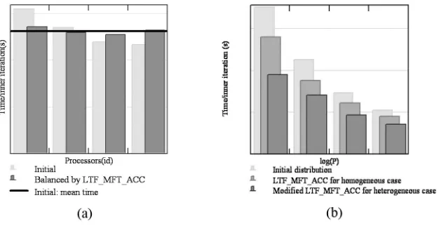
Due to the different number of grid points in individual blocks, the initial algorithm running in the homo-geneous environment recommended a new distribution of nodes. The proposed re-distribution of nodes resulted in a reduction of 17% of the time spent by the code in the inner iteration (Figure 6.1.a).
In the case of the heterogeneous environment, the LTF MFT ACC algorithm performed better: we observed a time reduction ranging from 14% to 20% of the time spent by the CFD code in the inner iteration. A further reduction of the time was obtained when applying the modified LTF MFT ACC algorithm—varying from 20% to 31% (Figure 6.1.b). Comparing time results with these obtained for the initial distribution, a total time reduction attained in our experiments varied from 33% to 45%. We have also found out that the total overhead introduced by the proposed load balancing algorithm was about 6% of the running time.
22 D. Petcu, D. Vizman and M. Paprzycki
Fig. 6.1. Load balancing results : (a) in the case of 4 processors of the homogeneous environment, the LTF MFT ACC
algorithm reduces the differences between the computation time spent by each processor in the inner iteration; (b) in the case of 2, 4, 8 and 16 processors of the heterogeneous environment, theLTF MFT ACCreduces the time per inner iteration, but a further significant reduction is possible using the modifiedLTF MFT ACCalgorithm
Acknowledgments. This work was partially supported by the NanoSim project in the frame of Romanian CEEX Programme.
We would like to thank the Oklahoma University Supercomputing Center and the Research Institute for Symbolic Computing for providing us with access to their computing resources during this study.
REFERENCES
[1] M. Beltran, J.L. Bosque, and A. Guzman,Information policies for load balancing on heterogeneous systems, in Procs. IEEE/ACM Internat. Symp. Cluster Computing and the Grid (2005) pp. 970-976.
[2] J. Cao, D. P. Spooner, S. A. Jarvis, S. Saini, and G. R. Nudd,Agent-based grid load balancing using performance-driven task scheduling, in Procs.IPDPS03, IEEE Computer Press (2003).
[3] S. Chen1, W. Zhang, F. Ma, J. Shen, and M. Li,A novel agent-based load balancing algorithm for Grid computing, in Procs. GCC 2004, H. Jin, Y. Pan, N. Xiao, and J. Sun (Eds.), LNCS 3252 (2004), pp. 156-163.
[4] R.L. Carino and I. Banicescu,A load balancing tool for distributed parallel loops, Cluster Computing, 8 (2005), pp. 313-321. [5] R. David, S. Genaud, A. Giersch, B. Schwarz, and E. Violard,Source code transformations strategies to load-balance
grid applications, in Procs. GRID 2002, M. Parashar (ed.), LNCS 2536, Springer (2002), pp. 82–87.
[6] M. J. Djomehri, R. Biswas, N. Lopez-Benitez,Load balancing strategies for multi-block overset grid applications, NAS-03-007, available athttp://www.nas.nasa.gov/News/Techreports/2003/PDF/nas-03-007.pdf
[7] J. H. Ferziger, M. Peri´c,Computational Methods for Fluid Dynamics, Springer Verlag, Berlin (1996).
[8] H. Gao, A. Schmidt, A. Gupta, P. Luksch,Load balancing for spatial-grid based parallel numerical simulations on clusters of SMPs, in Procs. Euro PDP03, IEEE Computer Press (2003), pp. 75–82.
[9] O. Iliev, M. Sc¨afer,A numerical study of the efficiency ofSIMPLE-type algorithms in computing incompressible flows on streched grids, in Procs. LSSC99, M. Griebel, S. Margenov, P. Yalamov (eds.), Notes on Numerical Fluid Mechanics 73, Vieweg (2000), pp. 207–214.
[10] H.D. Karatza, Job scheduling in heterogeneous distributed systems, Journal of Systems and Software, 56 (2001), pp. 203-212. [11] D. Lukanin, V. Kalaev, A. Zhmakin, Parallel simulation of Czochralski crystal growth, in Procs. PPAM 2003,
R. Wyrzykowski et al, LNCS 3019 (2004), pp. 469–474.
[12] R. U. Payli, E. Yilmaz, A. Ecer, H.U. Akay, and S. Chien, DLBA dynamic load balancing tool for grid computing, in Procs. Parallel CFD04, G. Winter, A. Ecer, F. N. Satofuka, P. Fox (eds.), Elsevier (2005), pp. 391–399
[13] M. Peri´c,A finite volume method for the prediction of three-dimensional fluid flow in complex ducts, Ph.D. Thesis, University of London (1985).
[14] D. Petcu, D. Vizman, J. Friedrich, and M. Popescu, Crystal growth simulation on clusters, in Procs. of HPC2003, I. Banicescu (ed.), Simulation Councils Inc. San Diego (2003), pp. 41–46
[15] D. Petcu, D. Vizman, and M. Paprzycki, Porting CFD codes towards grids—a case study, in Procs. of PPAM 2005, R. Wyrzykowski et al (eds.), LNCS 3911 (2006), in print.
[16] D. Petcu, Adapting a partitioning-based heuristic load-balancing algorithm to heterogeneous computing environments, in Procs. SYNASC 2005, IEEE Computer Society Press, Los Alamitos, pp. 170–173.
[17] P. A. Sackinger, R. A. Brown, J. J. Brown,A finite element method for analysis of fluid flow, heat transfer and free interfaces in Czochralski crystal growth, Internat. J. Numer. Methods in Fluids 9 (1989), pp. 453–492.
[19] D. Sun,A multiblock and multigrid technique for simulations of material processing, Ph.D. Thesis, State University of New York (2001).
[20] C. Z. Xu, F. C. M. Lau,Load Balancing in Parallel Computers: Theory and Practice, Kluwer Academic Publishers, Boston (1996).
[21] S. Yu, J. Casey, and W. Zhou,A load balancing algorithm for Web based server Grids, in Procs. GCC 2003, M. Li et al. (Eds.), LNCS 3033 (2004), pp. 121-128.
Edited by: Przemys law Stipiczy´nski.
Received: May 5, 2006.