The Thirty-Third AAAI Conference on Artificial Intelligence (AAAI-19)
Biomedical Image Segmentation via Representative Annotation
Hao Zheng, Lin Yang, Jianxu Chen,
∗Jun Han, Yizhe Zhang,
Peixian Liang, Zhuo Zhao, Chaoli Wang, Danny Z. Chen
Department of Computer Science and Engineering, University of Notre Dame, Notre Dame, IN 46556, USA
{hzheng3, lyang5, jchen16, jhan5, yzhang29, pliang, zzhao3, cwang11, dchen}@nd.edu
Abstract
Deep learning has been applied successfully to many biomed-ical image segmentation tasks. However, due to the diversity and complexity of biomedical image data, manual annota-tion for training common deep learning models is very time-consuming and labor-intensive, especially because normally only biomedical experts can annotate image data well. Hu-man experts are often involved in a long and iterative process of annotation, as in active learning type annotation schemes. In this paper, we proposerepresentative annotation(RA), a new deep learning framework for reducing annotation effort in biomedical image segmentation. RA uses unsupervised networks for feature extraction and selects representative im-age patches for annotation in the latent space of learned fea-ture descriptors, which implicitly characterizes the underly-ing data while minimizunderly-ing redundancy. A fully convolutional network (FCN) is then trained using the annotated selected image patches for image segmentation. Our RA scheme of-fers three compelling advantages: (1) It leverages the ability of deep neural networks to learn better representations of im-age data; (2) it performs one-shot selection for manual anno-tation and frees annotators from the iterative process of com-mon active learning based annotation schemes; (3) it can be deployed to 3D images with simple extensions. We evaluate our RA approach using three datasets (two 2D and one 3D) and show our framework yields competitive segmentation re-sults comparing with state-of-the-art methods.
Introduction
Image segmentation is a central task in diverse biomedical imaging applications. Recently, deep learning (DL) has been successfully applied to many image segmentation tasks and achieved state-of-the-art or even human-level performance (Ronneberger, Fischer, and Brox 2015; Chen et al. 2016a; 2016b; Zhang et al. 2017; Xu et al. 2017). It is well known that the amount and variety of data that DL networks use for model training drastically affect their performance. How-ever, it is often quite difficult to acquire sufficient training data for DL based biomedical image segmentation tasks, be-cause biomedical image annotation highly depends on ex-pert experience and variations in biomedical data (e.g., dif-ferent modalities and object types) can be large. With limited
∗
J. Chen is now at Allen Institute for Cell Science.
Copyright c2019, Association for the Advancement of Artificial Intelligence (www.aaai.org). All rights reserved.
resources (e.g., money, time, and available experts), reduc-ing annotation efforts while maintainreduc-ing the best possible performance of DL models becomes a critical problem.
Currently, there are two main categories of methods for alleviating the burden of annotation. The methods in the first category aim to utilize unannotated data by leveraging weakly/semi-supervised learning methods (Lin et al. 2016; Yang et al. 2018a; Cheplygina, de Bruijne, and Pluim 2018). Though promising, the performance of such methods is still far from that of supervised learning methods. Accuracy in biomedical analysis is of high importance and thus perfor-mance is a big concern.
The methods in the second category aim to identify and annotate only the most valuable image areas that contribute to the final segmentation accuracy. To achieve this goal, such methods usually explore the following two properties of biomedical images. (1) Biomedical images for a certain type of applications are usuallysimilarto one another (e.g., gland segmentation, heart segmentation). Thus, a great deal of re-dundancy may exist in biomedical image datasets. Fig. 1(a) and (c) show some frequent patterns in glands and heart MR images, respectively. (2) Although regions of interest (ROIs) in biomedical images may have different appearances, we notice that they can be roughly divided into a certain number of groups (e.g., see Fig. 1(b)). Hence, it is helpful to select representative samples to cover the diverse cases in order to achieve good segmentation performance.
sam-(a)
(b) (c)
Figure 1: (a)-(b) Example patches showing similarity and diversity in the gland dataset. The samples in (b) are queried by the active learning (AL) based method (Yang et al. 2017). (c) Similarity in consecutive slices of the 3D heart dataset of HVSMR 2016 (slices#80,#82, . . . ,#88in thexzplane).
ples are annotated. (3) Ineachround of the AL process, the model needs to be applied toallunannotated images, which can take a large amount of time, especially for 3D biomedi-cal images.
To address these issues, in this paper, we propose a new DL framework, representative annotation (RA), to directly select effective instances with high influence and diversity for biomedical image segmentation inone-shot(i.e., no iter-ative process and only training a DL model once). To achieve one-shot selection, we need to address two main challenges. (1) Comparing to AL, in which the model has access to man-ual annotation and can be trained in a supervised manner to extract informative features, the image feature extraction component in our framework has only raw image data and can only be trained in an unsupervised manner. (2) AL meth-ods mainly rely on uncertainty estimation of unannotated images which is not used in our framework. Instead, we need to develop a new criterion for valuable ROIs.
For the first challenge, we investigate and tune various predominant unsupervised models that can be applied to extract image features: autoencoder (AE) (Rumelhart, Hin-ton, and Williams 1986), generative adversarial networks (GANs) (Goodfellow et al. 2014), and variational autoen-coder (VAE) (Kingma and Welling 2013). For the sec-ond challenge, we develop an effective geometry based data selection approach that combines a clustering based method and a max-cover based method. The clustering based method divides the whole dataset intoKclusters and selects the most representative samples from each cluster. To a large extent, it reduces intra-cluster redundancy, but the number of clusters, K, is usually not given. The max-cover based method forms a candidate set containing se-lected samples such that the coverage score for the whole dataset is maximized, which implies that both influential samples from large clusters and diverse samples from differ-ent clusters have a chance to be selected. But, the max-cover problem is NP-hard and the performance of approximation algorithms may degrade a lot when the size of the whole dataset increases. To combine the advantages of both these
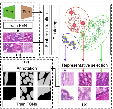
methods, we leverage the clustering based method to reduce intra-cluster redundancy and utilize the max-cover approach to reduce cluster redundancy without sacrificing inter-cluster diversity. In this way, representative (i.e., high influ-ential and diverse) image samples are selected. Fig. 2 out-lines our main idea and steps. Further, our one-shot frame-work enables efficient annotation selection for 3D images.
We conduct extensive experiments, and the results show that our framework outperforms state-of-the-art methods.
Our new RA framework reduces annotation efforts for biomedical image segmentation while maintaining good per-formance. Our main contributions are as follows.
• We decouple representative selection from segmentation, and achieve “one-shot” selection, alleviating the key issue of keeping human experts standby in AL schemes.
• We introduce a clustering-based representative selection method to select representatives for human annotation.
• Our experiments demonstrate that our approach yields higher efficiency and considerably improves the results of state-of-the-art methods on two 2D datasets. Further, we show that our RA framework is effective for a 3D dataset.
Related Work
Dec
Featur
e extraction
Clustering
(a)
(b) Annotation
Train FCNs (c) Train FEN
Representative selection Enc
Figure 2: An overview of our representative annotation (RA) framework: (a) Feature extraction network (FEN) training (Enc: encoder, Dec: decoder); (b) feature extraction and clustering-based representative selection (RS); (c) annota-tion and fully convoluannota-tional network (FCN) training.
the uncertainty of segmentation results, which used consid-erable computational resources. Besides, usingrandom sam-plingto initialize their data selection also makes the initial-ization unstable, which may considerably influence the fi-nal performance. Zhou et al. (Zhou et al. 2018) proposed to find worthy candidates via a combination criterion of the entropy and diversity of patches based on the prediction of CNNs. But, it is not clear how to extend their method from image classification to segmentation. To overcome these drawbacks, we develop a new “one-shot” RA framework that consists of an unsupervised feature extraction network (FEN) and a representative selection (RS) scheme.
Representative Annotation
Our RA framework (see Fig. 2) has three key components: (1) an unsupervised feature extraction network (FEN) that maps each image patch to a low-dimensional feature de-scriptor; (2) a clustering-based algorithm for selecting repre-sentatives from training data; (3) an FCN for segmentation.
Feature Extraction Networks (FENs)
Clustering methods group similar data into a cluster and can be used to reduce intra-cluster redundancy (Aljalbout et al. 2018). In our problem, to map input data to a clustering-friendly feature space, data representation learning is vital. Many unsupervised methods have been proposed for repre-sentation learning. We explore the predominant models (i.e., AE, GAN, and VAE) to design our FEN so that it has good ability for generalization and is fast and stable to train. Autoencoder (AE).AE can be used to learn efficient data
encoding in an unsupervised manner (Rumelhart, Hinton, and Williams 1986). It consists of two networks thatencode an input samplexto a latent representationz anddecode the latent representation back to reconstruct the sample in the original space, as follows:
z∼Enc(x) =qφ(z|x), x˜∼Dec(z) =pθ(x|z). (1)
Training an AE involves finding parameters {θ, φ} that minimize the reconstruction loss,LAE, on the given dataset
X; the objective is given as:
θ∗, φ∗= arg min
θ,φ
LAE(X,(φ◦θ)X). (2)
Generative Adversarial Networks (GANs).GANs (Good-fellow et al. 2014) are explicitly set up to optimize for gener-ative tasks. A GAN consists of a generatorGand a discrim-inatorD (similar structures as a decoder and an encoder of AE, respectively). In training, the generatorG=G(z)∼pg takes a random noise z ∼ pz as input and generates an image. The discriminator D takes an image as input and outputs the probability that the image comes from real data rather than fromG. Ideally, at the end of training,pgcan be shown to matchpdata(i.e.,Gconverges to a good estima-tor ofpdata). The objective function of the min-max game betweenGandDcan be formulated as:
min
G maxD V(D, G) =Ex∼pdata(x)[logD(x)] + Ez∼pz(z)[log(1−D(G(z)))].
(3)
Variational Autoencoder (VAE). Although VAE consists of an encoder and adecoder network, it is quite different from other types of AE models. It makes a strong assump-tion concerning the distribuassump-tion of latent neurons and tries to minimize the difference between a posterior distribution and the distribution of latent neurons with the difference measured by the Kullback-Leibler divergence (Kingma and Welling 2013). Typically, the latent distribution p(z) is a predefined Gaussian distribution, such asz∼ N(0,I). The VAE loss is minus the sum of the expected log likelihood (the reconstruction error) and a prior regularization term:
LV AE =−Eq(z|x)
h
logp(x|z)p(z) q(z|x)
i
=Lpixelllike +Lprior
(4) with
Lpixelllike =−Eq(z|x)[logp(x|z)] (5) and
Lprior=DKL(q(z|x)||p(z)), (6) whereDKLis the Kullback-Leibler divergence.
Hence, we evaluate these methods by the segmentation per-formance. To our best knowledge, we are the first to ex-plore in this direction. We use all these methods as backbone for feature extractors and conduct extensive experiments to compare their potentials (denoted by AE-/GAN-/VAE-FEN below). Our VAE-FEN largely follows the structures in deep convolutional GAN (DCGAN) (Radford, Metz, and Chin-tala 2015). We re-use theencoder anddecoderin the AE-/GAN-based FENs for fair comparison. Experimental results are shown in Table 1.
Representative Selection for 2D Images
Our goal is to select a representative set,Sr, from the whole input unannotated image set,Su, as suggested samples for human annotation. We call this selection process represen-tative selection (RS). Below we will first analyze two intu-itive methods,clustering based RS(denoted byCls-RS) and max-cover based RS(denoted byMC-RS), and then explain why we propose our geometry based selection approach (de-noted byClsMC-RS) that combines the benefits of Cls-RS and MC-RS and addresses their drawbacks.
Cls-RS is a straightforward strategy that utilizes cluster-ing to reduce intra-cluster redundancy. It first conducts clus-tering of the input images and then selects one representa-tive image from each cluster to formSr. A main drawback of this method is that we may need to know the number of clusters,K, beforehand, which is usually unavailable.K di-rectly decides how many images to annotate; thus we should not chooseK arbitrarily. As a result, we may run the risk of over-clustering or under-clustering, and need to deal with unbalanced data. For example, in the gland dataset, normal glands are the majority, and are mainly of a roughly round shape and similar to one another; but, abnormal glands are quite different. Even if we use a large number of clusters, normal glands are still in one cluster while different abnor-mal glands are distinctly separated. Consequently, in the fi-nal candidate set, normal glands become a minority.
MC-RS is another intuitive strategy, inspired by sugges-tive annotation (SA) (Yang et al. 2017). Each image inSu has a representativeness score, and SA aims to find a sub-setSr ⊆ Su such that, for a given budget|Sr| 6 B, the total coverage score|F(Sr, Su)| is maximized. The active learning based SA (Yang et al. 2017) uses uncertainty esti-mation to select a subsetSa ⊂Suas an intermediate step. In our scenario, since we decouple the feature extraction pro-cess from the supervised FCN model, no such uncertainty estimation could be used. Thus, SA degenerates to MC-RS: Each time, among all the unannotated images ofSu, we se-lect the most representativeoneto add toSr such that the coverage score is maximized over the whole set Su. One advantage of this one-by-one selection is that it inherently gives an order list of all unannotated images in which better representative images have higher priorities for manual an-notation. But, MC-RS has two obvious disadvantages. First, the maximum set cover problem is NP-hard and cannot be approximated within1−1
e≈0.632under standard assump-tions (Hochbaum 1997). Our experiments show that, without using uncertainty measures, the performance of the greedy max-cover algorithm is largely jeopardized. Second, MC-RS
Algorithm 1: The Representative Selection Algorithm Input:C={Ci|i= 1, . . . , M}, Ci={Iij|j=
1, . . . , Ni}, δ, r, Sc=∅, Sr=∅;
1 forCiin Cdo
2 Si1=∅,Si2=Ci;
3 while|F(Si1, Ci)|< δ· |Ci|do
4 s∗= arg maxs∈S
i2(F(Si1∪ {s}, Ci)−
F(Si1, Ci));
5 Si1=Si1∪ {s∗},Si2=Si2\ {s∗};
6 Sc =Sc∪Si1;
7 Sa =∅, Sc0 =Sc, N umc=|Sc|;
8 fori= 1, . . . , N umcdo 9 s∗= arg maxs∈S0
c(F(Sa∪ {s}, Sc)−F(Sa, Sc)); 10 Sa =Sa∪ {s∗},Sc0 =Sc0 \ {s∗};
11 L[i][1] =s∗;
12 L[i][2] =P ixelRatio(Sa);
13 fori= 1, . . . , N umcdo
14 ifL[i][2]< r≤L[i+ 1][2]then
15 Sr=Sr∪L[i][1];
16 returnSr
is applied to the whole dataset at once; so it still runs the risk of selecting redundant images from certain groups of large sizes due to unbalanced image patterns.
Hence, based on the above observations and analysis, we propose our two-stageClsMC-RSthat combines clustering based and max-cover based methods. In the first stage, we first conduct agglomerative clustering and use the resulted dendrogram to determine a proper number of clusters, K. Second, we apply the greedy max-cover strategy to select a certain number of images from each cluster to form a tem-poral candidate set,Sc. In this way, (1) we need not knowK
beforehand (Kdirectly decides the finalSr), (2) the whole dataset is divided into multiple clusters of smaller sizes, and max-cover selection works better on smaller sets so that it reduces intra-cluster redundancy while maintaining inter-cluster diversity, and (3) we maintain a balance among dif-ferent clusters, so that scarce samples from small-size clus-ters would not be neglected in the greedy selection. In the second stage, we apply max-cover selection onSc. We select a most representative image fromScone by one to form the finalSr(Sressentially forms an order list). Consequently, (a) since |Sc| < |Su|, the max-cover algorithm works on a smaller set; (b) many images share similar patterns (e.g., nearly round shape glands are common) but could still be divided into several clusters, and this stage helps further re-duce inter-cluster redundancy; (c) since considerable intra-cluster redundancy is reduced in the first stage, the data un-balanced issue is alleviated for the second stage.
Our ClsMC-RS: Clustering + Max-cover. After training FEN, we can make use of it by feeding an image patchI
to theencoder model; the output feature vector,If, of the last fully-connected layer (f c) can be viewed as a high-level representation ofI. In Algorithm 1, we can measure the sim-ilarity between two imagesIiandIjas:
sim(Ii, Ij) =Cosine similarity(Iif, I f
To measure the representativeness of a set Sx of image patches for a patchIof another setSy, we define:
f(Sx, I) = max Ii∈Sx
sim(Ii, I) (8)
It meansIis represented by its most similar patchIiinSx. After patch clustering, each clusterCi (i = 1, . . . , M) contains some number of image patches,Ci = {Iij |j =
1, . . . , Ni}. First, we choose a subset,Si1⊂Ci, which is the most representative forCi. To measure how representative
Si1is forCi, we define the coverage score ofSi1forCias:
F(Si1, Ci) =
X
Ij∈Ci
f(Si1, Ij) (9)
When forming a candidate setSc, it is desired that its over-all coverage score approximates a fraction δof each clus-ter, i.e.,Si1 ⊂Ci,Si1 ⊂ Sc, and|F(Si1, Ci)| ≈δ· |Ci|, whereδcontrols the size ofScand the reduced redundancy in the clusters. Empirically,δis above the “elbow” point in the coverage score curve (i.e., the coverage score increases fast at the beginning and is much flatter at the end).
Having obtained the candidate set Sc, we find a subset
Sr ⊆ Sc = S0c that has the highest coverage score. Itera-tively, we choose one image patch fromSc0 and put it inSr:
I∗= arg max
I∈S0
c
(F(Sr∪ {I}, Sc)−F(Sr, Sc)) (10)
The selection of the patchesI∗essentially sorts the patches inSc based on their representativeness. With more patches selected, the pixel ratio for annotation increases monotoni-cally. We use an arrayLto record the order of the selected patches for annotation and the corresponding pixel ratio.
Finally, experts can label image patches according to the order ofL, until a certain pixel ratior is reached. In our comparative experiments of RA,r= 30%or50%.
Representative Selection for 3D Images
Comparing to 2D image annotation, annotating 3D images is more challenging, partially due to a exponential increase in data volume. Yet, neighboring 2D slices in 3D biomedi-cal image stacks are often quite similar (e.g., see Fig. 1(c)); thus one can potentially exploit this to reduce annotation ef-forts. Intuitively, there are two kinds of selection methods for 3D images:sub-volume basedselection andslice based selection. The former method directly extends our 2D patch-based selection method to 3D datasets. However, this is im-practical due to two issues: (1) 3D FEN is very costly, thus making the size of sub-volumes selected quite small (Wu et al. 2016); (2) human can only label 2D images well. Even if a sub-volume is selected, experts would have to choose a certain plane (e.g.,xy,xz, oryz plane) and label a set of consecutive 2D slices (possibly similar to their neighbors). The latter method, proposed in (C¸ ic¸ek et al. 2016), trains a sparse 3D FCN modelwith some annotated 2D slices. But, a key issue to this method iswhereto annotate. Besides the redundancy among consecutive slices, we also observe that some neighboring slices can vary a lot. Our RA can address these issues. Hence, we propose to directly extend our RA
framework to 3D datasets and select some 2D slices from each orthogonal plane for manual annotation.
Specifically, a 3D image can be analyzed from three or-thogonal directions. By splitting each volume along thexy,
xz, andyzdirections, we obtain three sets of 2D slices. We train three FENs simultaneously on these three sets of 2D slices. For example, given an annotation ratio,ra, our budget of annotating slices in thez-axis isk =bD/rac, whereD is the number of voxels along thez-axis. We can use our 2D RA approach to select the topkrepresentative slices along thez-axis. After obtaining annotation from human experts, we then train a sparse 3D FCN for segmentation.
FCN Models for Supervised Segmentation
2D FCN Model.Since 2D FCNs for biomedical image seg-mentation are well studied, we focus on developing our RA framework for annotation in this paper. To validate the ef-fectiveness of our framework, we adopt the FCN network architecture as in SA (Yang et al. 2017) for fair comparison. Our baseline performance using full annotation matches the corresponding performance given in SA (see Table 1). 3D FCN Model. 3D FCN structure design is more chal-lenging, due to the limits of computing resources that are still not well addressed. Inspired by recent advances on net-work architectures, clique block was proposed in CliqueNet (Yang et al. 2018b). We propose a new 3D FCN model, CliqueVoxNet, for segmentation. First, it uses the stan-dard encoding-decoding FCN diagram to fully incorporate 3D image cues and geometric cues for effective volume-to-volume prediction. Second, it utilizes the state-of-the-art clique block to improve information flow and parameter ef-ficiency, and maintain abundant (both low- and high-level) features for segmenting complicated biomedical structures. Third, it takes advantage of auxiliary side paths for deep supervision (Dou et al. 2016) to improve the gradient flow within the network and stabilize the learning process.
Experiments
To show the effectiveness and efficiency of our RA frame-work, we evaluate RA on two 2D datasets and one 3D dataset: the MICCAI 2015 Gland Segmentation Challenge (GlaS) dataset (Sirinukunwattana et al. 2017), a fungus dataset (Zhang et al. 2017), and the HVSMR 2016 Chal-lenge dataset (Pace et al. 2015). For our representative se-lection (RS), we only need a training set to train our feature extraction network (FEN). Then we train our FCN with an-notated images and evaluate its segmentation on a test set. 2D GlaS Dataset.The GlaS dataset contains 85 training ages (37 benign (BN), 48 malignant (MT)) and 80 test im-ages (33 BN and 27 MT in Part A, 4 BN and 16 MT in Part B). Each image is of size775×522with pixel-wise anno-tation. To train our FEN, we randomly crop patches of size
384×384from the given training set and downsample into
64×64patches, as training data for FEN. Having trained FEN, we crop patches from each training image with a75%
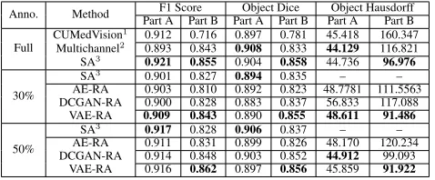
Table 1: Segmentation results on the GlaS dataset.X-RA stands for usingX-based FEN and RS in our RA framework. 1(Chen et al. 2016a);2(Xu et al. 2017);3(Yang et al. 2017).
Anno. Method Part AF1 ScorePart B Part AObject DicePart B Part AObject HausdorffPart B
Full
CUMedVision1 0.912 0.716 0.897 0.781 45.418 160.347
Multichannel2 0.893 0.843 0.908 0.833 44.129 116.821
SA3 0.921 0.855 0.904 0.858 44.736 96.976
30%
SA3 0.901 0.827 0.894 0.835 – –
AE-RA 0.903 0.810 0.892 0.823 48.7781 111.5563
DCGAN-RA 0.900 0.828 0.883 0.837 56.833 117.088
VAE-RA 0.909 0.843 0.890 0.855 48.611 91.486
50%
SA3 0.917 0.828 0.906 0.837 – –
AE-RA 0.911 0.831 0.899 0.826 48.170 120.234
DCGAN-RA 0.914 0.848 0.903 0.852 44.912 99.093
VAE-RA 0.916 0.862 0.897 0.856 45.859 91.922
2D Fungus Dataset.The fungus dataset has 84 fully anno-tated images of size1658×1658. As in (Zhang et al. 2017), we use 4 images as the training set and 80 images as the test set. We randomly crop patches of size450×450from the training set and downsample into 64×64patches to train FEN. We crop patches from each training image with a step size of100pixels and form a set of 784 patches for repre-sentative selection. Results are evaluated using F1 score. 3D HVSMR Dataset.The HVSMR 2016 dataset aims to segment myocardium and great vessel (blood pool) in car-diovascular MR images. 10 3D MR images and their ground truth annotation are provided as training data. The test data, containing another 10 3D MR images, are publicly avail-able; yet their ground truth is kept secret for fair compari-son. The results are evaluated using three criteria: Dice co-efficient, average surface distance (ADB), and symmetric Hausdorff distance. Finally, a scoreS, computed as S = P
class( 1 2Dice−
1 4ADB−
1
30Hausdorff), is used to reflect the overall accuracy of the results and for ranking.
Implementation Details.Our FENs and 2D FCN are imple-mented with PyTorch (Paszke et al. 2017) and Torch7 (Col-lobert, Kavukcuoglu, and Farabet 2011), respectively. An NVIDIA Tesla P100 GPU with 16GB GPU memory is used for both training and testing. The training of FENs and FCN uses similar setups as in (Radford, Metz, and Chintala 2015) and (Yang et al. 2017), respectively. Our 3D CliqueVoxNet is implemented with TensorFlow (Abadi et al. 2016). All the models are initialized using a Gaussian distribution (µ= 0,
σ= 0.01) and trained with the Adam optimization (Kingma and Ba 2015) (β1 = 0.9,β2 = 0.999,=1e-10). We also adopt the “poly” learning rate policy with the power variable equal to 0.9 and the max iteration number equal to 50k. To leverage the limited training data, we perform data augmen-tation (i.e., random roaugmen-tation with 90, 180, and 270 degrees, as well as image flipping along the axial planes) to reduce overfitting.
Main Experimental Results
We first show the state-of-the-art segmentation performance on all the three datasets with full annotation, and then show the effectiveness of our representative annotation (RA) on two aspects: the saved human annotation and the cor-responding segmentation performance compared with the state-of-the-art active learning based method, suggestive
an-Table 2: Segmentation results on the fungus data. VAE∗ =
VAE-FEN + Cls-RS; VAE-RA=VAE-FEN+ClsMC-RS.
Anno. Method Recall Precision F1 Score
Full DAN (Zhang et al. 2017) 0.9020 0.9287 0.9152 Ours (baseline) 0.9118 0.9379 0.9247
30% VAE
∗ 0.9254 0.9211 0.9232
VAE-RA 0.9285 0.9219 0.9252
50% VAE
∗ 0.9268 0.9220 0.9244
VAE-RA 0.9288 0.9226 0.9257
notation (SA) (Yang et al. 2017). Specifically, we measure annotation effort using the number of pixels selected as rep-resentatives by our representative selection (RS) method.
Table 1 gives the segmentation results on the GlaS dataset. First, for fairness of comparison, we use the same FCN model as that in SA and achieve comparable performance as SA withfull annotation. One can see that it attains state-of-the-art performance. Second, using the same FCN structure, we train FCNs with partial annotation with different pixel ra-tios (30%and50%). Table 1 shows that our approach (VAE-RA) achieves competitive or much better results comparing to SA. It is worth noting that, compared to SA with50%of annotated data, our segmentation results are better than SA (∼ 2.5%) on Part B (which contains more malignant sam-ples) while retaining nearly the same performance on Part A. More importantly, our50%VAE-RA closely approaches the performance of full SA on all the three metrics (while there are still some gaps between50%SA and full SA).
Table 2 gives the segmentation results on the fungus dataset. First, our FCN can achieve slightly better perfor-mance than the state-of-the-art methods using full annota-tion. Second, our framework (VAE-RA) can achieve state-of-the-art performance using only30%of the training data, which implies that the fungus dataset is probably less chal-lenging than the gland dataset. Indeed, the fungus dataset contains fewer variations, and its F1 scores on average are higher than those of the GlaS dataset.
Table 3 gives the segmentation results on the 3D heart dataset. First, compared to the state-of-the-art DenseVoxNet, our CliqueVoxNet achieves considerable improvement on all the metrics. Then, we implement sparse 3D FCN models based on CliqueVoxNet. We useuniform annotation (UA) as baseline. Let sk denote the setting of labeling one slice out of every k slices (i.e., the annotation ratio is∼ 1/k). In this dataset, a heart almost occupies the entire stack (see Fig. 1(c)); thus UA is a fairly strong baseline. From Table 3, one can see: (1) With a lower annotation ratio, the overall segmentation performance decreases accordingly (the lower, the faster); (2) the results are not very stable. For example, s10 of UA is slightly better than s2. The reason is that UA cannot ensure that all the slices selected in the setting s10 also belong to s2 (due to the b·c operation for computing slice indices). On the contrary, our RA does not suffer this issue, because inherently it gives an order of slices for an-notation and the slices annotated in sj always belong to si (i < j). As shown in Table 3, overall, our RA achieves much better performance than UA on the same sampling ratios.
Table 3: Segmentation results on the HVSMR 2016 dataset using uniform annotation and representative annotation.
Model Sample
Rate
Myocardium Blood Pool Overall
Score Dice ADB[mm] Hausdorff[mm] Dice ADB[mm] Hausdorff[mm]
DenseVoxNet
Full 0.821 0.964 7.294 0.931 0.938 9.533 -0.161
CliqueVoxNet 0.827 0.924 6.679 0.935 0.797 5.032 0.06
Sparse-CliqueVoxNet
+ Uniform Annotation (UA)
s2 0.792 0.877 5.050 0.926 0.946 7.601 -0.019
s10 0.814 0.826 4.608 0.931 0.961 7.997 0.005
s20 0.791 0.988 6.470 0.934 0.900 6.437 -0.04
s40 0.780 1.334 11.365 0.930 0.942 8.435 -0.374
s80 0.739 1.472 10.227 0.917 1.082 8.932 -0.449
Sparse-CliqueVoxNet
+ Representative Annotation (RA)
s2 0.806 0.928 5.710 0.930 0.871 6.276 0.019
s10 0.812 0.895 5.820 0.928 0.896 6.360 0.016
s20 0.809 0.984 6.874 0.924 0.933 6.470 -0.057
s40 0.786 0.908 4.711 0.916 1.057 8.365 -0.076
s80 0.733 1.250 7.447 0.923 1.010 8.715 -0.276
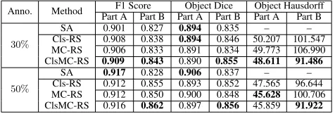
Table 4: Segmentation results on the GlaS dataset using dif-ferent selection schemes.
Anno. Method F1 Score Object Dice Object Hausdorff Part A Part B Part A Part B Part A Part B
30%
SA 0.901 0.827 0.894 0.835 – – Cls-RS 0.908 0.838 0.894 0.846 50.207 101.547 MC-RS 0.906 0.833 0.891 0.834 49.773 106.990 ClsMC-RS 0.909 0.843 0.890 0.855 48.611 91.486
50%
SA 0.917 0.828 0.906 0.837 – –
Cls-RS 0.912 0.855 0.893 0.852 47.565 96.644 MC-RS 0.912 0.850 0.900 0.848 45.628 100.706 ClsMC-RS 0.916 0.862 0.897 0.856 45.859 91.922
datasets demonstrate the effectiveness of our representa-tive annotation framework (X-FEN + ClsMC-RS), which achieves state-of-the-art segmentation performance and saves annotation efforts considerably.
Discussions
On FEN Structures. As shown in Table 1, using features extracted by VAE-based FEN is more beneficial for the sub-sequent representation selection, leading to better segmen-tation results. We think the reasons are: (1) Compared with AE, VAE is a generative model that was originally designed to learn the underlying data distribution and generate new data, while AE learns how to compress data into a con-densed vector with only reconstruction loss; (2) compared with GAN, the output of theencoderin VAE is used to gen-erate a new vector for thedecoderto generate a new image, while the output of the discriminator in GAN is fed to a classifier to differentiate real and fake data. Thus more in-formation could be kept in VAE-extracted features.
On RS Strategies. As shown in Table 4, our ClsMC-RS is better than the other two baselines. First, clustering of image patches reduces intra-cluster redundancy. Inside each clus-ter, we select abundant representatives and the number of patches is controlled by the coverage score (i.e., δ· |Ci|) rather than the size of the cluster. Thus, much redundancy is eliminated. Second, the “max-cover selection” incremen-tally chooses the most representative patches, one by one, which further reduces inter-cluster redundancy without sac-rificing inter-cluster diversity. Hence, the final representative
set for annotation is both influential and diverse. Besides, our ClsMC-RS has two more benefits. (1) Inherently, in the second step, our ClsMC-RS outputs an ordered list, thus en-abling experts to label “better” samples incrementally. (2) After the first step, the size of the candidate setScis largely reduced compared to the whole input set Su (i.e., |Sc| <
|Su|), which could help save more time in the second step. On Time Efficiency. Compared with the state-of-the-art suggestive annotation (SA) (Yang et al. 2017), our RA has better time efficiency. Suppose we need to make annotation suggestion for50%of data. The iterative SA training takes
16 rounds, but our training finishes in one-shot. Each SA round takes∼10minutes to train FCNs; between every two rounds, experts annotate more data based on SA suggestion. More importantly, if we directly apply SA to 3D datasets, the waiting time between two consecutive rounds would in-crease dramatically. With our method, experts do not start annotation until FEN and RS complete, and need not wait for FCN training round after round as in SA. Thus, our training scheme is much more expert-friendly.
Conclusions
In this paper, we presented a new deep learning framework, representative annotation (RA), for reducing annotation ef-fort in biomedical image segmentation. RA combines unsu-pervised feature extraction for representative selection and supervised FCNs for image segmentation. Extensive experi-mental results on three datasets (two 2D and one 3D) show that RA achieves competitive performance as the state-of-the-art suggestive annotation (SA) method (Yang et al. 2017) while using one-shot selection of representatives for annota-tion. Further, RA can be easily extended to 3D datasets and experimental results show great potentials of our method.
Acknowledgments
References
Abadi, M.; Barham, P.; Chen, J.; Chen, Z.; Davis, A.; Dean, J.; Devin, M.; Ghemawat, S.; Irving, G.; Isard, M.; et al. 2016. TensorFlow: A system for large-scale machine learn-ing. InOSDI, volume 16, 265–283.
Aljalbout, E.; Golkov, V.; Siddiqui, Y.; and Cremers, D. 2018. Clustering with deep learning: Taxonomy and new methods. arXiv preprint arXiv:1801.07648.
Chen, H.; Qi, X.; Yu, L.; and Heng, P.-A. 2016a. DCAN: Deep contour-aware networks for accurate gland segmenta-tion. InCVPR, 2487–2496.
Chen, J.; Yang, L.; Zhang, Y.; Alber, M.; and Chen, D. Z. 2016b. Combining fully convolutional and recurrent neural networks for 3D biomedical image segmentation. InNIPS, 3036–3044.
Cheplygina, V.; de Bruijne, M.; and Pluim, J. P. 2018. Not-so-supervised: A survey of semi-supervised, multi-instance, and transfer learning in medical image analysis. arXiv preprint arXiv:1804.06353.
C¸ ic¸ek, ¨O.; Abdulkadir, A.; Lienkamp, S. S.; Brox, T.; and Ronneberger, O. 2016. 3D U-Net: Learning dense volu-metric segmentation from sparse annotation. In MICCAI, 424–432.
Collobert, R.; Kavukcuoglu, K.; and Farabet, C. 2011. Torch7: A matlab-like environment for machine learning. In NIPS Workshop.
Dou, Q.; Chen, H.; Jin, Y.; Yu, L.; Qin, J.; and Heng, P.-A. 2016. 3D deeply supervised network for automatic liver segmentation from CT volumes. InMICCAI, 149–157. Goodfellow, I.; Pouget-Abadie, J.; Mirza, M.; Xu, B.; Warde-Farley, D.; Ozair, S.; Courville, A.; and Bengio, Y. 2014. Generative adversarial nets. InNIPS, 2672–2680. He, K.; Zhang, X.; Ren, S.; and Sun, J. 2016. Deep residual learning for image recognition. InCVPR, 770–778. Hochbaum, D. S. 1997. Approximating covering and pack-ing problems: Set cover, vertex cover, independent set, and related problems. InApproximation Algorithms for NP-hard Problems. Boston, MA, USA: PWS Publishing Co. 94–143. Huang, G.; Liu, Z.; Van Der Maaten, L.; and Weinberger, K. Q. 2017. Densely connected convolutional networks. In CVPR, 4700–4708.
Jain, S. D., and Grauman, K. 2016. Active image segmen-tation propagation. InCVPR, 2864–2873.
J´egou, S.; Drozdzal, M.; Vazquez, D.; Romero, A.; and Ben-gio, Y. 2017. The one hundred layers tiramisu: Fully con-volutional densenets for semantic segmentation. InCVPR Workshop, 1175–1183.
Kingma, D. P., and Ba, J. 2015. Adam: A method for stochastic optimization. InICLR.
Kingma, D. P., and Welling, M. 2013. Auto-encoding vari-ational Bayes.arXiv preprint arXiv:1312.6114.
Li, X.; Chen, H.; Qi, X.; Dou, Q.; Fu, C.-W.; and Heng, P. A. 2017. H-DenseUNet: Hybrid densely connected UNet for liver and liver tumor segmentation from CT volumes. arXiv preprint arXiv:1709.07330.
Lin, D.; Dai, J.; Jia, J.; He, K.; and Sun, J. 2016. Scrib-bleSup: Scribble-supervised convolutional networks for se-mantic segmentation. InCVPR, 3159–3167.
Long, J.; Shelhamer, E.; and Darrell, T. 2015. Fully con-volutional networks for semantic segmentation. InCVPR, 3431–3440.
Pace, D. F.; Dalca, A. V.; Geva, T.; Powell, A. J.; Moghari, M. H.; and Golland, P. 2015. Interactive whole-heart seg-mentation in congenital heart disease. InMICCAI, 80–88. Paszke, A.; Gross, S.; Chintala, S.; Chanan, G.; Yang, E.; DeVito, Z.; Lin, Z.; Desmaison, A.; Antiga, L.; and Lerer, A. 2017. Automatic differentiation in PyTorch. InNIPS Workshop.
Radford, A.; Metz, L.; and Chintala, S. 2015. Unsupervised representation learning with deep convolutional generative adversarial networks. arXiv preprint arXiv:1511.06434. Ronneberger, O.; Fischer, P.; and Brox, T. 2015. U-Net: Convolutional networks for biomedical image segmentation. InMICCAI, 234–241.
Rumelhart, D. E.; Hinton, G. E.; and Williams, R. J. 1986. Learning internal representations by error propagation. In Parallel Distributed Processing: Explorations in the Mi-crostructure of Cognition, 318–362.
Sirinukunwattana, K.; Pluim, J. P. W.; Chen, H.; et al. 2017. Gland segmentation in colon histology images: The GlaS challenge contest. Medical Image Analysis35:489–502. Wu, J.; Zhang, C.; Xue, T.; Freeman, B.; and Tenenbaum, J. 2016. Learning a probabilistic latent space of object shapes via 3D generative-adversarial modeling. InNIPS, 82–90. Xu, Y.; Li, Y.; Wang, Y.; Liu, M.; Fan, Y.; Lai, M.; and Chang, E. I. 2017. Gland instance segmentation using deep multichannel neural networks.IEEE Trans. on Biomed. Eng. 64(12):2901–2912.
Yang, L.; Zhang, Y.; Chen, J.; Zhang, S.; and Chen, D. Z. 2017. Suggestive annotation: A deep active learning frame-work for biomedical image segmentation. InMICCAI, 399– 407.
Yang, L.; Zhang, Y.; Zhao, Z.; Zheng, H.; Liang, P.; Ying, M. T.; Ahuja, A. T.; and Chen, D. Z. 2018a. BoxNet: Deep learning based biomedical image segmentation using boxes only annotation. arXiv preprint arXiv:1806.00593.
Yang, Y.; Zhong, Z.; Shen, T.; and Lin, Z. 2018b. Convo-lutional neural networks with alternately updated clique. In CVPR, 2413–2422.
Yu, L.; Cheng, J.-Z.; Dou, Q.; Yang, X.; Chen, H.; Qin, J.; and Heng, P.-A. 2017. Automatic 3D cardiovascular MR segmentation with densely-connected volumetric ConvNets. InMICCAI, 287–295.
Zhang, Y.; Yang, L.; Chen, J.; Fredericksen, M.; Hughes, D. P.; and Chen, D. Z. 2017. Deep adversarial networks for biomedical image segmentation utilizing unannotated im-ages. InMICCAI, 408–416.