The Thirty-Third AAAI Conference on Artificial Intelligence (AAAI-19)
Data-Adaptive Metric Learning with Scale Alignment
Shuo Chen,
†Chen Gong,
†Jian Yang,
†∗Ying Tai,
‡Le Hui,
†Jun Li
††PCA Lab, Key Lab of Intelligent Perception and System for High-Dimensional Information of Ministry of Education †Jiangsu Key Lab of Image and Video Undersatanding for Social Security
†School of Computer Science and Engineering, Nanjing University of Science and Technology, Nanjing, China ‡Youtu Lab, Tencent
{shuochen, chen.gong, csjyang, le.hui}@njust.edu.cn, [email protected], [email protected]
Abstract
The central problem for most existing metric learning meth-ods is to find a suitable projection matrix on the differences of all pairs of data points. However, a single unified projection matrix can hardly characterize all data similarities accurately as the practical data are usually very complicated, and simply adopting one global projection matrix might ignore impor-tant local patterns hidden in the dataset. To address this issue, this paper proposes a novel method dubbed “Data-Adaptive Metric Learning” (DAML), which constructs a data-adaptive projection matrix for each data pair by selectively combining a set of learned candidate matrices. As a result, every data pair can obtain a specific projection matrix, enabling the proposed DAML to flexibly fit the training data and produce discrimi-native projection results. The model of DAML is formulated as an optimization problem which jointly learns candidate projection matrices and their sparse combination for every data pair. Nevertheless, the over-fitting problem may occur due to the large amount of parameters to be learned. To tackle this issue, we adopt the Total Variation (TV) regularizer to align the scales of data embedding produced by all candidate projection matrices, and thus the generated metrics of these learned candidates are generally comparable. Furthermore, we extend the basic linear DAML model to the kernerlized version (denoted “KDAML”) to handle the non-linear cases, and the Iterative Shrinkage-Thresholding Algorithm (ISTA) is employed to solve the optimization model. Intensive ex-perimental results on various applications including retrieval, classification, and verification clearly demonstrate the superi-ority of our algorithm to other state-of-the-art metric learning methodologies.
Introduction
Metric learning aims to learn a distance function for data pairs to faithfully measure their similarities. It has played an important role in many pattern recognition applica-tions, such as face verification (Liu et al. 2018), person re-identification (Si et al. 2018), and image retrieval (Zhan et al. 2009; Liu, Tsang, and M¨uller 2017).
The well-studied metric learning models are usually global, which means that they directly learn a single
semi-positive definite (SPD) matrixMc =Pb
>
b
P to decide a
Ma-∗
Corresponding author.
Copyright c2019, Association for the Advancement of Artificial Intelligence (www.aaai.org). All rights reserved.
( x, x' )
P::0,P::1,…,P::c w
( x, x' )
Projection Matrix:
(a). Framework of Traditional Metric Learning.
(b). Framework of Our Proposed DAML.
P(w)א ௗൈ
P(w)=P::0+ λ∑k=1wkP::k
Selecting Matrices by using w
Learning w and P::0,P::1,…,P::c Learning Projection Matrix
Combining The Selected Matrices
Projection Distance Result
Distance Result Projection
Pא ௗൈ P࢞ െ P࢞Ԣ
ଶ ଶ
P
P(w)࢞ െP(w)࢞Ԣ ଶଶ
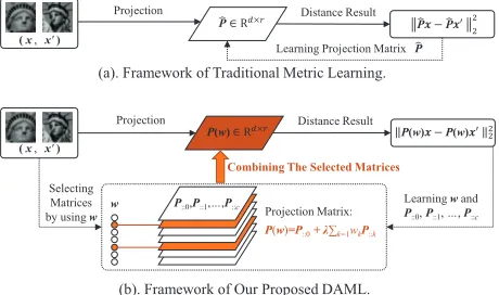
Figure 1: The comparison of traditional metric learning and our proposed model. (a) The traditional method learns a sin-gle global projection matrixPb to distinguish the similarity
of(x,x0). (b) Our proposed DAML jointly learns multiple projection matrices P::0,P::1,· · ·, P::c and their weight vectorw∈Rcfor each data pair(x, x0).
halanobis distance functionD b P(x,x
0) = (x−x0)>
c
M(x−
x0)1 for all data pairs(x,x0)(see Fig. 1(a)), where
b
P can
be understood as a projection matrix. The detailed imple-mentations can be linear projection (Harandi, Salzmann, and Hartley 2017) or non-linear deep neural networks (DNN) (Oh Song et al. 2016). The primitive linear works utilized the supervised information (e.g.must-link and cannot-link) to control the learned distance during their training phases, such as Distance Metric Learning for Clustering (Xing et al. 2003), Large Margin Nearest Neighbor (LMNN) (Wein-berger, Blitzer, and Saul 2006), and Information-Theoretic Metric Learning (ITML) (Davis et al. 2007). To enhance the fitting performance and effectively discover the structure for more complicated data, some recent non-linear methods in-cluding Projection Metric Learning on Grassmann Manifold (Huang et al. 2015) and Geometric Mean Metric Learning (GMML) (Zadeh, Hosseini, and Sra 2016) are proposed to learn the matrices Mc andPb on a manifold instead of the
original linear space. Moreover, by adaptively enriching the
1
For simplicity, the notation of “square” on DPb(x,x 0
training data, Adversarial Metric Learning (Chen et al. 2018; Duan et al. 2018) showed further improvement on the lin-ear metric by discriminating the confusing yet critical data pairs produced by the generator. There are some other methods that replace the linear projectionP xb by the
non-linear formPbW(x)so that the model representation
abil-ity can be boosted, in which the mappingW(·)usually in-dicates a deep neural network. For example, the Convolu-tional Neural Network (CNN) is adopted by Siamese-Net (Zagoruyko and Komodakis 2015) while Multi-Layer Per-ceptron (MLP) is employed by Discriminative Deep Metric Learning (DDML) (Hu, Lu, and Tan 2014). However, the above global metric learning methods are not flexible for handling complex or heterogeneous data, because they all use the same projection operator for all data pairs, which might be inappropriate to characterize the local data prop-erties. As a result, some important patterns carried by the training data are ignored and the learned metric can be inac-curate.
To improve the flexibility of metric learning for fit-ting complex data pairs, various local models were pro-posed from different viewpoints. For example, LMNN was extended to a local version by learning a specific met-ric for each class based on certain classification criterion (Weinberger and Saul 2008). Afterwards, the Instance Spe-cific Distance was proposed to further enhance the met-ric flexibility on each of the training examples (Zhan et al. 2009). Recently, in Parametric Local Metric Learning (Wang, Kalousis, and Woznica 2012), the authors proposed the weighted Mahalanobis distance in which multiple met-ric values are linearly combined. Based on the similar way, the traditional methods LMNN and GMML have also been extended to the local forms by introducing the weighted distances (Bohn´e et al. 2014; Su, King, and Lyu 2017). In contrast to the combination of multiple metrics of PLML, a Gaussian mixture based model (Luo and Huang 2018) par-titioned the metricMc into multiple blocks and proposed a
localized norm to improve the model flexibility. However, these improvements on metricMcare not guaranteed to
con-sistently render reasonable projections for discriminating the similar pairs from dissimilar ones. Therefore, there are also some works aiming at directly refining the projection opera-torPb. For instance, Gated Siamese-Net (Varior, Haloi, and
Wang 2016) employed a gating function to selectively em-phasize the local pattern for the projected data. Similarly, an attention mechanism was utilized in the image matching model (Si et al. 2018), by which the feature-pair alignment can be performed on the projection results.
Although the existing metric learning models have achieved promising results to some extent, most of them cannot adaptively find the suitable projection strategy for different data pairs, as they are not data-adaptive and thus the learning flexibility is rather limited. To this end, we pro-pose a novel metric learning model that generalizes the sin-gle projection matrix to multiple ones, and establish a selec-tive mechanism to adapselec-tively utilize them according to the local property of data points (see Fig. 1(b)). In other words, our method jointly learns multiple candidate matrices and
their sparse combinations for different training pairs. On one hand, every pair of examples is associated with a definite projection matrix which is constructed by wisely selecting and combining a small fraction of candidate matrices. On the other hand, the candidate matrices are also automatically learned to minimize the training loss on each training pair. Considering that such a data-adaptive projection may bring about over-fitting, we further introduce the concept of “met-ric scale” and employ the Total Variation (TV) regularizer to enforce the embedded data produced by different candi-date projection matrices are generally aligned in the same scale. Consequently, the solution space for learning the can-didate projection matrices shrinks and the over-fitting prob-lem caused by scale variations can be effectively alleviated. Thanks to the sparse selections of projection matrices and the operation of scale alignment, every data pair is able to acquire suitable projection to reach discriminative represen-tation for further distance calculations. Therefore, our pro-posed method is termed as “Data-Adaptive Metric Learn-ing” (DAML). The main contributions of this paper are sum-marized below:
• We propose a novel metric learning framework dubbed DAML, which is able to learn adaptive projections for dif-ferent data pairs to enhance the discriminability and flex-ibility of the learned metric.
• A kenerlized version is devised to enable the DAML model to successfully handle the non-linear cases, and an efficient optimization algorithm is designed to solve the proposed model which is guaranteed to converge.
• DAML is empirically validated on various typical datasets and the results suggest that DAML outperforms other state-of-the-art metric learning methodologies.
The Proposed DAML Model
In this section, we first introduce some necessary notations. After that, we establish the basic DAML model in linear space, and then extend it to a kernerlized form to handle the non-linear cases. Finally, we derive the Iterative Shrinkage-Thresholding Algorithm (ISTA) to solve the proposed opti-mization problem.
Notations
Throughout this paper, we write matrices as bold uppercase characters and vectors as bold lowercase characters. Ten-sors are written as Euclid uppercase characters. Let y = (y1, y2,· · ·, yn)> be the label vector of training data pairs X = {(x1,x01),(x2,x02),· · ·,(xn,x0n)}withxi,x0i ∈
Rd, where yi = 1 if xi andx0i are similar, and yi = 0 otherwise. Heredis the data dimensionality andnis the to-tal number of data pairs. GivenP as a three-order tensor, and then thek-th slice of tensorP is written asP::k. The notations|| · ||F,|| · ||1, and|| · ||2 denote the Frobenius-norm, l1-norm, and l2-norm, respectively. The Total Vari-ation (TV) norm ||a||tv for a vector a ∈ Rd is defined
as Pd−1
P::1e1 P::1e2 P::1e3
P::2e1 P::2e3 P
::2e2
(a). ei’sprojection on P::1. (b). ei’sprojection on P::2. (c). Scale Alignment.
P::2e1 P::2e2 P::2e3 P
::1e1 P::1e2 P::1e3
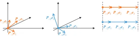
Figure 2: Illustration of scale alignment. The lengths of pro-jectedei(i= 1,2, · · ·, d) by different projection matrices are summed up to the same value. Heredis simply set to 3 for visualization.
Linear DAML Model
Given the matrix Mc ∈ Rd×d in the traditional
Maha-lanobis distance, we know thatMc can be decomposed as
c
M = Pb
>
b
P, and thus the squared Mahalanobis distance
(xi−x0i)>Mc(xi−x0i)betweenxiandx0iis equivalent to the Euclidean distance after their projections byPb,i.e.,
D b
P(xi,x0i) =||P xb i−P xb 0i||22, (1)
wherePb is the projection matrix of the sized×r, andr
is the dimensionality of projection results. Since only one global projection matrixPb is adopted, the traditional
meth-ods are not sufficiently flexible for learning the similarities of all data pairs. To address this limitation, we build a data-adaptive metric learning scheme which automatically gen-erates the suitable projection matrix for each of thendata pairs(xi,x0i) (i = 1,2,· · ·, n). As such, the local prop-erty of dataset can be exploited and an improved metric can be finally learned. To be specific, we propose the following distance regarding tensorP, namely
DP(xi,x0i) =||P(wi)xi−P(wi)x0i|| 2
2, (2) wherePis a three-order tensor stacked by a primitive pro-jection matrixP::0andccandidate matricesP::1,P::2· · ·,
P::c in depth. For thei-th data pair, its specific projection matrix has the form
P(wi) =P::0+λ
Xc
k=1wikP::k, (3) wherewi = (wi1, wi2,· · · , wic)> andwik is the weight of candidate projection matrixP::kfor constructingP(wi). The parameterλ is tuned by the user, andλ = 0 degen-erates our model to the traditional metric learning. From Eq. (3), we see that the data-adaptive projection matrix
P(wi)is decided by the sum of a primitive projection ma-trixP::0and the linear combination of the candidate projec-tion matrices. Therefore, we have to jointly learn the tensor
P ∈ Rr×d×(c+1) for all data pairs as well as the weight vectorwifor thei-th training data pair(xi,x0i).
By taking all n training pairs into consideration and putting allwi into a matrixW = (w1,w2,· · · ,wn), the basic empirical loss for our DAML model is formed as
L(P,W) = 1
n
Xn
i=1l(DP(xi,x 0
i), yi), (4) in which the function l(DP(xi,x0i), yi) evaluates the in-consistency between the labelyi and the model prediction DP(xi,x0i)for the data pair(xi,x0i). Note that practically
not all candidate projection matrices are needed to generate the data-adaptive projection matrixP(wi)for thei-th data pair, so we use the regularizer||W||1to encourage the algo-rithm to sparsely select a small subset of candidate matrices
P::0,P::1,· · ·,P::cto suitably reconstructP(wi). The good news by introducing the combination of can-didate matrices is that the fitting ability of our model can be enhanced. Nevertheless, the bad news is that if we merely minimize the loss function Eq. (4) equipped with the sparse regularizer||W||1 to learn our metric, the over-fitting problem may occur due to the large amount of en-tries in{P::0,P::1,· · · ,P::c}to be learned. Therefore, we should find a way to constrain the final solution to a suitable hypothesis space. Ideally, the linear combination of c+ 1
candidate matrices in {P::0,P::1,· · · ,P::c} can produce exact label for every specific data pair when we minimize l(DP(xi,x0i), yi), which is undesirable and cannot acquire the reasonable general metric. This is because the candidate matrices in{P::0,P::1,· · · ,P::c} can produce the results with arbitrary scales.
To address the over-fitting problem caused by scale variations, we introduce the notation of “metric scale” s(P::k)for P::k (k = 0,1,· · ·, c)and require all scales yielded by {P::0,P::1,· · ·,P::c} to be as close as pos-sible. To this end, we devise the TV regularizer on the scale vector s(P) = (s(P::0), s(P::1),· · · , s(P::c))> ∈
Rc+1, such that the difference between any two of
{s(P::0), s(P::1),· · ·, s(P::c)}can be minimized. Since all projection matrices adopt the comparable scales to measure the distance between pairs of data points, the overfitting caused by scale variations of projection matrices can be ef-fectively alleviated. Specifically, s(P::k) is defined as the sum of squared Mahalanobis distances between the projec-tion on orthonormal bases (i.e.,P::kei) and the origin,i.e.,
s(P::k) =
Xd
i=1DP::k(ei,0) =
Xd
i=1||P::kei−0|| 2 2, (5) whereei is the i-th orthonormal base in Rd. As shown in
Fig. 2, the lengths of projected ei (i = 1,2,· · ·, d) by different projection matrices are summed up to the same value so that the generated scales are perfectly aligned. Since Eq. (5) can be simplified to s(P::k) = ||P::k||2F, the TV regularizer||s(P)||tvcan be easily tackled in the following optimization.
By combining the above empirical loss Eq. (4), sparse regularizer||W||1and TV regularizers(P::k), our DAML model is formally formulated as
min
P,W L(P,W) +α||s(P)||tv+β||W||1, (6)
in which the TV regularizer ||s(P)||tv facilitates the scale alignment and thel1-norm regularizer||W||1performs the sparse selection of candidate projection matrices for data-adaptive projections.
linear regression to predict the weight vectorwz∈Rcfor a
new data pair(z,z0),i.e.,
wz=Q∗(z+z0), (7)
whereQ∗ ∈Rc×dis learned from the linear regression by
minimizing ||QX −W∗||2
F, and X = (x1 +x01,x2+
x02,· · ·,xn +x0n). Based on the predicted weight vector
wz, we know that the distance betweenzandz0equals to
DP∗(z,z0) =||P∗(wz)z−P∗(wz)z0||22, (8)
in whichP∗is learned by solving Eq. (6).
Kernelized DAML Model
In this part, we show that the linear DAML model proposed above can be easily extended to a kernelized form (denoted “KDAML”) to handle the non-linear cases. A symmetric similarity functionκis a kernel (Bishop 2006) if there exists a (possibly implicit) mapping functionφ(·) : X→Hfrom the instance spaceXto a Hilbert spaceHsuch thatκcan be
written as an inner product inH,i.e.,
κ(x,x0) =φ(x)>φ(x0), (9) wherexandx0are examples from the instance spaceX.
To perform the kernel extension, we replace the exam-plesxiandx0iwith their feature mapping resultsφ(xi)and
φ(x0i), and thus the kernelized distanceDκ
P(xi,x0i)which follows Eq. (2) is written as
DκP(xi,x0i) =||P(wi)φ(xi)−P(wi)φ(x0i)|| 2
2, (10) in which the mapping results φ(xi),φ(x0i) ∈ Rh andh is the dimensionality of the Hilbert spaceH. Notice that in
the above kernelized distance, the size of candidate matri-ces P::k (k = 0,1,· · ·, c) are increased tor×hrather than its original size of r ×d. Therefore, it is unrealis-tic to directly learn the parameters in P::k within Rr×h,
because the dimensionality of Hilbert space h is usually assumed to be very high or even infinite (Bishop 2006; Liu and Tsang 2017), which means that the large-scale ma-trixP::kcannot be computed within the limited time. There-fore, according to (Weinberger and Tesauro 2007), we ex-press the candidate matrix P::k as the following form re-garding the mapping resultsφ(i= 1,2,· · ·, n), and obtain
P::k=R::kϕ>, (11)
whereR::k ∈ Rr×n andϕ= (φ(x1),φ(x2),· · ·,φ(xn)) ∈
Rh×n.After that, the problem has been transformed to learn R::0,R::1,· · ·,R::c, of which the sizes are independent with h, and thus the mathematical operations in the original high-dimensional Hilbert space is avoided. By further denoting then-dimensional vectors as
k
i= (κ(xi,x1), κ(xi,x2),· · ·, κ(xi,xn))>,
k0i= (κ(x0i,x1), κ(xi0,x2),· · ·, κ(x0i,xn))>,
(12)
we have DRκ(xi,x0i)
= (φ(xi)−φ(x0i))>(R::0ϕ>+
Xc
k=1R::kϕ >)>
×(R::0ϕ>+
Xc
k=1R::kϕ >)(φ(x
i)−φ(x0i))
= (φ(xi)−φ(x0i))>ϕR(wi)>R(wi)ϕ>(φ(xi)−φ(x0i))
= (ki−k0i) >R(w
i)>R(wi)(ki−k0i), (13)
in which the tensor R ∈ Rr×n×(c+1) is stacked by the
candidate matrices R::0, R::1, · · ·, R::c, and the matrix
R(wi)∈Rr×ncorresponds to the data-adaptive projection
matrixP(wi)in Eq. (2). Compared with the linear DAML model, and additional step required by the kernelized DAML is that the vectorskiandk0iin Eqs. (12) and (13) should be pre-computed for thei-th pair. As long as the kernelκ(·)is specified, we may finally obtain the kernelized distance by Eq. (13). In this paper, we adopt the Gaussian kernel func-tion asκ(·)due to its popularity and computational easiness. Since the distance formulation of KDAML (i.e. Eq. (13)) shares the equivalent mathematical expression with that of linear DAML (i.e.Eq. (2)), it can be directly solved via the same optimization algorithm as the linear DAML. The opti-mization process is detailed in the next section.
Optimization
For algorithm implementation, the loss functionl(Di, yi)in Eq. (4) can be squared loss, squared hinge loss or other pop-ular formulations, which are continuous and have the deriva-tivelD0
i(Di, yi)regardingDi
2. Then we employ the
Itera-tive Shrinkage-Thresholding Algorithm (ISTA) (Rolfs et al. 2012) to solve our problem in Eq. (6). The general ISTA solves a continuous optimization problem with the form
min
θ f(θ) +g(θ), (14)
whereθis the optimization variable,f(θ)is derivable, and g(θ)is usually non-smooth. The solution to Eq. (14) can be found by iteratively optimizing the following function, namely
ΓL(θ,θ(t))
=f(θ(t))+(θ−θ(t))>∇f(θ(t))+L 2||θ−θ
(t)
||22+g(θ),(15)
whereLis Lipschitz constant, and∇f(θ(t))computes the gradient off onθ(t). Eq. (15) admits a unique minimizer, which is
ΠL(θ(t)) = arg min
θ
g(θ)+L 2||θ−(θ
(t) −1
L∇f(θ (t)
))||2 2, (16) whereLis usually manually tuned to satisfy
f(ΠL(θ(t)))+g(ΠL(θ(t)))≤ΓL(ΠL(θ(t)),θ(t)). (17)
To solve our model, we letθ= (P,W), so we havef(θ)
andg(θ)in our model as
f(P,W) =L(P,W) +α||s(P)||tv, (18) and
g(W) =β||W||1. (19)
Then in each iteration, we have to minimize the following
2
Here the notationDP(xi,x0i)is simplified asDifor
function J(P,W)
=β||W||1+
L
2||W−(W
(t)−1
L∇WL(P
(t),W(t)))||2 F
+L
2
P−
P(t)−(1
L(∇PL(P
(t),W(t))+α∇
P||s(P)||tv)
2
F ,
(20)
in which3
(
∇WL(P(t),W(t)) =n1P
n i=1l
0
Di(Di, yi)∇WDi,
∇PL(P(t),W(t)) =n1Pin=1l0Di(Di, yi)∇PDi.
(21)
To minimize above Eq. (20), here we provide the computa-tion results of∇WDiand∇PDirespectively. By using the chain rule of derivate, we can easily obtain that4
(
∇wiDi = 2(A
> 1:i,A
>
2:i,· · ·,A > c:i)>wi, ∇P::kDi= 2
Pc
j=0wikwijxix>i P > ::j.
(22)
Based on above results, the minimizer of Eq. (20) (i.e.the iteration rule) can be summarized as
(
W(t+1)=T
β L
(W(t)−1
L∇WL(P
(t),W(t))),
P(t+1)=P(t)−1
L(∇PL(P
(t),W(t))+α∇
P||s(P)||tv,
(23)
in which the Soft Threshold OperatorTµ(v)(Cai, Cand`es, and Shen 2010) is defined as
Tµ(v) =
v−µ, ifv > µ, v+µ, ifv <−µ,
0, otherwise.
(24)
We summarize the training phase of DAML in Algorithm 1, where Eq. (23) is denoted as
(P(t+1),W(t+1)) =ΠL(P(t),W(t)). (25)
Based on the output of Algorithm 1, the testing steps for a new data pair are described in Algorithm 2. Since KDAML has the equivalent mathematical expression with linear DAML, the training procedure (Algorithm 1) and test-ing steps (Algorithm 2) are directly applicable to KDAML. Finally, we want to explain the convergence of Algorithm 1. Although the traditional ISTA is designed for convex optimization, some extended convergence proofs for non-convex problems have been provided in the prior works such as (Cui 2018). Therefore, the adopted optimization process is theoretically guaranteed to converge to a stationary point.
Experiments
In this section, intensive empirical investigations are con-ducted to validate the effectiveness of our proposed method. In detail, we compare the performance of the DAML and KDAML models with: 1) the classical linear metric learn-ing methods ITML (Davis et al. 2007) and LMNN
(Wein-3∇
P::k||s(P)||tv = 2sign(||P::k||
2
F − ||P::k+1||2F)P::k −
2sign(||P::k||2F − ||P::k−1||2F)P::k. 4
Herewi = (1, λw1, λw2,· · ·, λwc)>andxi =xi−x0i,
respectively. The elementAkjiin the tensorA∈R(c+1)×(c+1)×n equals tox>iP::kP::jxi+x0>i P::kP::jx0i−2x>iP::kP::jx0i.
Algorithm 1Solving Eq. (6) via ISTA.
Input: Training data pairs X = {(xi,x0i)|1 ≤ i ≤ n}; labelsy∈ {0, 1}n; parametersα,β,λ.
Initialize:t= 1;L0= 1;η >1;W(0)=0;P(0)=0.
Repeat:
1). Find the smallest nonnegative integersitsuch that with
b
L=ηitL(t−1)
f(Π
b L(P
(t),W(t))) +g(Π b L(P
(t),W(t)))
≤Γ b L(ΠLb(P
(t)
,W(t)),(P(t),W(t))). 2). SetL(t)=Lband use Eq. (23) to update
(P(t+1),W(t+1)) =ΠL(t)(P(t),W(t)).
3). Updatet=t+ 1.
Until Convergence.
Output:The convergedPandW.
Algorithm 2Distance Computation for New Test Data Pair.
Input: Test data pair(z,z0); the learnd projection tensor
P∗and selection weightsW∗.
Initialize:Regression matrixQ∗= (XX>)−1W∗(X)>.
Procedure:
1). Predict the weights
wz=Q∗(z+z0). 2). Compute the distance
DP∗(z,z0) =||P∗(wz)z−P∗(wz)z0||2
2.
End.
Output:The predicted distanceDP∗(z,z0).
berger, Blitzer, and Saul 2006); 2) the DNN based met-ric learning method DDML (Hu, Lu, and Tan 2014); and 3) state-of-the-art metric learning methods GMDRML (Luo and Huang 2018), LGMML (Su, King, and Lyu 2017), and AML (Chen et al. 2018). All methods are evaluated on retrieval, classification and verification tasks. For the compared methods, we follow the authors’ suggestions to choose the optimal parameters. For the tuning parameters, c is fixed to10 whileα,β andλare all tuned by search-ing the grid {0,0.2,0.4,· · · ,2} to get the best perfor-mances. We follow ITML and use the squared hinge loss as l(DP(xi,x0i), yi)in Eq. (6) for our objective function. The Gaussian kernel function (Bishop 2006) is employed for im-plementing KDAML.
Experiments on Retrieval
Retrieval is one of the most typical applications of metric learning, which aims to search the most similar instances for a query instance (Zhan et al. 2016). In our experiments, we use thePubFigface image dataset (Nair and Hinton 2010) and the Outdoor Scene Recognition (OSR) dataset (Parikh and Grauman 2011) to evaluate the capabilities of all com-pared methods.
individu-Query Top 5 result
(a) Results of 5 nearest neighbors when we query an image on Pubfig dataset. For each queried image, the first row shows the results of LGMML, and the second is the results of our method.
Query Top 5 result
(b) Results of 5 nearest neighbors when we query an image on OSR dataset. For each queried image, the first row shows the results of LGMML, and the second is the results of our method.
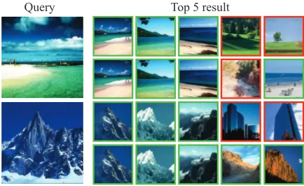
Figure 3: Results of 5 nearest neighbors onPubFigandOSRdatasets for image retrieval. The green box means that the retrieval result is correct, and the red box denotes that the retrieval result is incorrect.
Table 1: The classification error rates (%) of the top 5 retrieval results predicted by all methods on thePubFigandOSRdatasets. The best result in each dataset is in bold. Notation “•” indicates that DAML and KDAML are significantly better than the best baseline method.
Datasets ITML LMNN GMDRML DDML LGMML AML DAML KDAML t-test
PubFig 13.89±0.12 13.65±0.05 13.22±0.34 13.23±0.07 13.15±0.14 13.89±0.11 12.95±0.09 12.89±0.11 •
OSR 24.59±0.11 24.68±0.13 23.51±0.24 23.61±0.17 24.39±0.14 24.32±0.21 23.41±0.12 23.18±0.22 •
als. We follow the experimental setting in (Luo and Huang 2018) and use a512-dimensional Dense Scale Invariant Fea-ture Transform (DSIFT) feaFea-tures (Cheung and Hamarneh 2009) to represent each image. This experiment is run 5 times, where 30 images per person are randomly selected each time as the training data. Fig. 3(a) shows the retrieval results of two queries, and the average classification error rates of top 5 retrieval results are presented in Tab. 1. It can be seen that our proposed DAML and KDAML achieve the lowest error rates,i.e.,12.95%and12.89%, respectively. Moreover, the DNN based method DDML and local method LGMML also yield good performances, but they are still slightly worse than our DAML and KDAML models are re-vealed in Tab. 1.
The second experiment is performed on theOSRdataset. It includes 2688 images from 8 scene categories, which are described by the high-level attribute features (Huo, Nie, and Huang 2016). We also use 30 images for each category as training data, and the other images are used as test data. We repeat this procedure 5 times and use the average error rate to evaluate all methods in Tab. 1. It can be found that our methods DAML and KDAML still obtain the best results
23.41%and23.18%among all comparators. Fig. 3(b) shows the retrieval results of two queries, and it is clear that our method learns a better distance metric than the traditional Mahalanobis distance. Notably, we find that it is quite diffi-cult to distinguish “mountain” and “tall-building” when their images contain blue sky background. Therefore, LGMML fails to consistently return the correct results (see the first row), while our method can still render the satisfactory re-sults. We also perform the t-test (significance level0.05) to validates the superiority of our method to the best baseline.
Experiments on Classification
To evaluate the performances of various compared methods on classification task, we follow the existing work (Ye et al. 2017) and adopt thek-NN classifier (k = 5) based on the learned metrics to investigate the classification error rates of various methods. The datasets are from the well-known UCI repository (Asuncion and Newman 2007), which in-clude MNIST, Autompg, Sonar,Australia, Balance,Isolet,
andLetters. We compare all methods over20 random
tri-als. In each trial,80%of examples are randomly selected as the training examples, and the rest are used for testing. By following the recommendation in (Zadeh, Hosseini, and Sra 2016), the training pairs are generated by randomly pick-ing up1000c(c−1)pairs among the training examples. The average classification error rates of compared methods are showed in Tab. 2, and we find that DAML and KDAML ob-tain the best results. It can be noted that KDAML is gener-ally better than DAML, as the kernel mapping improves the non-linear ability of our model.
Table 2: The classification error rates (%) of all methods on theMNIST, Autompg,Sonar,German-Credit,Balance,Isoletand
Lettersdatasets. The best result in each dataset is in bold. Notation “•” indicates that DAML and KDAML are significantly
better than the best baseline method.
Datasets ITML LMNN GMDRML DDML LGMML AML DAML KDAML t-test
MNIST 14.31±2.32 17.46±5.32 12.21±0.82 11.56±0.07 12.19±0.14 11.52±0.27 11.34±0.12 11.12±0.21 •
Autompg 26.62±3.21 25.92±3.32 24.32±2.71 23.95±1.52 23.56±1.41 25.31±3.22 23.95±5.21 21.45±1.21 •
Sonar 17.02±3.52 16.04±5.31 17.12±5.64 15.31±2.56 21.35±4.01 16.53±3.51 15.64±1.64 15.55±3.65 Australia 17.52±2.13 15.51±2.53 14.12±2.04 15.12±5.23 18.35±1.84 12.95±2.27 13.17±1.97 13.11±2.01 •
Balance 9.31±2.21 9.93±1.62 6.56±2.14 8.12±1.97 7.36±2.14 7.98±2.11 6.21±0.12 6.15±0.17 •
IsoLet 9.23±1.12 3.23±1.23 3.12±0.34 2.68±0.71 3.91±1.14 2.91±2.17 2.98±1.15 2.79±1.32 Letters 6.24±0.23 4.21±2.05 3.54±1.22 5.14±1.04 4.56±2.45 3.22±1.23 3.11±1.05 3.01±1.23 •
0 0.2 0.4 0.6 0.8 1
False Positive Rate (FPR)
0 0.2 0.4 0.6 0.8 1
True Positive Rate (TPR)
(1). PubFig
ITML 0.67897 LMNN 0.72725 GMDRML 0.7532 DDML 0.86222 LGMML 0.87537 AML 0.90116 DAML 0.90746 KDAML 0.9242
0 0.2 0.4 0.6 0.8 1
False Positive Rate (FPR)
0 0.2 0.4 0.6 0.8 1
True Positive Rate (TPR)
(2). LFW
ITML 0.61852 LMNN 0.63748 GMDRML 0.65762 DDML 0.86406 LGMML 0.84448 AML 0.80242 DAML 0.87824 KDAML 0.8911
0 0.2 0.4 0.6 0.8 1
False Positive Rate (FPR)
0 0.2 0.4 0.6 0.8 1
True Positive Rate (TPR)
(3). MVS
ITML 0.56865 LMNN 0.60049 GMDRML 0.6191 DDML 0.65785 LGMML 0.7022 AML 0.71717 DAML 0.75373 KDAML 0.76998
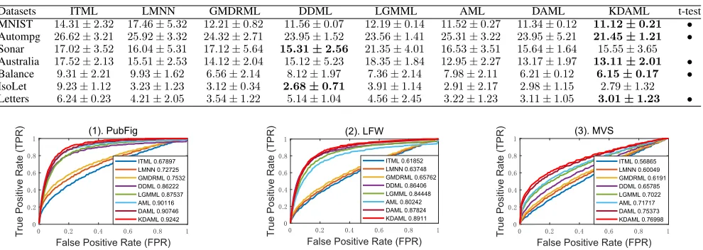
Figure 4: ROC curves of different methods on (a)PubFig, (b)LFW and (c)MVSdatasets. AUC values are presented in the Legends.
Experiments on Verification
We use two face datasets and one image matching dataset to evaluate the capabilities of all compared methods on image verification. For the PubFigface dataset (as described be-fore), the first80%data pairs are selected for training and the rest are used for testing. Similar experiments are performed on theLFWface dataset (Huo, Nie, and Huang 2016) which includes13233unconstrained face images of5749 individ-uals. The image matching dataset MVS(Brown, Hua, and Winder 2011) consists of over 3×10⁴ gray-scale images sampled from 3D reconstructions of the Statue of Liberty (LY), Notre Dame (ND) and Half Dome in Yosemite (YO). By following the settings in (Zagoruyko and Komodakis 2015), LY and ND are put together to form a training set with over105image patch pairs, and104patch pairs in YO are used for testing. The adopted features are extracted by DSIFT (Cheung and Hamarneh 2009) and Siamese-CNN (Zagoruyko and Komodakis 2015) for face datasets (i.e.
PubFigandLFW) and image patch dataset (i.e. MVC),
re-spectively. We plot the Receiver Operator Characteristic (ROC) curve by changing the thresholds of different dis-tance metrics. Then the values of Area Under Curve (AUC) are calculated to quantitatively evaluate the performances of all comparators. From the ROC curves and AUC values in Fig. 4, it is clear to see that DAML and KDAML consis-tently outperform other methods.
Conclusion
In this paper, we propose a metric learning framework named Data-Adaptive Metric Learning (DAML), which generalizes the single global projection matrix of traditional Mahalanobis distance to a local data-adaptive form. The pro-posed projection matrix is combined by a series of weighted candidate matrices for a specific data pair, in which thel1 -norm is employed to sparsely select a small subset of
can-didates to form the suitable combination. Meanwhile, a TV regularizer is utilized to align the produced scales of can-didates so that the over-fitting caused by the arbitrary scale variations can be avoided. Furthermore, we show that such a linear data-adaptive metric can be easily kernelized to han-dle the non-linear cases. The experimental results on various tasks show that the proposed DAML is able to flexibly dis-cover the local data property and acquire more reliable and precise metric than the state-of-the-art metric learning meth-ods. Since the proposed DAML framework is general in na-ture, it is promising to apply DAML to more manifold and DNN based metric learning models for the future works.
Acknowledgments
The authors would like to thank the anonymous review-ers for their critical and constructive comments and sug-gestions. This work was supported by the National Sci-ence Fund (NSF) of China under Grant Nos. U1713208, 61472187 and 61602246, Program for Changjiang Schol-ars, NSF of Jiangsu Province (No: BK20171430), the Fun-damental Research Funds for the Central Universities (No: 30918011319), the “Summit of the Six Top Talents” Pro-gram (No: DZXX-027), the “CAST Lift ProPro-gram for Young Talents”, and the “Outstanding PhD of NJUST” Program (No: AE88902).
References
Asuncion, A., and Newman, D. 2007. Uci machine learning repository.
Bishop, C. M. 2006. Pattern Recognition and Machine
Learning. springer.
Brown, M.; Hua, G.; and Winder, S. 2011. Discriminative learning of local image descriptors. IEEE Transactions on
Pattern Analysis and Machine Intelligence33(1):43–57.
Cai, J.-F.; Cand`es, E. J.; and Shen, Z. 2010. A singular value thresholding algorithm for matrix completion. SIAM
Journal on Optimization20(4):1956–1982.
Chen, S.; Gong, C.; Yang, J.; Li, X.; Wei, Y.; and Li, J. 2018. Adversarial metric learning. InIJCAI, 123–131.
Cheung, W., and Hamarneh, G. 2009. n-sift: n-dimensional scale invariant feature transform. IEEE Transactions on
Im-age Processing18(9):2012–2021.
Cui, A. 2018. Iterative thresholding algorithm based on non-convex method for modified lp-norm regularization mini-mization.arXiv preprint arXiv:1804.09385.
Davis, J. V.; Kulis, B.; Jain, P.; Sra, S.; and Dhillon, I. S. 2007. Information-theoretic metric learning. InICML.
Duan, Y.; Zheng, W.; Lin, X.; Lu, J.; and Zhou, J. 2018. Deep adversarial metric learning. InCVPR, 2780–2789. Harandi, M.; Salzmann, M.; and Hartley, R. 2017. Joint dimensionality reduction and metric learning: A geometric take. InICML, 1943–1950.
Hu, J.; Lu, J.; and Tan, Y.-P. 2014. Discriminative deep metric learning for face verification in the wild. InCVPR. Huang, Z.; Wang, R.; Shan, S.; and Chen, X. 2015. Projec-tion metric learning on grassmann manifold with applicaProjec-tion to video based face recognition. InCVPR, 140–149.
Huo, Z.; Nie, F.; and Huang, H. 2016. Robust and effective metric learning using capped trace norm. InKDD.
Liu, W., and Tsang, I. W. 2017. Making decision trees fea-sible in ultrahigh feature and label dimensions.The Journal
of Machine Learning Research.
Liu, G.; Lin, Z.; Yan, S.; Sun, J.; Yu, Y.; and Ma, Y. 2013. Robust recovery of subspace structures by low-rank repre-sentation. IEEE transactions on pattern analysis and
ma-chine intelligence.
Liu, W.; Xu, D.; Tsang, I.; and Zhang, W. 2018. Metric learning for multi-output tasks. IEEE Transactions on
Pat-tern Analysis and Machine Intelligence.
Liu, W.; Tsang, I. W.; and M¨uller, K.-R. 2017. An easy-to-hard learning paradigm for multiple classes and multiple labels.The Journal of Machine Learning Research.
Luo, L., and Huang, H. 2018. Matrix variate gaussian mix-ture distribution steered robust metric learning. InAAAI.
Nair, V., and Hinton, G. E. 2010. Rectified linear units improve restricted boltzmann machines. InICML, 807–814.
Oh Song, H.; Xiang, Y.; Jegelka, S.; and Savarese, S. 2016. Deep metric learning via lifted structured feature embed-ding. InCVPR, 4004–4012.
Parikh, D., and Grauman, K. 2011. Relative attributes. In
ICCV.
Rolfs, B.; Rajaratnam, B.; Guillot, D.; Wong, I.; and Maleki, A. 2012. Iterative thresholding algorithm for sparse inverse covariance estimation. InNIPS, 1574–1582.
Si, J.; Zhang, H.; Li, C.-G.; Kuen, J.; Kong, X.; Kot, A. C.; and Wang, G. 2018. Dual attention matching net-work for context-aware feature sequence based person re-identification. InCVPR, 132–141.
Su, Y.; King, I.; and Lyu, M. 2017. Learning to rank using localized geometric mean metrics. InSIGIR, 233–241. Varior, R. R.; Haloi, M.; and Wang, G. 2016. Gated siamese convolutional neural network architecture for hu-man re-identification. InECCV, 791–808. Springer. Wang, J.; Kalousis, A.; and Woznica, A. 2012. Parametric local metric learning for nearest neighbor classification. In
NIPS, 1601–1609.
Weinberger, K. Q., and Saul, L. K. 2008. Fast solvers and efficient implementations for distance metric learning. In
ICML, 1160–1167. ACM.
Weinberger, K. Q., and Tesauro, G. 2007. Metric learning for kernel regression. InArtificial Intelligence and Statistics. Weinberger, K. Q.; Blitzer, J.; and Saul, L. K. 2006. Distance metric learning for large margin nearest neighbor classifica-tion. InNIPS, 1473–1480.
Xing, E. P.; Jordan, M. I.; Russell, S. J.; and Ng, A. Y. 2003. Distance metric learning with application to clustering with side-information. InNIPS, 521–528.
Ye, H.-J.; Zhan, D.-C.; Si, X.-M.; and Jiang, Y. 2017. Learn-ing mahalanobis distance metric: ConsiderLearn-ing instance dis-turbance helps. InIJCAI, 866–872.
Zadeh, P.; Hosseini, R.; and Sra, S. 2016. Geometric mean metric learning. InICML, 2464–2471.
Zagoruyko, S., and Komodakis, N. 2015. Learning to com-pare image patches via convolutional neural networks. In
ICCV, 4353–4361.