The Thirty-Third AAAI Conference on Artificial Intelligence (AAAI-19)
Attention-Based Multi-Context Guiding for Few-Shot Semantic Segmentation
Tao Hu,
1,2Pengwan Yang,
2Chiliang Zhang,
3Gang Yu,
4Yadong Mu,
2Cees G. M. Snoek
11University of Amsterdam,2Peking University,3Tsinghua University,4Megvii Inc. (Face++)
[email protected], [email protected], [email protected] [email protected], [email protected], [email protected]
Abstract
Few-shot learning is a nascent research topic, motivated by the fact that traditional deep learning methods require tremen-dous amounts of data. The scarcity of annotated data becomes even more challenging in semantic segmentation since pixel-level annotation in segmentation task is more labor-intensive to acquire. To tackle this issue, we propose an Attention-based Multi-Context Guiding (A-MCG) network, which con-sists of three branches: the support branch, the query branch, the feature fusion branch. A key differentiator of A-MCG is the integration of multi-scale context features between sup-port and query branches, enforcing a better guidance from the support set. In addition, we also adopt a spatial atten-tion along the fusion branch to highlight context informaatten-tion from several scales, enhancing self-supervision in one-shot learning. To address the fusion problem in multi-shot learn-ing, Conv-LSTM is adopted to collaboratively integrate the sequential support features to elevate the final accuracy. Our architecture obtains state-of-the-art on unseen classes in a variant of PASCAL VOC12 dataset and performs favorably against previous work with large gains of 1.1%, 1.4% mea-sured in mIoU in the 1-shot and 5-shot setting.
Introduction
The state-of-the-art in image classification, detection and segmentation have been greatly advanced by convolution neural networks (CNN). Although CNNs exhibit superior performances in a variety of tasks, it has the key problem of being data hungry. Typically gigantic data with annota-tions are required for achieving high accuracy. This issue becomes more severe for pixel-level annotations. In recent years, there emerged a new research thrust which learns new concepts from limited data, known as few-shot learn-ing (Vinyals et al. 2016; Snell, Swersky, and Zemel 2017; Ravi and Larochelle 2017). Though widely explored in tasks like image classification, few-shot learning is rarely consid-ered for dense pixel prediction problems.
Most existing methods in few-shot semantic segmentation are based on the framework shown in the top panel of Fig. 1. Conceptually, the framework is comprised of a support branch and a query branch. The support branch provides dis-criminative support feature to assist the target segmentation,
Copyright c2019, Association for the Advancement of Artificial Intelligence (www.aaai.org). All rights reserved.
Support Branch
Query Branch
Attention based Multi-Context Guiding(A-MCG) Support Image
Query Image
Support Branch
Query Branch Support Image
Query Image Traditional Method
Our Method
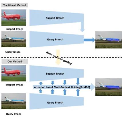
Figure 1: Our motivation. The support image mask is over-laid with ground truth in red, the query image is overover-laid with ground truth in blue. The above is previous method, the below is our method. Our A-MCG network can help the sup-port branch fuse multi-context information to hand on hand guide the query branch.
the query branch is the feature extractor for target segmenta-tion. This paradigm has the following difficulties: (1). Inef-ficient support feature utilization.The feature of the support branch is precious, as it determines the final category the net-work will segment. However, most of the previous methods only consider the single output from the end of the network, which do not take full advantage of the multi-context fea-ture. (2).Lack of attention. As the amount of support and query data is often very small, optimization based on a large amount of data is impossible, some self-supervised methods such as attention should be introduced to make the network concentrate on our target class. (3).Inconvenience in multi-shot learning.The traditional fusion method for multi-shot semantic segmentation is the logical or operation, this inflex-ible approach lacks in exploring the inner common feature between various support images.
Guiding network (A-MCG) shown in the bottom of Fig. 1. Our A-MCG tries to fuse small-to-large scale context infor-mation to globally guide the query branch to make the right segmentation decision. A multi-context feature will largely facilitate the query branch segmentation based on multiple scales of support feature. In addition, we utilize the Resid-ual Attention Module(RAM) (Wang et al. 2017) to carry out a self-supervised attention for further improvement of the segmentation. To deal with multi-shot learning, Conv-LSTM (Xingjian et al. 2015) is incorporated for better fus-ing multi-shot support feature.
Our A-MCG network makes the following contributions: (1). We first propose a Multi-Context Guiding structure to fuse the small-to-large scale context features between sup-port branch and query branch to globally guide the query branch segmentation. (2). We introduce a Residual Attention Module (Wang et al. 2017) in our MCG network to realize the attention mechanism in few-shot learning of segmenta-tion. (3). We embed the Conv-LSTM (Xingjian et al. 2015) module into the end of our network to better merge the fea-ture map from support set in multi-shot semantic segmen-tation. (4). Compared with previous methods, our A-MCG reaches state-of-the-art 61.2%, 62.2% measured in mIoU in the 1-shot and 5-shot setting.
Related Work
Semantic Segmentation. During the early period, the CNN is only employed in the classification tasks, most of them (Krizhevsky, Sutskever, and Hinton 2012; Szegedy et al. 2015) are composed of convolution layers and fully con-nected layers. Fully Convolutional Network(FCN) (Long, Shelhamer, and Darrell 2015) first applies CNN for the task of image semantic segmentation. FCN’s key contribution is building a “fully convolutional” network that takes an input of arbitrary size and produces correspondingly-sized output with efficient inference and learning.
In Deeplab (Chen et al. 2018), Dilated Convolutions are introduced as an alternative to CNN pooling layers in deep part to capture larger context without reducing the image resolution. A module named Atrous Spatial Pyramid Pool-ing (ASPP) is also included in Deeplab where parallel Di-lated Convolution layers with different rates capture multi-scale information. Our method is also illuminated by the context fusion pattern of ASPP and merges the multi-context information by borrowing the multi-scale multi-context from the support branch and the query branch.
Attention Mechanism. In this paper, we mainly talk about two types of attention mechanism: (1). Spatial At-tention such as Residual Attention Module(RAM) (Wang et al. 2017). Inside each Attention Module, an Hourglass-like (Newell, Yang, and Deng ) bottom-up and top-down feedforward structure is used for generating attention map. (2).Channel Attentionlike SENet (Hu, Shen, and Sun 2018). “Squeeze-and-Excitation”(SE) block is designed that adap-tively recalibrates channel-wise feature responses by explic-itly modeling interdependencies between channels. We em-ploy these two types of attention mechanism into our MCG architecture.
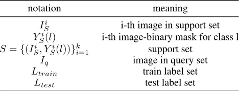
Table 1: Problem Formulation Notations.
notation meaning
ISi i-th image in support set
Yi
S(l) i-th image-binary mask for class l
S={(Ii S, Y
i S(l))}
k
i=1 support set
Iq image in query set
Ltrain train label set
Ltest test label set
Few-Shot Learning in Semantic Segmentation. The first work in few-shot semantic segmentation is OSLSM (Shaban et al. 2017). They proposed the basic paradigm in few-shot segmentation. The support branch and the query branch are constructed by VGG (Simonyan and Zisserman 2014) to supervise training. However, the struc-ture is not fully convolutional, which leads to inefficient utilization of spatial information. Later co-FCN (Rakelly et al. 2018) turns both of the support and query branches into FCN architecture, but the exploration of multi-scale context is not as thorough as our method.
On the other side, OSVOS (Caelles et al. 2017) tries to solve the task of semi-supervised video object segmenta-tion. OSVOS is also based on a fully-convolutional network architecture and transfers generic semantic information to the task of foreground segmentation. OSVOS shows the ef-fectiveness of fine-tuning for video object segmentation, but fine-tuning for every test video is too time-consuming.
Convolutional Long Short-Term Memory.Long Short-Term Memory(LSTM) (Hochreiter and Schmidhuber ) is proposed as a special RNN structure to model long-range dependencies in various previous studies. However, LSTM is not suitable for handling spatiotemporal data because the input-to-state and state-to-state are all full connections thus no spatial information is encoded. To tackle this problem, Conv-LSTM (Xingjian et al. 2015) is put forward by using a convolution operator in the state-to-state and input-to-state transitions.
In our network, Conv-LSTM works as a memory unit to capture and integrate the previous support set feature for better multi-shot learning in semantic segmentation. Conv-LSTM’s advantage is not only modeling the sequential data, but also sequentially filtering and fusing the data by gate mechanism. This method gives us more interpretability and can better smoothen our k-shot learning result compared with traditional fusion method.
Our Method
Problem Formulation
We follow the paradigm and notations in (Shaban et al. 2017), which are detailed in Table 1. The target is to learn a modelf(Iq, S)that, when given a support set S and query
imageIq, predicts a binary maskMˆq for the semantic class
l. The f function is parameterized by neural networks of the support branch and the query branch.
Res3 Res4 Res5 Res1,2
+
C
+
+ +
320x320x3
320x320x3 40x40x512 20x20x1024 20x20x1024
20x20x2048 A1
40x40x512 20x20x1024 20x20x1024
20x20x2048
Support Branch
Query Branch
masking
Res3 Res4 Res5 Res1,2
A2 C C
A1
C
A1
C
A1
C
A1
A2 C A2 C
C A1
C A1
C A1
C
A-MCG(fusion branch)
ConvLSTM C
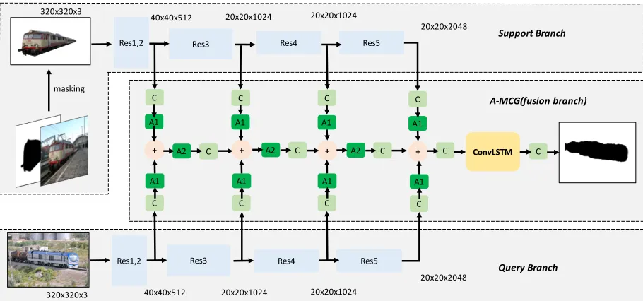
Figure 2: Attention-based Multi-Context Guiding Network Architecture for One-Shot Segmentation. It includes three parts: (1). the support branch. (2). the query branch. (3). A-MCG module. Res1, 2, 3, 4, 5 represent different block in ResNet. C is
1×1convolution unit, stride=2 convolution is employed when the feature map size becomes smaller. We design two exclusive location settings of attention mechanism: A1, A2. The details of the attention architecture are illustrated in Fig. 4.
image-mask pairsD ={(Ij, Yj)}N
j=1whereYj ∈L
H×W train
is the binary mask for training image Ij. At testing, the query images are only annotated for new(unseen) semantic classes i.e. Ltrain ∩Ltest = φ, which leads us to divide
the PASCAL VOC12 dataset like Table 2. This is the key difference between one-shot learning for segmentation and traditional segmentation, what we really care about is the segmentation performance on unseen data. Similar to the ex-tension from one-shot learning to k-shot learning in classifi-cation task, k-shot learning can also be applied in semantic segmentation. In OSLSM (Shaban et al. 2017), k-shot learn-ing results are fused by a logical OR operation between the k binary masks.
Attention Mechanism Review
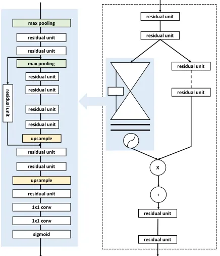
Residual Attention Module(RAM) is first proposed by Wang
et al. (Wang et al. 2017) for image classification. We here review the structure of RAM in Fig. 4. The original RAM proceeds many ablation studies for its setting, we directly use the explored optimal structure. In our paper, we mainly explore the attention location in our MCG module in Sec. Experimental Result.
The RAM actually utilizes a two-scale(down sample 2 times, then up sample 2 times ) Hourglass structure to con-struct a soft attention mask M(x). In the original ResNet (He et al. 2016), residual learning is formulated as:
Hi,c=x+Fi,c(x) (1)
whereFi,c(x)approximates the residual function, i ranges over all spatial positions andc ∈ {1, ..., C}is the index of the channel.
In RAM, the attention module is modified as:
Hi,c= (1 +Mi,c(x))∗Fi,c(x) (2)
M(x) ranges from [0,1] because of the sigmoid function. With M(x) approximating 0, H(x) will approximate original features F(x). The key of RAM lies in M(x), which works as feature selectors that enhance good features and suppress noises from trunk features. This characteristic of RAM is particularly important for few-shot learning cases.
Except that, we also explored the SE block (Hu, Shen, and Sun 2018), which is a typical channel attention struc-ture. Our later ablation study in Sec. Experimental Result shows that SE block fails to compete with RAM under the condition of same parameters.
Attention-based MCG
We propose an Attention-based Multi-Context Guiding net-work (A-MCG) illustrated in Fig. 2. Our A-MCG netnet-work is composed of three parts: (1). the support branch. (2). the query branch. (3). A-MCG(fusion) branch. The backbones of the support branch, the query branch are ResNet101. We elaborate our network as input image size320×320, and their output feature map size is also marked in Fig. 2. No-tably, the convolutions in Res-4, Res-5 blocks are equipped with Dilated Convolution (Chen et al. 2018) whose dilated rate=2. Therefore, the feature map size no long decreases after Res-3, but the receptive field continues to be enlarged due to Dilated Convolution.
ConvLSTM
Conv
Softmax
Output
Unrolling ConvLSTM
Conv
Output
ConvLSTM
Conv
Output
ConvLSTM
Conv
Output 𝟏𝒕𝒉-shot
Q F S Q F S Q F S Q F S
Softmax Softmax Softmax
𝟐𝒕𝒉-shot 𝒌𝒕𝒉-shot
Figure 3: Unrolling view of Conv-LSTM. Q, F, S represents the query branch, the fusion branch, the support branch ac-cordingly. Best viewed in color.
branch segmentation. We attempt two types of attention lo-cation pattern. In the following, we denote thebi
sas feature
maps after Res-i block in the support branch,bi
q as feature
maps after Res-i block in query branch, C as naive convolu-tion(without ReLU (Nair and Hinton 2010), BN), H as our attention function,Fias the mixed features after Res-i block
of the support branch and the query branch.
Therefore, we mainly come up with three variants. (1). Multi-context guiding module:
Fi+1=C{C(bis) +C(b i
q) +Fi} (3)
Multi-context information from both branches are mixed by convolution operation. Notably, convolution here doesn’t in-clude ReLU, BN.
(2). Multi-context guiding with separate attention:
Fi+1=C{H(C(bis)) +H(C(b i
q)) +Fi} (4)
which corresponds to A1 in Fig. 2.
Attention mechanism is employed separately both in the query branch and the support branch.
(3). Multi-context guiding with share attention:
Fi+1=C{H(C(bsi) +C(biq) +Fi)} (5)
which corresponds to A2 in Fig. 2.
Attention mechanism is applied after the fusion of the query branch and the support branch.
Convolutional LSTM for k-shot learning
In previous work, we mainly focus on the circumstance of 1-shot learning in semantic segmentation. How shall we deal with k-shot learning? In OSLSM (Shaban et al. 2017), k-shot learning results are fused by a logical OR operation. How-ever, this straightforward process is unexplainable and fails to utilize the inner relationship between sequential support images.
To better solve this multi-shot learning problem, we at-tempt to embed Conv-LSTM (Xingjian et al. 2015) at the end of the fusion branch as illustrated in Fig. 2. At last, a
1×1 convolution will be appended to generate segmenta-tion probability map.
Conv-LSTM is first applied to the precipitation nowcast-ing task. The key idea of Conv-LSTM is to implement all
residual unit
residual unit max pooling
residual unit
max pooling
residual unit
upsample
residual unit
residual unit
upsample
residual unit
1x1 conv
1x1 conv
sigmoid
residual unit
residual unit
X
+
residual unit
residual unit
re
sidua
l uni
t
residual unit
residual unit
residual unit residual unit
Figure 4: Residual Attention Module(RAM). Left side is an hourglass-like Soft Mask Branch, followed by a sigmoid op-eration. Right side is the whole structure of RAM. “residual unit” is a typical bottleneck structure which is detailed in ResNet (He et al. 2016).
operations, including state-to-state and input-to-state tran-sitions, with kernel-based convolutions. The inner feature of the sequential support image mask can be sustained by Conv-LSTM. We here adopt a popular LSTM variant with “peephole connections” (Gers, Schraudolph, and Schmid-huber 2002). In detail, the three gating functions in Conv-LSTM are calculated according to the equations below:
it=σ(Wx,i⊗Xt+Wh,i⊗Ht−1+Wc,i⊗Ct−1) (6)
ot=σ(Wx,o⊗Xt+Wh,o⊗Ht−1+Wc,o⊗Ct) (7)
ft=σ(Wx,f⊗Xt+Wh,f⊗Ht−1+Wc,f⊗Ct−1) (8)
where we letXt,Htbe the input/hidden state at time t
re-spectively.⊗represents spatio-temporal convolution opera-tor.
Investigating previous H and current X, the recurrent model synthesizes a new proposal for the cell state, namely
˜
Ct=tanh(Wx,c⊗Xt+Wh,c⊗Ht−1) (9) The final cell state is obtained by linearly fusing the new proposalC˜tand previous stateCt−1:
Ct=ftCt−1+itC˜t (10)
wheredenotes the Hadamard product. To continue the recurrent process, it also renders a filtered new H:
In our previous structure, the network is trained on one-shot support set. Once Conv-LSTM is imported into our framework, it will enable us to train with k-shot support set. For every batch(if batch size=1), one query image and k sup-port image masks will be fed into our neural network.
We unroll this procedure in Fig. 3 for better understand-ing the k-shot fusion process. k-shot support image masks enter Conv-LSTM in turn. Conv-LSTM plays a critical role in summarizing the total features of the k-shot support image masks.
For better mixing the feature from the support set in k-shot learning, a function loss is designed as follows:
L=− 1
ks2
k
X
i=0
s
X
m=0,n=0
Ym,nlogXm,n (12)
where Y is binary label, X means the neural network output probability, k is shot number, s represents image size.
This loss enforces our A-MCG module to function well oneverysupport set image rather than only supervises the segmentation of single support image.
Experimental Result
Training details
We implement our code based on the tensorflow frame-work (Abadi et al. 2016). Specially, a scaffold frameframe-work named tensorpack (Wu and others 2016) is used for quickly setting up our experiment. All our models are trained by Stochastic Gradient Descent(SGD) (Bottou 2010) solver with learning rate=1e-4, momentum=0.99 on one Nvidia Ti-tan XP GPU. To fully fill GPU memory, we set the batch size 12. The weights of the support branch and the query branch are initialized with ImageNet (Deng et al. 2009) pre-trained weights. For the weight initialization of A-MCG module, Xavier initialization (Glorot and Bengio 2010) is adopted. All the images in the support and query branch are resized to320×320. No further augmentation is employed except the image resizing. For Batch Normalization(BN) (Ioffe and Szegedy 2015), we employ current batch statistics at training and use the moving average statistics of BN during valida-tion time.
We use the cross-entropy loss as the object function for training the network. The loss is summed up over all the pixels in a mini-batch.
When we experiment with Conv-LSTM for k-shot learn-ing, we set k=5 by default. The max batch size can only be 6 because every time k support image masks will be fed into the support branch. Layer Normalization (Ba, Kiros, and Hinton 2016) is utilized in our Conv-LSTM for speeding up convergence.
Dataset and Metric
Dataset: We utilize dataset PASCAL-5i (Shaban et al.
2017) to conduct our experiment. This dataset is originated from PASCAL VOC12 (Everingham et al. ) and extended annotations from SDS (Hariharan et al. ). The set of 20 classes in PASCAL VOC12 is divided into four sub-datasets as indicated in Table 2. Three sub-datasets are used as the
Table 2: PASCAL-i5group information. The top table dis-plays 4 groups of label and their semantic classes. The bot-tom table shows 4 sub-datasets and their training, validation components.
label set index Semantic Classes
0 aeroplane, bicycle, bird, boat, bottle
1 bus, car, cat, chair, cow
2 diningtable, dog, horse, motorbike, person 3 potted plant, sheep, sofa, train, tv/monitor
sub-dataset train label set val label set
0 1,2,3 0
1 0,2,3 1
2 0,1,3 2
3 0,1,2 3
training label-setLtrain, the left one sub-dataset is utilized
for test label-setLtest.
The training set Dtrain is composed of all image-mask
pairs from PASCAL VOC12 and SDS training sets that in-clude at least one pixel in the segmentation mask from the label-setLtrain. The masks inDtrain are modified into
bi-nary masks by setting pixels whose semantic class are not inLtrain as background classlφ. The test setDtestis from
PASCAL VOC12 and SDS validation sets, and the process-ing procedure for test set Dtest is similar with training set
Dtrain. Our evaluation mIoU is the average of 5 sub-dataset
mIoUs. For a fair comparison with (Shaban et al. 2017), we take the same random seed and sample N=1000 examples for testing each of our models.
Metric:To compare the quantitative performance of the different models, mean intersection over union(mIoU) over two classes is used for our benchmark evaluation. For bi-nary segmentation in our work, we first calculate the 2×
2 confusion matrix, then compute the according IoUl as tpl
tpl+f pl+f nl.tplis the number of true positives for class l, f plis the number of false positives for class l andf nlis the
number of false negatives for class l. The final mIoU is its average over the set of classes.
Ablation Study
Baseline. Our method is mostly compared with
OSLSM (Shaban et al. 2017) and co-FCN (Rakelly et al. 2018). Both of them utilize the VGG (Simonyan and Zisserman 2014) as basic model. Different from them, we adopt ResNet101 (He et al. 2016) as our basic model, for ResNet101 owns much less parameter than VGG16, thus it is less prone to over-fitting. Besides, ResNet also enables larger batch size training in our architecture.
Low High Before After
Before After
Figure 5: Attention Mechanism Visualization. Two images are demonstrated for the comparison between “before atten-tion” and “after attenatten-tion”. The image is overlaid with pre-dicted mask in green. The according histogram of the feature map is displayed in the right side. The feature map’s activa-tion value is normalized to 1. The support image is ignored. Best viewed in color.
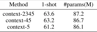
MCG: We explore several factors of our Multi-Context Guiding(MCG) architecture such as (1).fusion width. Fu-sion width is the channel number in the MCG branch, all the features in the support branch and the query branch will be transformed into features with width of fusion width. Differ-ent settings of fusion width are stated in Table 3. (2). multi-context pattern, we try to explore what kind of context com-bination is better for the few-shot learning in Table 4. The number after “context” is the feature we will adopt for fu-sion. For example, context-45 means that only features from Res-4, Res-5 are used for fusion. For convenience, we only proceed the ablation study in the sub-dataset 0 in this part.
From Table 3, we can conclude that when the fusion width is too small such as 64 ,128, the one-shot mIoU is 0.2% lower than width=256. Meanwhile, larger fusion width like 1024 will make the mIoU worse due to over-fitting. Taking into consideration of the balance between mIoU and param-eter cost, we choose fusion width=256 as our default setting. The latter ablation study will also adopt the default value.
As for the multi-context pattern in Table 4, more level context fusion often leads to a better result. Context-2345 outperforms context-5 nearly 2.4% mIoU. This shows that our multi-context guiding strategy works as our motiva-tion. Multi-context information fusion from both the support branch and the query branch could efficiently “support” the query branch’s segmentation.
Table 3: Ablation Study for fusion width. The experiment is conducted on PASCAL-i5 sub-dataset 0.
fusion width 1-shot #params(M)
64 63.4 85.6
128 63.3 86.1
256 63.6 87.2
512 63.6 89.8
1024 63.2 96.1
Table 4: Ablation Study for multi-context pattern. The ex-periment is conducted on PASCAL-i5 sub-dataset 0.
Method 1-shot #params(M)
context-2345 63.6 87.2
context-45 63.2 86.7
context-5 61.2 86.1
Attention Mechanism.We set two variants about the at-tention module: (1). Spatial Attention. Residual Attention Module(RAM) is applied here as a representative method. (2).Channel Attention.SENet (Hu, Shen, and Sun 2018) is explored in our ablation study. At the same time, two at-tention location patterns “separate” and “share” are also ex-plored. “sep” denotes the support branch and query branch adopt separate attention. “share” represents the support branch and query branch share the same attention.
As shown in Table 5. We can find that Spatial Attention works much better than Channel Attention under the circum-stance of same parameters. We conclude that spatial infor-mation is more useful in dense pixel task like image seg-mentation, while channel information plays a more impor-tant role in classification task.
It can be obviously figured out that sharing the same at-tention is basically better than separate atat-tention. We spec-ulate that for the support branch, the input has been already masked so that it does not need attention mechanism, while sharing attention mechanism will make the query branch pay more attention to the support branch’s input mask.
On the other hand, we demonstrate some images’ feature map visualization and feature map histogram in Fig. 5. From the visualization, we can qualitatively observe that the fea-ture map becomes more focusing on the target segmentation objects. As for the feature map histogram, we can quantita-tively discovery that the histogram peak move towards small value. We owe this observation to the fact that the Spatial At-tention enhances good features and suppresses noises from trunk features.
Conv-LSTM for k-shot learning. We mainly contrast two loss variants in Conv-LSTM. (1). 1-loss Conv-LSTM.
single-Table 5: Ablation Study for Attention Mechanism. Chan-nelAttention means SENet Block, SpatialAttention means Residual Attention Block. “sep” denotes the support branch and the query branch adopt separate attention. “share” rep-resents the support branch and the query branch share the same attention.
Method 1-shot #params(M)
MCG 63.3 87.2
MCG-ChannelAttention-sep1 63.6 89.6
MCG-ChannelAttention-share2 61.7 89.8
MCG-SpatialAttention-sep 63.3 93.3
MCG-SpatialAttention-share 65.8 89.5
1
For fair comparison with SpatialAttention method, we change the fusion width to 428 to make #param nearly the same.
2
For fair comparison with SpatialAttention method, we change the fusion width to 480 to make #param nearly the same.
Table 6: Ablation Study for loss function in Conv-LSTM. Baseline is our A-MCG module, we mainly compare the dif-ference between 1-loss Conv-LSTM and 5-loss LSTM. The experiment is conducted on PASCAL-i5 sub-dataset 0.
Method 1-shot 5-shot #params(M)
baseline 65.8 66.2 89.5
1-loss Conv-LSTM 65.1 67.5 90.8
5-loss Conv-LSTM 66.1 67.9 90.8
shot learning. Interestingly, both the 1-shot and 5-shot result on 5-loss LSTM outperform our baseline, which sufficiently validates our motivation.
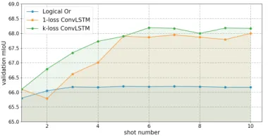
Furthermore, we also conduct k-shot learning where k ranges from 1 to 10 in Fig. 6. k-loss Conv-LSTM fully sur-passes the traditional logical or method in all shot num-ber range. Whenk ≤ 4, the performance of 1-loss Conv-LSTM is less than 5-loss Conv-Conv-LSTM, while partially larger than our baseline. This proves that our 5-loss Conv-LSTM better integrates multi-shot support features than traditional method.
Result in PASCAL VOC.As shown in Table 7, our
A-Table 7: Result on PASCAL-i5 Dataset. All results are computed by taking the average of the 5 sub-datasets in PASCAL-i5. The 5-shot result is obtained by logic or fusion except the method with Conv-LSTM.
Method 1-shot 5-shot #params(M) OSLSM (Shaban et al. 2017) 40.8 43.9 276.7 co-FCN(Multi-class) (Rakelly et al. 2018) 50.9 50.9 –
co-FCN(Overall) (Rakelly et al. 2018) 60.1 60.8 – Baseline 53.0 54.8 85.1
MCG 55.3 56.5 87.2
A-MCG 57.3 57.8 89.5
A-MCG-Conv-LSTM 61.2 62.2 90.8
Figure 6: The relationship between shot number and vali-dation mIoU, we mainly compare among three multi-shot learning fusion strategies: (1). Logical Or. (2). 1-loss Conv-LSTM. (3). k-loss Conv-LSTM(k=5 in our experiment). The experiment is conducted on PASCAL-i5 sub-dataset 0.
Table 8: COCO Dataset result.
method 1-shot 5-shot #params(M)
Baseline 49.98 51.2 85.1
A-MCG-Conv-LSTM 52 54.7 90.8
MCG architecture could outperform nearly 61.2% in 1-shot mIoU, 62.2% in 5-shot mIoU. Based on our baseline, we continue applying the MCG, attention mechanism, Conv-LSTM, reach a new state-of-the-art result on PASCAL-i5
dataset in the end.
Result in COCO Dataset.To evaluate our algorithm in more complex dataset, we evaluate our algorithm in COCO dataset. For the COCO dataset evaluation, we divide the 80 classes into 4 sub-dataset, thus every sub-dataset is com-prised of 20 classes. We cross-validate the performance of our algorithm and the result is shown in Table 8. As COCO dataset owns much more classes compared with Pascal VOC (80 vs 20). The complexity of this dataset makes our per-formance much less obvious in COCO than in PASCAL VOC. However, the result in Table 8 demonstrates that our A-MCG-Conv-LSTM model persistently improve our base-line about 3% mIoU both in 1-shot and 5-shot result.
Conclusion
Acknowledgements
This work is supported by NJUST Key Laboratory of Intel-ligent Perception and Systems for High-Dimensional Infor-mation under Grant No. JYB201701 and Beijing Municipal Commission of Science and Technology under Grant No. 181100008918005.
References
Abadi, M.; Barham, P.; Chen, J.; Chen, Z.; Davis, A.; Dean, J.; Devin, M.; Ghemawat, S.; Irving, G.; Isard, M.; et al. 2016. Tensorflow: A system for large-scale machine learn-ing. InOSDI.
Ba, J. L.; Kiros, J. R.; and Hinton, G. E. 2016. Layer nor-malization.arXiv preprint arXiv:1607.06450.
Bottou, L. 2010. Large-scale machine learning with stochas-tic gradient descent. InProceedings of COMPSTAT’2010.
Caelles, S.; Maninis, K.-K.; Pont-Tuset, J.; Leal-Taix´e, L.; Cremers, D.; and Van Gool, L. 2017. One-shot video object segmentation. InIEEE Conference on Computer Vision and Pattern Recognition.
Chen, L.-C.; Papandreou, G.; Kokkinos, I.; Murphy, K.; and Yuille, A. L. 2018. Deeplab: Semantic image segmentation with deep convolutional nets, atrous convolution, and fully connected crfs. IEEE Transactions on Pattern Analysis and Machine Intelligence.
Deng, J.; Dong, W.; Socher, R.; Li, L.-J.; Li, K.; and Fei-Fei, L. 2009. Imagenet: A large-scale hierarchical image database. InIEEE Conference on Computer Vision and Pat-tern Recognition.
Everingham, M.; Van Gool, L.; Williams, C. K.; Winn, J.; and Zisserman, A. The pascal visual object classes (voc) challenge.International Journal of Computer Vision. Gers, F. A.; Schraudolph, N. N.; and Schmidhuber, J. 2002. Learning precise timing with lstm recurrent networks. Jour-nal of Machine Learning Research.
Glorot, X., and Bengio, Y. 2010. Understanding the diffi-culty of training deep feedforward neural networks. In Inter-national Conference on Artificial Intelligence and Statistics. Hariharan, B.; Arbel´aez, P.; Girshick, R.; and Malik, J. Si-multaneous detection and segmentation. InEuropean Con-ference on Computer Vision.
He, K.; Zhang, X.; Ren, S.; and Sun, J. 2016. Deep resid-ual learning for image recognition. InIEEE Conference on Computer Vision and Pattern Recognition.
Hochreiter, S., and Schmidhuber, J. Long short-term mem-ory.Neural Computation.
Hu, J.; Shen, L.; and Sun, G. 2018. Squeeze-and-excitation networks.IEEE Conference on Computer Vision and Pattern Recognition.
Ioffe, S., and Szegedy, C. 2015. Batch normalization: Accel-erating deep network training by reducing internal covariate shift. InInternational Conference on Machine Learning. Krizhevsky, A.; Sutskever, I.; and Hinton, G. E. 2012. Imagenet classification with deep convolutional neural
net-works. InAdvances in Neural Information Processing Sys-tems.
Long, J.; Shelhamer, E.; and Darrell, T. 2015. Fully convo-lutional networks for semantic segmentation. InIEEE Con-ference on Computer Vision and Pattern Recognition. Nair, V., and Hinton, G. E. 2010. Rectified linear units im-prove restricted boltzmann machines. InInternational Con-ference on Machine Learning.
Newell, A.; Yang, K.; and Deng, J. Stacked hourglass net-works for human pose estimation. InEuropean Conference on Computer Vision.
Rakelly, K.; Shelhamer, E.; Darrell, T.; Efros, A.; and Levine, S. 2018. Conditional networks for few-shot seman-tic segmentation. InInternational Conference on Learning Representations Workshop Papers.
Ravi, S., and Larochelle, H. 2017. Optimization as a model for few-shot learning. InInternational Conference on Learning Representations.
Shaban, A.; Bansal, S.; Liu, Z.; Essa, I.; and Boots, B. 2017. One-shot learning for semantic segmentation. InBritish Ma-chine Vision Conference.
Simonyan, K., and Zisserman, A. 2014. Very deep convolu-tional networks for large-scale image recognition.CoRR. Snell, J.; Swersky, K.; and Zemel, R. 2017. Prototypical networks for few-shot learning. InAdvances in Neural In-formation Processing Systems.
Szegedy, C.; Liu, W.; Jia, Y.; Sermanet, P.; Reed, S.; Anguelov, D.; Erhan, D.; Vanhoucke, V.; Rabinovich, A.; et al. 2015. Going deeper with convolutions. InIEEE Con-ference on Computer Vision and Pattern Recognition. Vinyals, O.; Blundell, C.; Lillicrap, T.; Wierstra, D.; et al. 2016. Matching networks for one shot learning. InAdvances in Neural Information Processing Systems.
Wang, F.; Jiang, M.; Qian, C.; Yang, S.; Li, C.; Zhang, H.; Wang, X.; and Tang, X. 2017. Residual attention network for image classification. InIEEE Conference on Computer Vision and Pattern Recognition.
Wu, Y., et al. 2016. Tensorpack. https://github.com/ tensorpack/.
Xingjian, S.; Chen, Z.; Wang, H.; Yeung, D.-Y.; Wong, W.-K.; and Woo, W.-c. 2015. Convolutional lstm network: A machine learning approach for precipitation nowcasting. In