Using Simulation to Improve Sample-Efficiency of Bayesian
Optimization for Bipedal Robots
Akshara Rai∗∗∗ [email protected]
Robotics Institute, School of Computer Science Carnegie Mellon University, PA, USA
Rika Antonova∗∗∗ [email protected]
Robotics, Perception and Learning, CSC
KTH Royal Institute of Technology, Stockholm, Sweden
Franziska Meier [email protected]
Paul G. Allen School of Computer Science & Engineering University of Washington, Seattle, WA, USA
Christopher G. Atkeson [email protected]
Robotics Institute, School of Computer Science Carnegie Mellon University, PA, USA
∗∗∗These authors contributed equally.
Editor:Bayesian Optimization Special Issue
Abstract
Learning for control can acquire controllers for novel robotic tasks, paving the path for autonomous agents. Such controllers can be expert-designed policies, which typically re-quire tuning of parameters for each task scenario. In this context, Bayesian optimization (BO) has emerged as a promising approach for automatically tuning controllers. However, sample-efficiency can still be an issue for high-dimensional policies on hardware. Here, we develop an approach that utilizes simulation to learn structured feature transforms that map the original parameter space into a domain-informed space. During BO, sim-ilarity between controllers is now calculated in this transformed space. Experiments on the ATRIAS robot hardware and simulation show that our approach succeeds at sample-efficiently learning controllers for multiple robots. Another question arises: What if the simulation significantly differs from hardware? To answer this, we create increasingly ap-proximate simulators and study the effect of increasing simulation-hardware mismatch on the performance of Bayesian optimization. We also compare our approach to other ap-proaches from literature, and find it to be more reliable, especially in cases of high mis-match. Our experiments show that our approach succeeds across different controller types, bipedal robot models and simulator fidelity levels, making it applicable to a wide range of bipedal locomotion problems.
Keywords: Bayesian Optimization, Bipedal Locomotion, Transfer Learning
1. Introduction
Machine learning can provide methods for learning controllers for robotic tasks. Yet, even with recent advances in this field, the problem of automatically designing and learning con-trollers for robots, especially bipedal robots, remains difficult. It is expensive to do learning
c
experiments that require a large number of samples with physical robots. Specifically, legged robots are not robust to falls and failures, and are time-consuming to work with and repair. Furthermore, commonly used cost functions for optimizing controllers are noisy to evaluate, non-convex and non-differentiable. In order to find learning approaches that can be used on real robots, it is thus important to keep these considerations in mind.
Deep reinforcement learning approaches can deal with noise, discontinuities and non-convexity of the objective, but they are not data-efficient. These approaches could take on the order of a million samples to learn locomotion controllers (Peng et al., 2016), which would be infeasible on a real robot. For example, on the ATRIAS robot, 10,000 samples would take 7 days, in theory. But practically, the robot needs to be “reset” between trials and repaired in case of damage. Using structured expert-designed policies can help minimize damage to the robot and make the search for successful controllers feasible. However, the problem is black-box, non-convex and discontinuous. This eliminates approaches like PI2 (Theodorou et al., 2010) which make assumptions about the dynamics of the system and PILCO (Deisenroth and Rasmussen, 2011) which assumes a continuous cost landscape. Evolutionary approaches like CMA-ES (Hansen, 2006) can still be prohibitively expensive, needing thousands of samples (Song and Geyer, 2015).
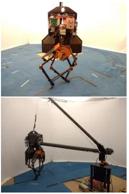
Figure 1: ATRIAS robot. In comparison, Bayesian optimization (BO) is a
sample-efficient optimization technique that is robust to non-convexity and noise. It has been recently used in a range of robotics problems, such as Calandra et al. (2016b), Marco et al. (2017) and Cully et al. (2015). However, sample-efficiency of conventional BO degrades in high dimensions, even for dimensionalities commonly encountered in locomo-tion controllers. Because of this, hardware-only optimiza-tion becomes intractable for flexible controllers and complex robots. One way of addressing this issue is to utilize simula-tion to optimize controller parameters. However, simulasimula-tion- simulation-only optimization is vulnerable to learning policies that ex-ploit the simulation and, because of that, perform well in simulation but poorly on the actual robot. This motivates the development of hybrid approaches that can incorporate simulation-based information into the learning method and then optimize with few samples on hardware.
Towards this goal, our previous work in Antonova, Rai, and Atkeson (2016), Antonova et al. (2017), Rai et al. (2018) presents a framework that uses information from high-fidelity simulators to learn sample-efficiently on hardware. We use simulation to build informed feature transforms that are used to measure controller similarity during BO. Thus, during optimization on hardware, the similarity between controller parameters is informed by how they perform in simulation. With this, it becomes possible to quickly infer which regions of the input space are likely to perform well on hardware. This method has been tested on the ATRIAS biped robot (Figure 1) and shows considerable improvement in sample-efficiency over traditional BO.
robustness of such approaches to simulation-hardware mismatch. We extend our previous work incorporating mismatch estimates (Rai et al., 2018) to this setting. We also conduct extensive comparisons with competitive baselines from prior work, e.g. Cully et al. (2015). The rest of this article is organized as follows: Section 2 provides background for BO, then gives an overview of related work on optimizing locomotion controllers. Section 3.1 de-scribes the idea of incorporating simulation-based transforms into BO; Section 3.2 explains how we handle simulation-hardware mismatch. Sections 4.1-4.5 describe the robot and con-trollers we use for our experiments; Section 4.6 explains the motivation and construction of simulators with various kinds of simulation-hardware mismatch. Section 5 summarizes hardware experiments on the ATRIAS robot. Section 5.2 shows generalization to a different robot model in simulation. Section 5.3 presents empirical analysis of the impact of simulator quality on the performance of the proposed algorithms and alternative approaches.
2. Background and Related Work
This section gives a brief overview of Bayesian optimization (BO), the state-of-the-art re-search on optimizing locomotion controllers, and utilizing simulation information in BO.
2.1. Background on Bayesian Optimization
Bayesian optimization (BO) is a framework for online, black-box, gradient-free global search (Shahriari et al. (2016) and Brochu et al. (2010) provide a comprehensive introduction). The problem of optimizing controllers can be interpreted as finding controller parametersxxx∗that optimize some cost function f(xxx). Here xxx contains parameters of a pre-structured policy; the costf(xxx) is a function of the trajectory induced by controller parametersxxx. For brevity, we will refer to ‘controller parametersxxx’ as ‘controllerxxx’. We use BO to find controllerxxx∗, such that: f(xxx∗) = min
x xx f(xxx).
BO is initialized with a prior that expresses the a priori uncertainty over the value of f(xxx) for each xxx in the domain. Then, at each step of optimization, based on data seen so far, BO optimizes an auxiliary function (calledacquisition function) to select the nextxxxto evaluate. The acquisition function balances exploration vs exploitation. It selects points for which the posterior estimate of the objective f is promising, taking into account both mean and covariance of the posterior. A widely used representation for the cost functionf is a Gaussian process (GP):
f(xxx)∼ GP(µ(xxx), k(xxxi, xxxj))
The prior mean function µ(·) is set to 0 when no domain-specific knowledge is provided. The kernel functionk(·,·) encodes similarity between inputs. If k(xxxi, xxxj) is large for inputs
xxxi, xxxj, thenf(xxxi) strongly influencesf(xxxj). One of the most widely used kernel functions
is the Squared Exponential (SE):
kSE(xxxi, xxxj) =σk2exp − 12(xxxi−xxxj)
Tdiag(```)−2(xxx
i−xxxj)
,
whereσk2, ```are signal variance and a vector of length scales respectively. σk2, ```are referred to as ‘hyperparameters’ in the literature.
well-tuned Mat´ern kernels (Cully et al., 2015). SE and Mat´ern kernels are stationary: k(xxxi, xxxj) depend only on r=xxxi−xxxj ∀xxxi,j. We aim to remove this limitation in a manner
informed by simulation. In future work, incorporating other approaches that relax station-arity (e.g. Martinez-Cantin (2018)) could further improve BO.
2.2. Optimizing Locomotion Controllers
Parametric locomotion controllers can be represented as uuu = πxxx(sss), where π is a policy
structure that depends on parametersxxx. For example,π can be parameterized by feedback gains on the center of mass (CoM), reference joint trajectories, etc. Vectorsss is the state of the robot, such as joint angles and velocities, used in closed-loop controllers. Vector uuu represents the desired control action, for example: torques, angular velocities or positions for each joint on the robot. The sequence of control actions yields a sequence of state transitions, which form the overall ‘trajectory’ [sss0, uuu1, sss1, uuu2, sss2, ...]. This trajectory is used in the cost function to judge the quality of the controllerxxx. In our work, we use structured controllers designed by experts. State of the art research on walking robots featuring such controllers includes Feng et al. (2015) and Kuindersma et al. (2016). The overall optimization then includes manually tuning the parameters xxx. An alternative to manual tuning is to use evolutionary approaches, like CMA-ES, as in Song and Geyer (2015). However, these require a large number of samples and can usually be conducted only in simulation. Optimization in simulation can produce controllers that perform well in simulation, but not on hardware. In comparison, BO is a sample-efficient technique which has become popular for direct optimization on hardware. Recent successes include manipulation (Englert and Toussaint, 2016) and locomotion (Calandra et al., 2016b).
BO for locomotion has been previously explored for several types of mobile robots. These include: snake robots (Tesch et al., 2011), AIBO quadrupeds (Lizotte et al., 2007), and hexapods (Cully et al., 2015). Tesch et al. (2011) optimize a 3-dimensional controller for a snake robot in 10-40 trials (for speeds up to 0.13m/s). Lizotte et al. (2007) use BO to optimize gait parameters for a AIBO robot in 100-150 trials. Cully et al. (2015) learn 36 controller parameters for a hexapod. Even with hardware damage, they can obtain successful controllers for speeds up to 0.4m/s in 12-15 trials.
2.3. Incorporating Simulation Information into Bayesian Optimization
The idea of using simulation to speed up BO on hardware has been explored before. Infor-mation from simulation can be added as a prior to the GP used in BO, such as in Cully et al. (2015). While such methods can be successful, one needs to carefully tune the influence of simulation points over hardware points, especially when simulation is significantly different from hardware.
More generally, approaches such as Kandasamy et al. (2017) and Marco et al. (2017) address trading off computation vs simulation accuracy when selecting the source for the next trial/evaluation (with real world viewed as the most expensive source). Instead, we consider a setting with ample compute resources for simulation, but an extremely small number of experiments on a real robot. This is appropriate for bipedal locomotion with full-scale robots, since these can be expensive to run. Hence, our work does not fall into the ‘multi-fidelity’ BO paradigm, and we instead take a two step approach: pre-computing information needed for kernel transforms in the first stage, then running an ultra-sample efficient version of BO in the second stage on a real robot.
Recently, several approaches proposed incorporating Neural Networks (NNs) into the Gaussian process (GP) kernels (Wilson et al. (2016), Calandra et al. (2016a)). The strength of these approaches is that they can jointly update the GP and the NN. Calandra et al. (2016a) demonstrated how this added flexibility can handle discontinuities in the cost func-tion landscape. However, these approaches do not directly address the problem of incorpo-rating a large amount of data from simulation in hardware BO experiments.
Wilson et al. (2014) explored enhancing GP kernel with trajectories. Their Behavior Based Kernel (BBK) computes an estimate of a symmetric variant of the KL divergence between trajectories induced by two controllers, and uses this as a distance metric in the ker-nel. However, getting an estimate would require samples for each controllerxxxi, xxxj whenever
k(xxxi, xxxj) is needed. This can be impractical, as it involves an evaluation of every controller
considered. To overcome this, the authors suggest combining BBK with a model-based ap-proach. But building an accurate model from hardware data might be an expensive process in itself.
Cully et al. (2015) utilize simulation by defining a behavior metric and collecting best performing points in simulation. This behavior metric then guides BO to quickly find controllers on hardware, and can even compensate for damage to the robot. The search on hardware is conducted in behavior space, and limited to pre-selected “successful” points from simulation. This helps make their search faster and safer on hardware. However, if an optimal point was not pre-selected, BO cannot sample it during optimization.
In our work, we utilize trajectories from simulation to build feature transforms that can be incorporated in the GP kernel used for BO. Our approaches incorporate trajec-tory/behavior information, but ensure that k(xxxi, xxxj) is computed efficiently during BO.
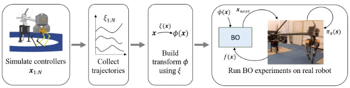
Figure 2: Overview of our proposed approach. Here, πxxx(sss) is the policy (Section 2.2);xxxis a vector
of controller parameters;sssis the state of the robot; ξ(xxx) is a trajectory observed in simulation for xxx;φ(·) is the transform built usingξ(·);f(xxx) is the cost ofxxxevaluated on hardware. BO usesφ(xxx) and evaluated costsf(xxx) to propose next promising controllerxnext.
3. Proposed Approach: Bayesian Optimization with Informed Kernels
In this section, we offer in-depth explanation of approaches from our work in Antonova, Rai, and Atkeson (2016), Antonova et al. (2017), and Rai et al. (2018). This work proposes incorporating domain knowledge into BO with the help of simulation. We evaluate loco-motion controllers in simulation, and collect their induced trajectories, which are then used to build an informed transform. This can be achieved by using a domain-specific feature transform (Section 3.1.1) or by learning to reconstruct short trajectory summaries (Sec-tion 3.1.2). This feature transform is used to construct an informed distance metric for BO, and helps BO discover promising regions faster. Figure 2 gives an overview. In Section 3.2 we discuss how to incorporate simulation-hardware mismatch in to the transform, ensuring that BO can benefit from inaccurate simulations as well.
3.1. Constructing Flexible Kernels using Simulation-based Transforms
High dimensional problems with discontinuous cost functions are very common with legged robots, where slight changes to some parameters can make the robot unstable. Both of these factors can adversely affect BO’s performance, but informed feature transforms can help BO sample high-performing controllers even in such scenarios.
In this section, we demonstrate how to construct such transformsφ(xxx) utilizing simula-tions for a given controllerxxx. We then useφto create an informed kernelkφ(xxxi, xxxj) for BO
on hardware:
tttij=φ(xxxi)−φ(xxxj)
kφ(xxxi, xxxj) =σk2exp
− 12tttTijdiag(```)−2tttij
(1)
3.1.1. The Determinants of Gait Transform
We propose a feature transform for bipedal locomotion derived from physiological features of human walking called Determinants of Gaits (DoG) (Inman et al., 1953). φDoGwas
orig-inally developed for human-like robots and controllers (Antonova, Rai, and Atkeson, 2016), and then generalized to be applicable to a wider range of bipedal locomotion controllers and robot morphologies (Rai et al., 2018). It is based on the features in Table 1.
M1 (Swing leg retraction) – If the maximum ground clearance of the swing foot xf is more than a threshold,M1= 1 (0 otherwise); ensures swing leg retraction.
M2 (Center of mass height) – If CoM heightz stays about the same at the start and end of a step,M2= 1 (0 otherwise); checks that the robot is not falling.
M3(Trunk lean) – If the average trunk leanθis the same at the start and end of a step, M3= 1 (0 otherwise); ensures that the trunk is not changing orientation.
M4 (Average walking speed) – Average forward speed v of a controller per step, M4=vavg;M4 helps distinguish controllers that perform similar onM1−3.
Table 1: Illustration of the features used to construct DoG transform.
φDoG combines features M1−4 per step and scales them by the normalized simulation
time to obtain the DoG score of controllerxxx:
scoreDoG=
tsim
tmax
·
N
X
s=1 4
X
k=1
Mks (2)
Here, subscriptk identifies the feature metric,sis the step number,N is the total number of steps taken in simulation,tsim is time at which simulation terminated (possibly due to a
fall), tmax is total time allotted for simulation. Since larger number of steps lead to higher
DoG, some controllers that chatter (step very fast before falling) could get misleadingly high scores; we scale the scores by tsim
tmax to prevent that. φDoG(xxx) for controller parametersxxxnow
becomes the computed scoreDoG of the resulting trajectories when xxx is simulated. φDoG
essentially aids in (soft) clustering of controllers based on their behaviour in simulation. High scoring controllers are more likely to walk than low scoring ones. Since M1−4 are based on intuitive gait features, they are more likely to transfer between simulation and hardware, as compared to direct cost. The thresholds in M1−3 are chosen according to values observed in nominal human walking from Winter and Yack (1987).
3.1.2. Learning a Feature Transform with a Neural Network
While domain-specific feature transforms can be extremely useful and robust, they might be difficult to generate when a domain expert is not present. This motivates directly learning such feature transforms from trajectory data. In this section we describe our approach to train neural networks to reconstruct trajectory summaries (Antonova et al., 2017) that achieves this goal of minimizing expert involvement.
sim-ulator, we would not have to evaluate each controller on hardware. However, conventional implementations of BO evaluate the kernel function for a large number of points per iter-ation, requiring thousands of simulations each iteration. To avoid this, a Neural Network (NN) can be trained to reconstruct trajectory summaries from a large set of pre-sampled data points. NN provides flexible interpolation, as well as fast evaluation (controller→ tra-jectory summary). Furthermore, trajectories are agnostic to the specific cost used during BO. Thus the data collection can be done offline, and there is no need to re-run simulations in case the definition of the cost is modified.
We use the term ‘trajectory’ in a general sense, referring to several sensory states recorded during a simulation. To create trajectory summaries for the case of locomotion, we include measurements of: walking time (time before falling), energy used during walking, position of the center of mass and angle of the torso. With this, we construct a dataset for NN to fit: a Sobol grid of controller parameters (xxx1:N,N≈0.5 million) along with trajectory
summariesξxxxi from simulation. NN is trained using mean squared loss:
NN input: xxx – a set of controller parameters
NN output: φtrajNN(xxx) = ˆξxxx – reconstructed trajectory summary
NN loss: 12PN
i=1||ξˆxxxi−ξxxxi||
2
The outputs φtrajNN(xxx) are then used in the kernel for BO:
ktrajNN(xxxi, xxxj) =σk2exp −12ttt
T
ijdiag(```)
−2ttt
ij
, tttij =φtrajNN(xxxi)−φtrajNN(xxxj) (3)
Appendix A describes our data collection and training. We did not carefully select the sensory traces used in the trajectory summaries. Instead, we used the most obvious states, aiming for an approach that could be easily adapted to other domains. To apply this approach to a new setting, one could simply include information that is customarily tracked, or used in costs. For example, for a manipulator, the coordinates of the end effector(s) could be recorded at relevant points. Force-torque measurements could be included, if available.
3.2. Kernel Adjustment for Handling Simulation-Hardware Mismatch
Approaches described in previous sections could provide improvement for BO when a high-fidelity simulator is used in kernel construction. In Rai et al. (2018) we presented promising results of experimental evaluation on hardware. However, it is unclear how the performance changes when simulation-hardware mismatch becomes apparent.
In Rai et al. (2018), we also proposed a way to incorporate information about simulation-hardware mismatch into the kernel from the samples evaluated so far. We augment the simulation-based kernel to include this additional information about mismatch, by expand-ing the original kernel by an extra dimension that contains the predicted mismatch for each controllerxxx.
A separate Gaussian process is used to model the mismatch experienced on hardware, starting from an initial prior mismatch of 0: g(xxx)∼ GP(0, kSE(xxxi, xxxj)). For any evaluated
controllerxxxi, we can compute the difference betweenφ(xxxi) in simulation and on hardware:
dxxxi =φ
sim(xxx
i)−φhw(xxxi). We can now use mismatch data {dxxxi|i = 1...n} to construct a
kernelkφwe obtain an adjusted kernel:
φφφxadjxx =
φsim(xxx) ¯ g(xxx)
, tttadjij =φφφxxxadji −φφφxxadjxj
kφadj(xxxi, xxxj) =σ
2
kexp
−1 2(ttt
adj ij )Tdiag
` 1 `1 `1 `2 `2 `2 −2
tttadjij
(4)
The similarity between pointsxxxi, xxxj is now dictated by two components: representation in
φ space and expected mismatch. This construction has an intuitive explanation: Suppose controllerxxxiii results in walking when simulated, but falls during hardware evaluation. kφadj
would register a high mismatch for xxxi. Controllers would be deemed similar toxxxi only if
they have both similar simulation-basedφ(·) and similar estimated mismatch. Points with similar simulation-based φ(·) and low predicted mismatch would still be ‘far away’ from the failedxxxi. This would help BO sample points that still have high chances of walking in
simulation, but are in a different region of the original parameter space. In the next section, we present a more mathematically rigorous interpretation for kφadj.
3.2.1. Interpretation of Kernel with Mismatch Modeling
Let us consider a controllerxxxi evaluated on hardware. The difference between
simulation-based and hardware-simulation-based feature transform forxxxi is dxxxi =φ
sim(xxx
i)−φhw(xxxi). The ‘true’
hardware feature transform for xxxiii is φhw(xxxiii) = φsim(xxxiii) −dxxxiii. After n evaluations on
hardware,{dxxxi|i= 1...n}can serve as data for modeling simulation-hardware mismatch. In
principle, any data-efficient modelg(·) can be used, such as GP (a multi-output GP in case φ(·) > 1D). With this, we can obtain an adjusted transform: ˆφhw(xxx) = φsim(xxx)−g¯(xxx), where ¯g(·) is the output of the model fitted using{dxxxi|i= 1, ...n}.
Supposexxxnewhas not been evaluated on hardware. We can use ˆφhw(xxxnew) =φsim(xxxnew)−
¯
g(xxxnew) as the adjusted estimate of what the output of φ should be, taking into account
what we have learned so far about simulation-hardware mismatch.
Let’s construct kernelkv2
φadj(xxxi, xxxj) that uses these hardware-adjusted estimates directly:
qqqadjij = ˆφhw(xxxi)−φˆhw(xxxj)
= (φsim(xxxi)−¯g(xxxi))−(φsim(xxxj)−¯g(xxxj))
= (φsim(xxxi)−φsim(xxxj))
| {z }
v v vφ
−(¯g(xxxi)−¯g(xxxj))
| {z }
vvvg
kv2
φadj(xxxi, xxxj) =σ
2
kv0 exp
−12(qqqadjij )T diag(```)−2qqqadjij
=σ2exp−1 2
(vvvφ−vvvg)T diag(```)−2(vvvφ−vvvg)
=σ2exp−12
v
vvTφdiag(```)−2vvvφ+vvvTg diag(```)
−2vvv
g−prodij
whereprodij = 2vvvTφdiag(```)−2vvvg
Using exp(a+b+c) = exp(c)·exp(a+b), we have:
kv2
φadj(xxxi, xxxj) =σ
2exp(prod
ij) exp
−1 2 v v
vTφdiag(```)−2vvvφ+vvvTg diag(```)−2vvvg
Which can be written as:
kv2
φadj(xxxi, xxxj) =σ
2exp(prod
ij) exp
−12(tttadjij )T diag
```
```
−2
tttadjij
tttadjij =
v vvφ
vvvg
=
φsim(xxxi)−φsim(xxxj)
¯
g(xxxi)−¯g(xxxj)
Compare this tokφadj from Equation 4:
kφadj(xxxi, xxxj) =σ
2
kexp
−1 2(ttt
adj ij ) Tdiag `1 `1 `1 `2 `2 `2 −2
tttadjij (5)
Now we see thatkv2
φadj andkφadj have a similar form. Hyperparameters`1``1, `21 ``22 provide
flexibil-ity inkφadj as compared to having only vector```ink
v2
φadj. They can be adjusted manually or
with Automatic Relevance Determination. Forkv2
φadj, the role of signal variance is captured
byσ2exp(−prodij). This makes the kernel nonstationary in the transformedφspace. Since
kφadj is already non-stationary inxxx, it is unclear whether non-stationarity of k
v2
φadj in the
transformed φspace has any advantages.
The above discussion shows that kφadj proposed in Rai et al. (2018) is motivated both
intuitively and mathematically. It aims to use a transform that accounts for the hardware mismatch, without adding extra non-stationarity in the transformed space. While the above analysis shows the connection betweenkφadj andk
v2
φadj, a more systematic empirical analysis
would be beneficial as part of future work.
4. Robots, Simulators and Controllers Used
In this section we give a concise description of the robots, controllers and simulators used in experiments with BO for bipedal locomotion. Our approach is applicable to a wide range of bipedal robots and controllers, including state-of-the-art controllers (Feng et al., 2015). We work with two different types of controllers – a reactively stepping controller and a human-inspired neuromuscular controller (NMC). The reactively stepping controller is model-based: it uses inverse-dynamics models of the robot to compute desired motor torques. In contrast, NMC is model-free: it computes desired torques using hand-designed policies, created with biped locomotion dynamics in mind. These controllers exemplify two different and widely used ways of controlling bipedal robots. In addition to this, we show results on two different robot morphologies – a parallel bipedal robot ATRIAS, and a serial 7-link biped model. Our hardware experiments are conducted on ATRIAS; the 7-link biped is only used in simulation. Our success on both robots shows that the approaches developed in this paper are widely applicable to a range of bipedal robots and controllers.
4.1. ATRIAS Robot
4.2. Planar 7-link Biped
The second robot used in our experiments is a 7-link biped (Thatte and Geyer, 2016). It has a trunk and segmented legs with ankles, with actuators in the hip, knees and ankles. The inertial properties of its links are similar to an average human (Winter and Yack, 1987). This 7-link model is a canonical simulator for testing bipedal walking algorithms, for example in Song and Geyer (2015). It is a simplified two-dimensional simulator for a large range of humanoid robots, like Atlas (Feng et al., 2015). We use this simulator to study the generalizability of our proposed approaches to systems different from ATRIAS.
4.3. Feedback Based Reactive Stepping Policy
We design a parametric controller for controlling the CoM height, torso angle and the swing leg by commanding desired ground reaction forces and swing foot landing location.
Fx=Kpt(θdes−θ)−Kdtθ˙ Fz =Kpz(zdes−z)−Kdzz˙ xp =k(v−vtgt) +Cd+ 0.5vT
Here, Fx is the desired horizontal ground reaction force (GRF), Kpt and Kdt are the
proportional and derivative feedback gains on the torso angle θ and velocity ˙θ. Fz is the
desired vertical GRF, Kpz and Kdz are the proportional and derivative gains on the CoM
heightzand vertical velocity ˙z. zdes andθdes are the desired CoM height and torso lean. xp
is the desired foot landing location for the end of swing; v is the horizontal CoM velocity, kis the feedback gain that regulatesv towards the target velocityvtgt. C is a constant and
dis the distance between the stance leg and the CoM;T is the swing time.
The desired GRFs are sent to ATRIAS inverse dynamics model that generates desired motor torquesτf, τb. Details can be found in Rai et al. (2018). This controller assumes no
double-support, and the swing leg takes off as soon as stance is detected. This leads to a highly dynamic gait, posing a challenging optimization problem.
To investigate the effects of increasing dimensionality on our optimization, we construct two controllers with different number of free parameters:
• 5-dimensional controller : optimizing 5 parameters [Kpt, Kdt, k, C, T]
(zdes,θdes and the feedback on zare hand tuned)
• 9-dimensional controller : optimizing all 9 parameters of the high-level policy [Kpt, Kdt, θdes, Kpz, Kdz, zdes, k, C, T]
4.4. 16-dimensional Neuromuscular Controller
We use neuromuscular model policies, as introduced in Geyer and Herr (2010), as our controller for the 7-link planar human-like biped model. These policies use approximate models of muscle dynamics and human-inspired reflex pathways to generate joint torques, producing gaits that are similar to human walking.
Though originally developed for explaining human neural control pathways, this con-troller has recently been applied to prosthetics and bipeds, for example Thatte and Geyer (2016) and Van der Noot et al. (2015). This controller is capable of generating a variety of locomotion behaviours for a humanoid model – walking on rough ground, turning, run-ning, and walking upstairs, making it a very versatile controller (Song and Geyer, 2015). This is a model-free controller as compared to the reactive-stepping controller, which was model-based.
4.5. 50-dimensional Virtual Neuromuscular Controller
Another model-free controller we use on ATRIAS is a modified version of Batts et al. (2015). VNMC maps a neuromuscular model, similar to the one described in Section 4.4 to the ATRIAS robot’s topology and emulates it to generate desired motor torques. We adapt VNMC by removing some biological components while preserving its basic functionalities. The final version of the controller consists of 50 parameters including low-level control parameters, such as feedback gains, as well as high level parameters, such as desired step length and desired torso lean. Details can be found in Rai et al. (2018). When optimized using CMA-ES, it can control ATRIAS to walk on rough terrains with height changes of
±20 cm in planar simulation (Batts et al., 2015).
4.6. Increasingly Inaccurate Simulators
To compare the performance of different methods that can be used to transfer information from simulation to hardware, we create a series of increasingly approximate simulators. These simulators emulate increasing mismatch between simulation and hardware and its ef-fect on the information transfer. In this setting, the high-fidelity ATRIAS simulator (Martin et al., 2015), which was used in all the previous simulation experiments becomes the “hard-ware”. Next we make dynamics approximations to the original simulator, which are used commonly in simulators to decrease fidelity and increase simulation speed. For example, the complex dynamics of harmonic drives are approximated as a torque multiplication, and the boom is removed from the simulation, leading to a two-dimensional simulator. These approximate simulators now become the“simulators”. As the approximations in these sim-ulators are increased, we expect the performance of methods that utilize simulation for optimization on hardware to deteriorate.
The details of the approximate simulators are described in the two paragraphs below: 1. Simulation with simplified gear dynamics : We replace the original high-fidelity gear model with a commonly used approximation for geared systems – multiplying the rotor torque by the gear ratio. This reduces the simulation time to about a third of the original simulator, but leads to an approximate gear dynamics model.
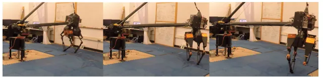
Figure 3: ATRIAS during BO with DoG-based kernel (video: https://youtu.be/hpXNFREgaRA)
The advantage of such an arrangement is that we can test the effect of un-modelled and wrongly modelled dynamics on information transfer between simulation and hardware. Even in our high-fidelity original simulator, there are several un-modelled components of the actual hardware. For example, the non-rigidness of the robot parts, misaligned motors and relative play between joints. In our experiments, we find that the 50-dimensional VNMC is a sensitive controller, with little hope of directly transferring from simulation to hardware. Anticipating this, we can now test several methods of compensating for this mismatch using our increasingly approximate simulators.
5. Experiments
We will now present our experiments on optimizing controllers that are 5, 9, 16 and 50 dimensional. We split our experiments into three categories: hardware experiments on the ATRIAS robot, simulation experiments on the 7-link biped and experiments using simulators with different levels of mismatch. We demonstrate that our proposed approach is able to generalize to different controllers and robot structures and is also robust to simulation inaccuracies. The sections below present experimental results, while Appendix A gives further details on data collection, BO implementation and kernel generation.
5.1. Hardware Experiments on the ATRIAS Robot
In this section we describe experiments conducted on the ATRIAS robot (hardware from Section 4.1). These experiments were conducted around a boom. The cost function used in our experiments is a slight modification of the cost used in Song and Geyer (2015):
cost=
(
100−xf all,if fall
||vavg−vtgt||,if walk
(6)
wherexf allis distance covered before falling,vavg is average speed per step andvtgtcontains
target velocity profile, which can be variable. This cost function heavily penalizes falls, and encourages walking controllers to track target velocity.
We do multiple runs of each algorithm on the robot. Each run typically consists of 10 experiments on the robot. All BO runs start from scratch, with an uninformed GP prior. At the end of the run, the GP posterior has 10 data points, depending on the experiment. Each robot trial is designed to be between 30s to 60s long and the robot is reset to its “home” position between trials.
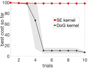
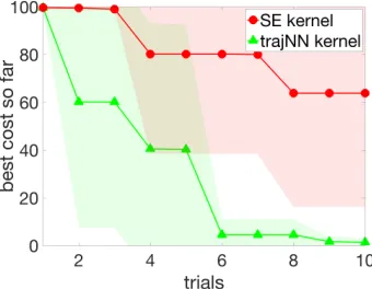
(a) BO for 5D controller. BO with SE finds walking points in 4/5 runs within 20 trials. BO with DoG-based kernel finds walking points in 5/5 runs within 3 trials.
(b) BO for 9D controller. BO with SE doesn’t find walking points in 3 runs. BO with DoG-based kernel finds walking points in 3/3 runs within 5 trials.
Figure 4: BO for 5D and 9D controller on ATRIAS robot hardware. Plots show mean best cost so far. Shaded region shows±one standard deviation. From Rai et al. (2018).
(first reported in Rai et al. (2018)). The second set describes a new set of experiments for optimizing a 9-dimensional controller using a Neural Network based kernel on hardware.
5.1.1. Experiments with a 5-dimensional controller and DoG-based kernel
In our first set of experiments on the robot, we investigated optimizing the 5-dimensional controller from Section 4.3. For these experiments we picked a challenging variable target speed profile: 0.4m/s (15 steps) - 1.0m/s(15 steps) - 0.2m/s(15 steps) - 0m/s(5 steps). The controller was stopped after the robot took 50 steps.
To evaluate the difficulty of this setting, we sampled 100 random points on hardware. 10% of these randomly sampled controllers could walk. In contrast, in simulation the success rate of random sampling was≈27.5%. This indicates that the simulation was easier, which could be potentially detrimental to algorithms that rely heavily on simulation, because a large portion of controllers that walk in simulation fall on hardware. Nevertheless, using a DoG-based kernel offered significant improvements over a standard SE kernel (Figure 4a).
We conducted 5 runs of BO with DoG-based kernel and 5 runs of BO with SE, 10 trials for DoG-based kernel per run, and 20 for SE kernel. In total, this led to 150 experiments on the robot (excluding the 100 random samples, which were not used during BO). BO with DoG-based kernel found walking points in 100% of runs within 3 trials. In comparison, BO with SE found walking points in 10 trials in 60% runs, and in 80% runs in 20 trials (Figure 4a). Although BO could find walking controllers as early as the second trial (with no prior hardware information), it is worth noting that the optimization did not converge after only a few trials. Sampling more could possibly lead to better walking controllers, but our goal was to find the best controller with a budget of only 10 to 20 trials.
5.1.2. Experiments with a 9-dimensional controller and DoG-based kernel
to no walking points. To ensure that we have a reasonable baseline we decided to simplify the speed profile for this setting: 0.4m/s for 30 steps. We evaluated 100 random points on hardware, and 3 walked for the easier speed profile. In comparison, the success rate in simulation was 8% for the tougher variable-speed profile, implying an even greater mismatch between hardware and simulation than the 5-dimensional controller. For experiments in Sections 5.1.1 and 5.1.2 the inertial measurement unit (IMU) of the robot was broken, and we replaced its functionality with external boom sensors. These were lower resolution than the IMU, leading to noisier readings and larger time delays. As a result, the system did not have a good estimation of vertical height of the CoM, leading to poor control authority. However, the IMU on ATRIAS is a very expensive fiber-optic IMU that is not commonly used on humanoid robots, and most robots use simple state estimation methods. So, this is a common setting for humanoid robots, even if it presents a challenge for the optimization methods.
We conducted 3 runs of BO with based kernel and BO with SE, 10 trials for DoG-based kernel per run, and 10 for SE. In total, this led to 60 experiments on the hardware (excluding the random samples, which were not used for BO). BO with DoG-based kernel found walking points in 5 trials in 3/3 runs. BO with SE did not find any walking points in 10 trials in all 3 runs. These results are shown in Figure 4b.
Based on these results, we concluded that BO with DoG-based kernel was indeed able to extract useful information from simulation and speed up learning on hardware, even when there was mismatch between simulation and hardware.
5.1.3. Experiments with a 9-dimensional controller and NN-based kernel
Figure 5: BO for 9D controller on ATRIAS robot hardware.
In the next set of experiments, we evaluated per-formance of the NN-based kernel described in Sec-tion 3.1.2. We optimize the 9-dimensional controller from Section 4.3.
The target of hardware experiments was to walk for 30 steps at 0.4m/s, similar to Section 5.1.2.
For these experiments the IMU was repaired, leading to better state estimation on the robot. For a fair comparison, we re-ran experiments with the baseline for this setting and the baseline performed slightly better than the baseline of earlier experi-ments (because of improved sensing).
(a) Using smooth cost from Equation 7. (b) Using non-smooth cost from Equation 8.
Figure 6: BO for the Neuromuscular controller. trajNN and DoG kernels were constructed with undisturbed model on flat ground. BO is run with mass/inertia disturbances on different rough ground profiles. Plots show means over 50 runs, 95% CIs. From Antonova et al. (2017).
5.2. Simulation Experiments on a 7-link Biped
This section describes simulation experiments with a 16-dimensional Neuromuscular con-troller (Section 4.4) on a 7-link biped model. These experiments, from Antonova et al. (2017), highlight the cost-agnostic nature of our approach by optimizing two very different costs.
Figure 6 shows BO with DoG-based kernel, NN-based kernel and SE kernel for two different costs from prior literature. The first cost promotes walking further and longer before falling, while penalizing deviations from the target speed (Antonova et al., 2016):
costsmooth = 1/(1 +t) + 0.3/(1 +d) + 0.01(s−stgt), (7)
where t is seconds walked, d is the final CoM position, s is speed and stgt is the desired
walking speed (1.3m/s in our case). The second cost function is similar to the cost used in Section 5. It penalizes falls explicitly, and encourages walking at desired speed and with lower cost of transport:
costnon-smooth =
(
300−xf all,if fall
100||vavg−vtgt||+ctr,if walk
(8)
where xf all is the distance covered before falling, vavg is the average speed of walking, vtgt
is the target velocity, and ctr captures the cost of transport. The changed constants is to
account for a longer simulation time. Figure 6a shows that the NN-based kernel and the DoG-based kernel offer a significant improvement over BO with the SE kernel in sample efficiency when using thecostsmooth, with more than 90% of runs achieving walking after 25
trials. BO with the SE kernel takes 90 trials to get 90% success rate. Figure 6b shows that similar performance by the two proposed approaches is observed on the non-smooth cost. With the NN-based kernel, 70% of the runs find walking solutions after 100 trials, similar to the DoG-based kernel. However, optimizing non-smooth cost is very challenging for BO with the SE kernel: a walking solution is found only in 1 out of 50 runs after 100 trials.
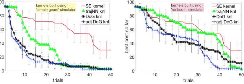
(a) Informed kernels generated using simulator with simplified gear dynamics.
(b) Informed kernels generated using simplified gear dynamics, without boom model.
Figure 7: BO is run on the original simulator. Informed kernels perform well despite significant mismatch, when kernels are generated using simulator with simplified gear dynamics (left). In the case of severe mismatch, when the boom model is also removed, informed kernels still improve over baseline SE (right). Plots show best cost for mean over 50 runs for each algorithm, 95% CIs.
NN-based and DoG-based kernels on both costs shows that the same kernel can indeed be used for optimizing multiple costs robustly, without any further tuning needed.
5.3. Experiments with Increasing Simulation-Hardware Mismatch
In this section, we describe our experiments with increasing simulation-hardware mismatch and its effect on approaches that use information from simulation during hardware opti-mization. The quality of information transfer between simulation and hardware depends not only on the mismatch between the two, but also on the controller used. For a robust controller, small dynamics errors would not cause a significant deterioration in performance, while for a sensitive controller this might be much more detrimental.
In the rest of this section, we provide experimental analyses of settings with increasing simulated mismatch and their effect on optimization of the 50-dimensional VNMC from Section 4.5. We compare several approaches that improve sample-efficiency of BO and investigate if the improvement they offer is robust to mismatch between the simulated setting used for constructing kernel/prior and the setting on which BO is run.
First, we examine the performance of our proposed approaches with informed kernels: kDoG, ktrajNN and kDoGadj. Figure 7a shows the case when informed kernels are generated
using the simulator with simplified gear dynamics while BO is run on the original simulator. After 50 trials, all runs with informed kernels find walking solutions, while for SE only 70% have walking solutions.
Next, Figure 7b shows performance of kDoG,ktrajNN and kDoGadj when the kernels are
constructed using a simulator with simplified dynamics and without a the boom. In this case the mismatch with the original simulator is larger than before and we see the advantage of using adjustment for DoG-based kernel: kDoGadj finds walking points in all runs after 35
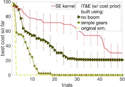
(a) BO with cost prior: straightforward ap-proach useful for low-to-medium mismatch; but no improvement if mismatch is severe.
(b) Performance of IT&E algorithm (our im-plementation of Cully et al. (2015), adapted to bipedal locomotion).
Figure 8: BO using prior-based approaches. Mean over 50 runs for each algorithm, 95% CIs.
of the runs after 50 trials. The performance of SE stays the same, as it uses no prior information from any simulator.
This illustrates that while the original DoG-based kernel can recover from slight simulation-hardware mismatch, the adjusted DoG-kernel is required for higher mismatch. ktrajNNseems to recover from the mismatch, but might benefit from an adjusted version. We leave this to future work.
5.3.1. Comparisons of Prior-based and Kernel-based Approaches
In this section, we classify approaches that use simulation information in hardware optimiza-tion as prior-based or kernel-based. Prior-based approaches use costs from the simulaoptimiza-tion in the prior of the GP used in the BO. This can help BO a lot if the costs are similar between simulation and hardware, and the cost function is fixed. However, in the pres-ence of large mismatch, controllers that perform well in simulation might fail on hardware. A prior-based method can be biased towards sampling promising points from simulation, resulting in worse performance than uninformed BO. Kernel-based approaches consist of methods that incorporate information from simulation into the kernel of the GP. These can be less sample-efficient as compared to prior-based method, but not as likely to be biased towards unpromising regions in the presence of mismatch. They also easily generalize to multiple costs, so that there is no need to re-run simulations for data collection if the cost is changed. This is important because a lot of these approaches can take several days of computation to generate a cost prior or informed kernel. For example, Cully et al. (2015) report taking 2 weeks on a 16-core computer to generate their map.
Figure 8a shows the performance when using simulation cost in the prior during BO. BO with a cost prior created using the original version of the simulator illustrates what would happen in the best case scenario. When the simulator with simplified gear dynamics is used for constructing the prior, we observe significant improvements over uninformed BO prior. However, when the prior is constructed from simplified gear dynamics and no boom setting, the approach performs slightly worse than uninformed BO. This shows that while an informed prior can be very helpful when created from a simulator close to hardware, it can hurt performance if simulator is significantly different from hardware.
Next, we discuss experiments with our implementation of Intelligent Trial and Error (IT&E) algorithm from Cully et al. (2015). This algorithm combines adding a cost prior from simulated evaluations with adding simulation information into the kernel. IT&E de-fines a behavior metric and tabulates best performing points from simulation on their cor-responding behavior score. The behavior metric used in our experiments is duty-factor of each leg, which can go from 0 to 1.0. We discretize the duty factor into 21 cells of 0.05 increments, leading to a 21×21 grid. We collect the 5 highest performing controllers for each square in the behavior grid, creating a 21×21×5 grid. Next, we generate 50 random combinations of a 21×21 grid, selecting 1 out of the 5 best controllers per grid cell. Care was taken to ensure that all 5 controllers had comparable costs in the simulator used for creating the map. Cost of each selected controller is added to the prior and BO is performed in the behavior space, like in Cully et al. (2015).
Figure 8b shows BO with IT&E constructed using different versions of the simulator. IT&E constructed using simplified gear dynamics simulator is slightly less sample-efficient than the straightforward ‘cost prior’ approach. When constructed with the simulator with no boom, IT&E is able to improve over uninformed BO. However, it only finds walking points in 77% of the runs in 50 trials in this case, as some of the generated maps contained no controllers that could walk on the ‘hardware’. This is a shortcoming of the IT&E algorithm, as it eliminates a very large part of the search space and if the pre-selected space does not contain a walking point, no walking controllers can be sampled with BO. This problem could possibly be avoided by using a finer grid, or a different behavior metric. However tuning such hyper-parameters can turn out to be expensive, in computation and hardware experiment time.
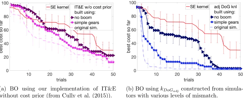
To separate the effects of using simulation information in prior mean vs kernel, we evaluated a kernel-only version of IT&E algorithm (Figure 9a). It shows that the cost prior is crucial for the success of IT&E and performance deteriorates without it. Hence, it is not practical to use IT&E on a cost different than what it was generated for. Nonetheless, Figure 7 showed that BO with adjusted DoG kernel is able to handle both moderate and severe mismatch with kernel-only information, collected in Figure 9b.
ad-(a) BO using our implementation of IT&E without cost prior (from Cully et al. (2015)).
(b) BO usingkDoGadjconstructed from simula-tors with various levels of mismatch.
Figure 9: BO using kernel-based approaches. Mean over 50 runs for each algorithm, 95% CIs.
justed DoG-based kernel performed well in all the tested scenarios, and can reliably improve sample-efficiency of BO even when the mismatch between simulation and hardware is high.
6. Conclusion
In this paper, we presented and analyzed in detail our work from Antonova et al. (2016), Antonova et al. (2017) and Rai et al. (2018). These works introduce domain-specific fea-ture transforms that can be used to optimize locomotion controllers on hardware efficiently. The feature transforms project the original controller space into a space where BO can dis-cover promising regions quickly. We described a transform for bipedal locomotion designed with the knowledge of human walking and a neural network based transform that uses more general information from simulated trajectories. Our experiments demonstrate suc-cess at optimizing controllers on the ATRIAS robot. Further simulation-based experiments also indicate potential for other bipedal robots. For optimizing sensitive high-dimensional controllers, we proposed an approach to adjust simulation-based kernel using data seen on hardware. To study the performance of this, as well as compare our approach to other meth-ods, we created a series of increasingly approximate simulators. Our experiments show that while several methods from prior literature can perform well with low simulation-hardware mismatch (sometimes even better than our proposed approach), they suffer when this mis-match increases. In such cases, our proposed kernels with hardware adjustment can yield reliable performance across different costs, simulators and robots.
Acknowledgments
Appendix A: Implementation Details
In this appendix we provide a summary of data collection and implementation details. Our implementation of BO was based on the framework in Gardner et al. (2014). We used Ex-pected Improvement (EI) acquisition function (Mockus et al., 1978). We also experimented with Upper Confidence Bound (UCB) (Srinivas et al., 2010), but found that performance was not sensitive to the choice of acquisition function. Hyper-parameters for BO were initialized to default values: 0 for mean offset, 1.0 for kernel length scales and signal vari-ance, 0.1 for σn (noise parameter). Hyperparameters were optimized using the marginal
likelihood (Shahriari et al. (2016), Section V-A). For all algorithms, we started optimiz-ing hyperparameters after a low-cost controller was found (to save compute resources and avoid premature hyperparameter optimization). The search space boundaries for controller parameters was designed with physical constraints of the ATRIAS robot in mind.
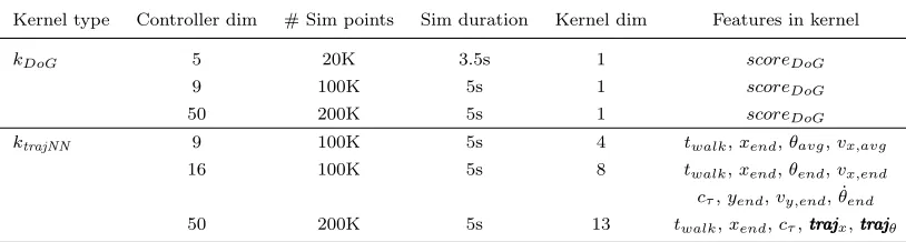
Kernel type Controller dim # Sim points Sim duration Kernel dim Features in kernel
kDoG 5 20K 3.5s 1 scoreDoG
9 100K 5s 1 scoreDoG
50 200K 5s 1 scoreDoG
ktrajNN 9 100K 5s 4 twalk,xend,θavg,vx,avg
16 100K 5s 8 twalk,xend,θend,vx,end
cτ,yend,vy,end, ˙θend
50 200K 5s 13 twalk,xend,cτ,trajtrajtrajx,trajtrajtrajθ
Table 2: Simulation data collection details. scoreDoG was described in Section 3.1.1. For ktrajNN:
twalkis time walked in simulation before falling,xendandyendare thexandypositions of Center of
Mass (CoM) at the end of the short simulation,θis the torso angle, ˙θis the torso velocity,v is the CoM speed (vx is the horizontal andvy is the vertical component),cτ is the squared sum of torques
applied;trajtrajtrajx,trajtrajtrajθdenote vectors with mean CoM andθ measurements every second.
ktrajNN discussed in Section 3.1.2 was constructed by training a fully connected neural
network (NN) with 3 hidden layers, using L1 loss to reconstruct features encoded by tra-jectory summaries. For experiments with 16D controller in Section 5.2, for example, the hidden layers contained 512, 128, 32 units; NN was trained on 100K simulated examples to reconstruct 8D trajectory summaries (see next-to-last row of Table 2). We experimented with various hidden layer sizes for 9D and 50D controllers, but did not find the overall BO performance to be sensitive to size or other training parameters, like NN learning rate. This was likely because NN used to construct an informed kernel only needs to approximately learn to separate well-performing parts from failing parts of the control parameter space. This is the benefit of our choice not to put the output of NN directly into a GP posterior.
References
Rika Antonova, Akshara Rai, and Christopher G Atkeson. Sample efficient optimization for learning controllers for bipedal locomotion. In IEEE-RAS International Conference on Humanoid Robots (Humanoids), pages 22–28. IEEE, 2016.
Rika Antonova, Akshara Rai, and Christopher G Atkeson. Deep Kernels for Optimizing Locomotion Controllers. In Conference on Robot Learning (CoRL), PMLR 78, pages 47–56, 2017.
Zachary Batts, Seungmoon Song, and Hartmut Geyer. Toward a virtual neuromuscular control for robust walking in bipedal robots. In IEEE/RSJ International Conference on Intelligent Robots and Systems (IROS), pages 6318–6323. IEEE, 2015.
Eric Brochu, Vlad M Cora, and Nando De Freitas. A Tutorial on Bayesian Optimization of Expensive Cost Functions, with Application to Active User Modeling and Hierarchical Reinforcement Learning. arXiv preprint arXiv:1012.2599, 2010.
Roberto Calandra, Jan Peters, Carl Edward Rasmussen, and Marc Peter Deisenroth. Man-ifold Gaussian processes for regression. In International Joint Conference on Neural Networks (IJCNN), pages 3338–3345. IEEE, 2016a.
Roberto Calandra, Andr´e Seyfarth, Jan Peters, and Marc Peter Deisenroth. Bayesian Optimization for Learning Gaits Under Uncertainty.Annals of Mathematics and Artificial Intelligence, 76(1-2):5–23, 2016b.
Antoine Cully, Jeff Clune, Danesh Tarapore, and Jean-Baptiste Mouret. Robots that can adapt like animals. Nature, 521(7553):503–507, 2015.
Marc Deisenroth and Carl E Rasmussen. PILCO: A model-based and data-efficient approach to policy search. In International Conference on Machine Learning (ICML), pages 465– 472, 2011.
Peter Englert and Marc Toussaint. Combined Optimization and Reinforcement Learning for Manipulation Skills. In Robotics: Science and Systems, 2016.
Siyuan Feng, Eric Whitman, X Xinjilefu, and Christopher G Atkeson. Optimization-based Full Body Control for the DARPA Robotics Challenge. Journal of Field Robotics, 32(2): 293–312, 2015.
Jacob R Gardner, Matt J Kusner, Zhixiang Eddie Xu, Kilian Q Weinberger, and John Cunningham. Bayesian Optimization with Inequality Constraints. InInternational Con-ference on Machine Learning (ICML), pages 937–945, 2014.
Hartmut Geyer and Hugh Herr. A Muscle-reflex Model that Encodes Principles of Legged Mechanics Produces Human Walking Dynamics and Muscle Activities. IEEE Transac-tions on Neural Systems and Rehabilitation Engineering, 18(3):263–273, 2010.
Christian Hubicki, Jesse Grimes, Mikhail Jones, Daniel Renjewski, Alexander Spr¨owitz, Andy Abate, and Jonathan Hurst. ATRIAS: Design and validation of a tether-free 3D-capable spring-mass bipedal robot. The International Journal of Robotics Research (IJRR), 35(12):1497–1521, 2016.
Verne T Inman, Howard D Eberhart, et al. The major determinants in normal and patho-logical gait. Journal of Bone and Joint Surgery (JBJS), 35(3):543–558, 1953.
Kirthevasan Kandasamy, Gautam Dasarathy, Jeff Schneider, and Barnab´as P´oczos. Multi-fidelity Bayesian Optimisation with Continuous Approximations. In International Con-ference on Machine Learning (ICML), pages 1799–1808, 2017.
Scott Kuindersma, Robin Deits, Maurice Fallon, Andr´es Valenzuela, Hongkai Dai, Frank Permenter, Twan Koolen, Pat Marion, and Russ Tedrake. Optimization-based locomotion planning, estimation, and control design for the atlas humanoid robot. Autonomous Robots, 40(3):429–455, 2016.
Daniel J Lizotte, Tao Wang, Michael H Bowling, and Dale Schuurmans. Automatic Gait Optimization with Gaussian Process Regression. In International Joint Conference on Artificial Intelligence (IJCAI), volume 7, pages 944–949, 2007.
Alonso Marco, Felix Berkenkamp, Philipp Hennig, Angela P Schoellig, Andreas Krause, Stefan Schaal, and Sebastian Trimpe. Virtual vs. real: Trading off simulations and physical experiments in reinforcement learning with Bayesian optimization. In IEEE International Conference on Robotics and Automation (ICRA), pages 1557–1563. IEEE, 2017.
William C Martin, Albert Wu, and Hartmut Geyer. Robust spring mass model running for a physical bipedal robot. InIEEE International Conference on Robotics and Automation (ICRA), pages 6307–6312. IEEE, 2015.
Ruben Martinez-Cantin. Funneled Bayesian optimization for design, tuning and control of autonomous systems. IEEE transactions on cybernetics, (99):1–12, 2018.
J Mockus, V Tiesis, and A Zilinskas. Toward Global Optimization, Volume 2, Chapter: Bayesian Methods for Seeking the Extremum. 1978.
Xue Bin Peng, Glen Berseth, and Michiel van de Panne. Terrain-adaptive locomotion skills using deep reinforcement learning. ACM Transactions on Graphics (TOG), 35(4):81, 2016.
Akshara Rai, Rika Antonova, Seungmoon Song, William Martin, Hartmut Geyer, and Christopher Atkeson. Bayesian optimization using domain knowledge on the ATRIAS biped. In IEEE International Conference on Robotics and Automation (ICRA), pages 1771–1778. IEEE, 2018.
Bobak Shahriari, Kevin Swersky, Ziyu Wang, Ryan P Adams, and Nando de Freitas. Taking the Human Out of the Loop: A Review of Bayesian Optimization. Proceedings of the IEEE, 104(1):148–175, 2016.
Jasper Snoek, Hugo Larochelle, and Ryan P Adams. Practical Bayesian optimization of ma-chine learning algorithms. InAdvances in neural information processing systems (NIPS), pages 2951–2959, 2012.
Jasper Snoek, Kevin Swersky, Rich Zemel, and Ryan Adams. Input warping for Bayesian optimization of non-stationary functions. InInternational Conference on Machine Learn-ing (ICML), pages 1674–1682, 2014.
Seungmoon Song and Hartmut Geyer. A Neural Circuitry that Emphasizes Spinal Feedback Generates Diverse Behaviours of Human Locomotion.The Journal of Physiology, 593(16): 3493–3511, 2015.
Niranjan Srinivas, Andreas Krause, Sham Kakade, and Matthias Seeger. Gaussian process optimization in the bandit setting: no regret and experimental design. In International Conference on Machine Learning (ICML), pages 1015–1022. Omnipress, 2010.
Matthew Tesch, Jeff Schneider, and Howie Choset. Using response surfaces and expected improvement to optimize snake robot gait parameters. In IEEE/RSJ International Con-ference on Intelligent Robots and Systems (IROS), pages 1069–1074. IEEE, 2011.
Nitish Thatte and Hartmut Geyer. Toward Balance Recovery with Leg Prostheses Using Neuromuscular Model Control. IEEE Transactions on Biomedical Engineering, 63(5): 904–913, 2016.
Evangelos Theodorou, Jonas Buchli, and Stefan Schaal. A generalized path integral control approach to reinforcement learning. Journal of Machine Learning Research (JMLR), 11 (Nov):3137–3181, 2010.
Nicolas Van der Noot, Luca Colasanto, Allan Barrea, Jesse van den Kieboom, Renaud Ronsse, and Auke J Ijspeert. Experimental validation of a bio-inspired controller for dynamic walking with a humanoid robot. In IEEE/RSJ International Conference on Intelligent Robots and Systems (IROS), pages 393–400. IEEE, 2015.
Aaron Wilson, Alan Fern, and Prasad Tadepalli. Using Trajectory Data to Improve Bayesian Optimization for Reinforcement Learning. The Journal of Machine Learning Research (JMLR), 15(1):253–282, 2014.
Andrew Gordon Wilson, Zhiting Hu, Ruslan Salakhutdinov, and Eric P Xing. Deep kernel learning. In Artificial Intelligence and Statistics, pages 370–378, 2016.