A Bootstrap Method for Error Estimation
in Randomized Matrix Multiplication
Miles E. Lopes [email protected]
Department of Statistics
University of California at Davis Davis, CA 95616, USA
Shusen Wang [email protected]
Department of Computer Science Stevens Institute of Technology Hoboken, NJ 07030, USA
Michael W. Mahoney [email protected] International Computer Science Institute and Department of Statistics
University of California at Berkeley Berkeley, CA 94720, USA
Editor:Hui Zou
Abstract
In recent years, randomized methods for numerical linear algebra have received growing interest as a general approach to large-scale problems. Typically, the essential ingredient of these methods is some form of randomized dimension reduction, which accelerates computations, but also creates random approximation error. In this way, the dimension reduction step encodes a tradeoff between cost and accuracy. However, the exact numerical relationship between cost and accuracy is typically unknown, and consequently, it may be difficult for the user to precisely know (1) how accurate a given solution is, or (2) how much computation is needed to achieve a given level of accuracy. In the current paper, we study randomized matrix multiplication (sketching) as a prototype setting for addressing these general problems. As a solution, we develop a bootstrap method fordirectly estimatingthe accuracy as a function of the reduced dimension (as opposed to deriving worst-case bounds on the accuracy in terms of the reduced dimension). From a computational standpoint, the proposed method does not substantially increase the cost of standard sketching methods, and this is made possible by an “extrapolation” technique. In addition, we provide both theoretical and empirical results to demonstrate the effectiveness of the proposed method.
Keywords: matrix sketching, randomized matrix multiplication, bootstrap methods
1. Introduction
The development of randomized numerical linear algebra (RNLA or RandNLA) has led to a variety of efficient methods for solving large-scale matrix problems, such as matrix multiplication, least-squares approximation, and low-rank matrix factorization, among others (Halko et al., 2011; Mahoney, 2011; Woodruff, 2014; Drineas and Mahoney, 2016). A general feature of these methods is that they apply some form of randomized dimension reduction to an input matrix, which reduces the cost of subsequent computations. In
c
exchange for the reduced cost, the randomization leads to some error in the resulting solution, and consequently, there is a tradeoff between cost and accuracy.
For many canonical matrix problems, the relationship between cost and accuracy has been the focus of a growing body of theoretical work, and the literature provides many performance guarantees for RNLA methods. In general, these guarantees offer a good qualitative description of how the accuracy depends on factors such as problem size, number of iterations, condition numbers, and so on. Yet, it is also the case that such guarantees tend to be overly pessimistic for any particular problem instance — often because the guarantees are formulated to hold in the worst case among a large class of possible inputs. Likewise, it is often impractical to use such guarantees to determine precisely how accurate a given solution is, or precisely how much computation is needed to achieve a desired level of accuracy.
In light of this situation, it is of interest to develop efficient methods for estimating the exact relationship between the cost and accuracy of RNLA methods on a problem-specific basis. Since the literature has been somewhat quiet on this general question, the aim of this paper is to analyze randomized matrix multiplication as a prototype setting, and propose an approach that may be pursued more broadly. (Extensions are discussed at the end of the paper in Section 6.)
1.1. Randomized matrix multiplication
To describe our problem setting, we briefly review the rudiments of randomized matrix multiplication, which is often known as matrix sketching (Drineas et al., 2006a; Mahoney, 2011; Woodruff, 2014). IfA∈Rn×dandB∈
Rn×d
0
are fixed input matrices, then sketching methods are commonly used to approximateATBin the the regime where max{d, d0} n. For instance, this regime corresponds to “big data” applications where A and B are data matrices with very large numbers of observations.
As a way of reducing the cost of ordinary matrix multiplication, the main idea of sketching is to compute the product ˜ATB˜ of smaller matrices ˜A∈Rt×dand ˜B∈Rt×d0, for some choice of t n. These smaller matrices are referred to as “sketches”, and they are generated randomly according to
˜
A:=SA and B˜ :=SB, (1)
whereS∈Rt×n is a random “sketching matrix” satisfying the condition
E[STS] =In, (2)
withIn being the identity matrix. In particular, the relation (2) implies that the sketched
product is an unbiased estimate, E[ ˜ATB˜] = ATB. Most commonly, the matrix S can be interpreted as acting onA and B by sampling their rows, or by randomly projecting their columns. In Section 2, we describe some popular examples of sketching matrices to be considered in our analysis.
1.2. Problem formulation
Sketch Size t
0 200 400 600 800 1000 1200 1400 1600 1800
L ∞
Norm Error
0 0.05 0.1 0.15 0.2 0.25 0.3 0.35 0.4 0.45 0.5
Sketch Size t
0 200 400 600 800 1000 1200 1400 1600 1800
L ∞
Norm Error
0 0.05 0.1 0.15 0.2 0.25 0.3 0.35 0.4 0.45 0.5
0.99-quantile
Figure 1: Left panel: The curve shows how εt fluctuates with varying sketch size t, as rows are added toS, withA andB held fixed. (Each row of A∈R8,124×112 is a
feature vector of the Mushroom dataset (Frank and Asuncion, 2010), and we set
B= A.) The rows of S were generated randomly from a Gaussian distribution (see Section 2), and the matrixAwas scaled so thatkATAk∞= 1. Right panel:
There are 1,000 colored curves, each arising from a repetition of the simulation in the left panel. The thick black curve represents q0.99(t).
product ˜ATB˜ may be computed quickly, but it is unlikely to be a good approximation to
ATB. Conversely, if t is large, then the sketched product is more expensive to compute, but it is more likely to be accurate. For this reason, we will parameterize the relationship between cost and accuracy in terms of t.
Conventionally, the error of an approximate matrix product is measured with a norm, and in particular, we will consider error as measured by the `∞-norm,
εt :=
ATSTSB−ATB
∞, (3)
wherekCk∞ := maxi,j|cij|for a matrixC= [cij]. (Further background on analysis of`∞
-norm or entry-wise error for matrix multiplication may be found in (Higham, 2002; Drineas et al., 2006a; Demmel et al., 2007; Pagh, 2013), among others.) In the context of sketching, it is crucial to note thatεtis a random variable, due to the randomness inS. Consequently, it is natural to study the quantiles of εt, because they specify the tightest possible bounds
on εt that hold with a prescribed probability. More specifically, for any α ∈ (0,1), the
(1−α)-quantile ofεt is defined as
q1−α(t) := inf
q ∈[0,∞)P εt≤ q
≥ 1−α . (4)
For example, the quantity q0.99(t) is the tightest upper bound on εt that holds with
probability at least 0.99. Hence, for any fixed α, the function q1−α(t) represents a precise tradeoff curve for relating cost and accuracy. Moreover, the function q1−α(t) is specific to the input matricesA and B.
incrementally added to a sketching matrixS, withA andB held fixed. Each time a row is added toS, the sketch sizetincreases by 1, and we plot the corresponding value of εt ast
ranges from 100 to 1,700. (Note that the user is typically unable to observe such a curve in practice.) In the right panel, we display 1,000 repetitions of the simulation, with each colored curve corresponding to one repetition. (The variation is due only to the different draws of S.) In particular, the function q0.99(t) is represented by the thick black curve,
delineating the top 1% of the colored curves at each value oft.
In essence, the right panel of Figure 1 shows that if the user had knowledge of the (unknown) function q1−α(t), then two important purposes could be served. First, for any fixed value t, the user would have a sharp problem-specific bound on εt. Second, for any
fixed error tolerance , the user could select t so that that “just enough” computation is spent in order to achieveεt≤with probability at least 1−α.
The estimation problem. The challenge we face is that a naive computation ofq1−α(t) by generating samples of εt would defeat the purpose of sketching. Indeed, generating
samples of εt by brute force would require running the sketching method many times,
and it would also require computing the entire product ATB. Consequently, the technical problem of interest is to develop an efficient way to estimateq1−α(t), without adding much
cost to asingle run of the sketching method.
1.3. Contributions
From a conceptual standpoint, the main novelty of our work is that it bridges two sets of ideas that are ordinarily studied in distinct communities. Namely, we apply the statistical technique of bootstrapping to enhance algorithms for numerical linear algebra. To some extent, this pairing of ideas might seem counterintuitive, since bootstrap methods are sometimes labeled as “computationally intensive”, but it will turn out that the cost of bootstrapping can be managed in our context. Another reason our approach is novel is that we use the bootstrap to quantify error in the output of a randomized algorithm, rather than for the usual purpose of quantifying uncertainty arising from data. In this way, our approach harnesses the versatility of bootstrap methods, and we hope that our results in the “use case” of matrix multiplication will encourage broader applications of bootstrap methods in randomized computations. (See also Section 6, and note that in concurrent work, we have pursued similar approaches in the contexts of randomized least-squares and classification algorithms (Lopes et al., 2018b; Lopes, 2019).)
From a technical standpoint, our main contributions are a method for estimating the function q1−α(t), as well as theoretical performance guarantees. Computationally, the proposed method is efficient in the sense that its cost is comparable to a single run of standard sketching methods (see Section 2). This efficiency is made possible by an “extrapolation” technique, which allows us to bootstrap small “initial” sketches witht0rows, and inexpensively estimate q1−α(t) at larger valuest t0. The empirical performance of
1.4. Related work
Several works have considered the problem of error estimation for randomized matrix computations—mostly in the context of low-rank approximation (Woolfe et al., 2008; Liberty et al., 2007; Halko et al., 2011), least squares (Lopes et al., 2018b), or matrix multiplication (Ar et al., 1993; Sarl´os, 2006). With attention to matrix multiplication, the latter two papers offer methods for estimating high-probability bounds on the error
ηt := kA˜TB˜ −ATBk, where k · k is either the maximum absolute row sum norm, or the Frobenius norm. At a high level, all of the mentioned papers rely on a common technique, which is to randomly generate a sequence of “test-vectors”, say v1,v2, . . ., and then use the matrix-vector products wi := ˜ATBvi˜ −AT(Bvi) to derive an estimated bound, say ˆ
ηt, for ηt. The origin of this technique may be traced to the classical works (Dixon, 1983;
Freivalds, 1979).
Our approach differs from the “test-vector approach” in some essential ways. One difference arises because the bounds on ˆηt are generally constructed from the vectors {wi}
using conservative inequalities. By contrast, our approach avoids this conservativeness by directly estimating q1−α(t), which is an optimal bound on εt in the sense of equation (4).
A second difference deals with computational demands. For example, in order to compute the vectors {wi} in the test-vector approach, it is necessary to access the full matrices A and B. On the other hand, our method does not encounter this difficulty, because it only requires access to the much smaller sketches ˜A and ˜B. Also, in the test-vector approach, the cost to compute each test-vectorwi is proportional to the large dimension n, while the cost to compute ˆq1−α(t) with our method is independent of n. Finally, the test-vector approach can only be used to check if the product ˜ATB˜ is accurate after it has been computed, whereas our approach can be used to dynamically “predict” an appropriate sketch size tfrom a small “initial” sketching matrix (see Section 3.3).
With regard to the statistics literature, our work builds upon a line of research dealing with “multiplier bootstrap methods” in high-dimensional problems (Chernozhukov et al., 2013, 2014, 2017). Such methods are well-suited to approximating the distributions of statistics such as kx¯k∞, where ¯x ∈ Rp denotes the sample average of n independent mean-zero vectors, with n p. More recently, this approach has been substantially extended to other “max type” statistics arising from sample covariance matrices (Chang et al., 2016; Chen, 2018). Nevertheless, the strong results in these works do not readily translate to our context, either because the statistics are substantially different from the `∞-norm (Chang et al., 2016), or because of technical assumptions (Chen, 2018). For instance, if the results in the latter work are applied to a sample covariance matrix of the form 1
n
Pn
i=1(xi−x¯)(xi−x¯)>, where x1, . . . ,xn ∈ Rp are mean-zero i.i.d. vectors, with x1= (X11, . . . , X1p), then it is necessary to make assumptions such as minj,kvar(X1jX1k)≥c, for some constant c > 0. As this relates to the sketching
context, note that the sketched product may be written as ˜ATB˜ = 1 t
Pt
i=1ATsisTi B, where s1, . . . ,sn ∈Rt are the rows of
√
tS. It follows that analogous variance assumptions would lead to conditions on the matricesAand Bthat could be violated if any column ofAorB
At a more technical level, the ability to avoid restrictions on A and B comes from our use of the L´evy-Prohorov metric for distributional approximations — which differs from the Kolmogorov metric that has been predominantly used in previous works on multiplier bootstrap methods. More specifically, analyses based on the Kolmogorov metric typically rely on “anti-concentration inequalities” (Chernozhukov et al., 2013, 2015), which ultimately lead to the mentioned variance assumptions. On the other hand, our approach based on the L´evy-Prohorov metric does not require the use of anti-concentration inequalities. Finally it should be mentioned that the techniques used to control the LP metric are related to those that have been developed for bootstrap approximations via coupling inequalities as in Chernozhukov et al. (2016).
Outline. This paper is organized as follows. Section 2 introduces some technical background. Section 3 describes the proposed bootstrap algorithm. Section 4 establishes the main theoretical results, and then numerical performance is illustrated in Section 5. Lastly, conclusions and extensions of the method are presented in Section 6, and all proofs are given in the appendices.
2. Preliminaries
Notation and terminology. The set {1, . . . , n} is denoted as [n]. The ith standard basis vector is denoted as ei. If C = [cij] is a real matrix, then kCkF = (Pi,jc2ij)1/2 is
the Frobenius norm, and kCk2 is the spectral norm (maximum singular value). If X is
a random variable and p ≥ 1, we write kXkp = (E[|X|p])1/p for the usual Lp norm. If
ψ : [0,∞) → [0,∞) is a non-decreasing convex function with ψ(0) = 0, then the ψ-Orlicz norm of X is defined as kXkψ := inf{r >0| E[ψ(|X|/r)]≤1}. In particular, we define ψp(x) := exp(xp)−1 forp ≥1, and we say that X is sub-Gaussian when kXkψ2 <∞, or sub-exponential when kXkψ1 <∞. In Appendix F, Lemma 9 summarizes the facts about Orlicz norms that will be used.
We will use cto denote a positive absolute constant that may change from line to line. The matrices A, B, and S are viewed as lying in a sequence of matrices indexed by the tuple (d, d0, t, n). For a pair of generic functionsf andg, we writef(d, d0, t, n).g(d, d0, t, n) when there is a positive absolute constantcso thatf(d, d0, t, n)≤c g(d, d0, t, n) holds for all large values of d, d0, t, and n. Furthermore, if a and b are two quantities that satisfy both
a . b and b . a, then we write a b. Lastly, we do not use the symbols . or when relating random variables.
Examples of sketching matrices. Our theoretical results will deal with three common types of sketching matrices, reviewed below.
• Row sampling. If (p1, . . . , pn) is a probability vector, thenS∈Rt×ncan be constructed by sampling its rows i.i.d. from the set{√1
tp1e1, . . . ,
1 √
tpnen} ⊂R
n, where the vector
1 √
tpiei is selected with probability pi. Some of the most well known choices for the sampling probabilities include uniform sampling, with pi ≡ 1/n, length sampling
(Drineas et al., 2006a; Magen and Zouzias, 2011), with
pi= ke
T
i Ak2keTi Bk2
Pn
j=1keTjAk2keTjBk2
andleverage score sampling, for which further background may be found in the papers (Drineas et al., 2006b, 2008, 2012).
• Sub-Gaussian projection. Gaussian projection is the most well-known random projection method, and is sometimes referred to as the Johnson-Lindenstrauss (JL) transform (Johnson and Lindenstrauss, 1984). In detail, if G ∈ Rt×n is a standard Gaussian matrix, with entries that are i.i.d. samples fromN(0,1), thenS= √1
tGis a
Gaussian projection matrix. More generally, the entries ofGcan be drawn i.i.d. from a zero-mean sub-Gaussian distribution, which often leads to similar performance characteristics in RNLA applications.
• Subsampled randomized Hadamard transform (SRHT). Let n be a power of 2, and define the Walsh-Hadamard matrixHn recursively∗
Hn:=
Hn/2 Hn/2 Hn/2 −Hn/2
with H2:=
1 1
1 −1
.
Next, let D◦n ∈Rn×n be random diagonal matrix with independent ±1 Rademacher
variables along the diagonal, and let P ∈ Rt×n have rows uniformly sampled from
{√1
t/ne1, . . . , 1 √
t/nen}. Then, thet×n matrix
S=P(√1
nHn)D ◦
n (6)
is called an SRHT matrix. This type of sketching matrix was introduced in the seminal paper (Ailon and Chazelle, 2006), and additional details regarding implementation may be found in the papers (Drineas et al., 2011; Wang, 2015). (The factor √1
n is used
so that √1
nHnis an orthogonal matrix.) An important property of SRHT matrices is
that they can be multiplied with any n×dmatrix inO(n·d·logt) time (Ailon and Liberty, 2009), which is faster than the O(n·d·t) time usually required for a dense sketching matrix.
3. Methodology
Before presenting our method in algorithmic form, we first explain the underlying intuition.
3.1. Intuition for multiplier bootstrap method
If the row vectors of √tS are denoted s1, . . . ,st ∈ Rn, then STS may be conveniently expressed as a sample average
STS= 1 t
Pt
i=1sisTi . (7)
For row sampling, Gaussian projection, and SRHT, these row vectors satisfy E[sisTi ] =In.
Consequently, if we define the randomd×d0 rank-1 (dyad) matrix
Di = ATsisTi B, (8)
∗
thenE[Di] =ATB, and it follows that the difference between the sketched and unsketched
products can be viewed as a sample average of zero-mean random matrices
ATSTSB−ATB = 1tPt
i=1(Di−ATB). (9)
Furthermore, in the cases of length sampling and Gaussian projection, the matrices
D1, . . . ,Dt are independent, and in the case of SRHT sketches, these matrices are “nearly” independent. So, in light of the central limit theorem, it is natural to suspect that the random matrix (9) will be well-approximated (in distribution) by a matrix with Gaussian entries. In particular, if we examine the (j1, j2) entry, then we may expect that
eTj1 ATSTSB−ATBej2 will approximately follow the distributionN(0,
1 tσ
2
j1,j2), where the unknown parameterσ2j1,j2 can be estimated with
ˆ
σj21,j2 := 1tPt
i=1 eTj1(Di−A
TSTSB)ej
2
2
.
Based on these considerations, the idea of the proposed bootstrap method is to generate a random matrix whose (j1, j2) entry is sampled from N(0,1tσˆj21,j2). It turns out that an efficient way of generating such a matrix is to sample i.i.d. random variables
ξ1, . . . , ξt∼ N(0,1), independent ofS, and then compute 1
t
Pt
i=1ξi Di−ATSTSB
. (10)
In other words, if S is conditioned upon, then the distribution of the (j1, j2) entry of the above matrix is exactly N(0,1tσˆj2
1,j2).
† Hence, if the matrix (10) is viewed as an
“approximate sample” of ATSTSB−ATB, then it is natural to use the `∞-norm of the matrix (10) as an approximate sample ofεt=kATSTSB−ATBk∞. Likewise, if we define
the bootstrap sample
ε?t :=
1 t
Pt
i=1ξi
Di−ATSTSB
∞, (11)
then the bootstrap algorithm will generate i.i.d. samples ofε?t, conditionally onS. In turn, the (1−α)-quantile of the bootstrap samples, say ˆq1−α(t), can be used to estimateq1−α(t).
3.2. Multiplier bootstrap algorithm
We now explain how proposed method can be implemented in just a few lines. This description also reveals the important fact that the algorithm only requires access to the sketches ˜A and ˜B (rather than the full matrices A and B). Although the formula for generating samples of ε?t given below may appear different from equation (11), it is straightforward to check that these are equivalent. Lastly, the choice of the number of bootstrap samples B will be discussed at the end of subsection 3.3.
†
Algorithm 1 (Multiplier bootstrap for εt).
Input: the number of bootstrap samples B, and the sketches A˜ and B˜.
For b= 1, . . . , B do
1. Draw an i.i.d. sample ξ1, . . . , ξt from N(0,1), independent of S;
2. Compute the bootstrap sampleε?t,b:=
ξ¯·( ˜ATB˜)−A˜TΞB˜
∞, whereξ¯:= 1t Pt
i=1ξi
and Ξ:=diag(ξ1, . . . , ξt).
Return: q1−αˆ (t)←− the (1−α)-quantile of the values ε?t,1, . . . , ε?t,B.
3.3. Saving on computation with extrapolation
In its basic form, the cost of Algorithm 1 isO(B·t·d·d0), which has the favorable property of being independent of the large dimension n. Also, the computation of the samples
ε?t,1, . . . , ε?t,B is embarrassingly parallel, with the cost of each sample being O(t·d·d0). Moreover, due to the way that the quantile q1−α(t) scales with t, it is possible to reduce the cost of Algorithm 1 even further — via the technique of extrapolation (also called Richardson extrapolation) (Sidi, 2003; Brezinski and Zaglia, 2013).
The essential idea of extrapolation is to carry out Algorithm 1 for a modest “initial” sketch sizet0, and then use an initial estimate ˆq1−α(t0) to “look ahead” and predict a larger value t for which q1−α(t) is small enough to satisfy the user’s desired level of accuracy.
The immediate benefit of this approach is that Algorithm 1 only needs to applied to small “initial versions” of ˜A and ˜B, each with t0 rows, which reduces the cost of the algorithm toO(B·t0·d·d0). Furthermore, this means that if Algorithm 1 is run in parallel, then it is
only necessary to communicate copies of the small initial sketching matrices. (To illustrate the small size of the initial sketching matrices, our experiments include several examples where the ratio t0/nis approximately 1/100 or less.)
From a theoretical viewpoint, our use of extrapolation is based on the approximation
q1−α(t) ≈ √κ
t, where t is sufficiently large, and κ = κ(A,B, α) is an unknown number. A
formal justification for this approximation can be made using Proposition 3 in Appendix A, but it is simpler to give an intuitive explanation here. Recall from Section 3.1 that as t becomes large, the (j1, j2) entry [ ˜ATB˜ −ATB]j1,j2 should be well-approximated in distribution by a Gaussian random variable of the form √1
tGj1,j2. In turn, this suggests that
εt should be well-approximated in distribution by √1tmaxj1,j2|Gj1,j2|, which has quantiles that are proportional to √1
t.
In order to take advantage of the theoretical scaling q1−α(t) ≈ √κt, we may use
Algorithm 1 to compute ˆq1−α(t0) with an initial sketch size t0, and then approximate the
valueq1−α(t) for tt0 with the following extrapolated estimator
ˆ
q1−αext(t) := √
t0
√
tq1−αˆ (t0). (12)
Hence, if the user would like to determine a sketch size t so that q1−α(t) ≤ , for some tolerance, thentshould be selected so that ˆq1−αext(t)≤, which is equivalent to
t≥ √
t0
qˆ1−α(t0)
2
In our experiments in Section 5, we illustrate some examples where an accurate estimate of q1−α(t) at t = 10,000 can be obtained from the rule (13) using an initial sketch size
t0 ≈500, yielding a roughly 20-fold speedup on the basic version of Algorithm 1.
Comparison with the cost of sketching. Given that the purpose of Algorithm 1 is to enhance sketching methods, it is important to understand how the added cost of the bootstrap compares to the cost of running sketching methods in the standard way. As a point of reference, we compare with the cost of computingATSTSBwhenSis chosen to be
an SRHT matrix, since this is one of the most efficient sketching methods. If we temporarily assume for simplicity that A and B are both of size n×d, then it follows from Section 2 that computing ATSTSB has a cost of order O(t·d2+n·d·log(t)). Meanwhile, the cost
of running Algorithm 1 with the extrapolation speedup based on an initial sketch size t0 is
O(B·t0·d2). Consequently, the extra cost of the bootstrap does not exceed the stated cost
of sketching when the number of bootstrap samples satisfies
B =O(tt 0 +
nlog(t)
d t0 ), (14)
and in fact, this could be improved further if parallelization of Algorithm 1 is taken into account. It is also important to note that rather small values of B are shown to work well in our experiments, such asB = 20. Hence, as long t0 remains fairly small compared to t, then the condition (14) may be expected to hold, and this is borne out in our experiments. The same reasoning also applies whennlog(t) d·t0, which conforms with the fact that
sketching methods are intended to handle situations wheren is very large.
3.4. Relation with the non-parametric bootstrap
For readers who are more familiar with the “non-parametric bootstrap” (based on sampling with replacement), the purpose of this short subsection is to explain the relationship with the multiplier bootstrap in Algorithm 1. Indeed, an understanding of this relationship may be helpful, since the non-parametric bootstrap might be viewed as more intuitive, and perhaps easier to generalize to more complex situations. However, it turns out that Algorithm 1 is technically more convenient to analyze, and that is why the paper focuses primarily on Algorithm 1. Meanwhile, from a practical point of view, there is little difference between the two approaches, since both have the same order of computational cost, and in our experience, we have observed essentially the same performance in simulations. Also, the extrapolation technique can be applied to both algorithms in the same way.
To spell out the connection, the only place where Algorithm 1 needs to be changed is in step 1. Rather than choosing the multiplier variables ξ1, . . . , ξt to be i.i.d. N(0,1) as
in Algorithm 1, the non-parametric bootstrap chooses ξi = ζi −1, where (ζ1, . . . , ζt) is a
sample from a multinomial distribution, based on tossing t balls into t equally likely bins, whereζi is the number of balls in bini. Hence, the mean and variance of eachξi are nearly
the same as before, withE[ξi] = 0 andvar(ξi) = 1−1/t, but the variables ξ1, . . . , ξtare no
longer independent.
From a more algorithmic viewpoint, it is simple to check that the choice of ξ1, . . . , ξt
and likewise for ˜B. Hence, if S is conditioned upon, then sampling with replacement from the rows of ˜Aand ˜B imitates the random mechanism that originally generated ˜Aand ˜B.
Algorithm 2 (Non-parametric bootstrap for εt). Input: the number of samples B, and the sketches A˜ and B˜.
For b= 1, . . . , B do
1. Draw a vector(i1, . . . , it)by samplingtnumbers with replacement from {1, . . . , t}.
2. Form matrices A˜∗ ∈ Rt×d and B˜∗ ∈ Rt×d
0
by selecting (respectively) the rows from A˜ and B˜ that are indexed by (i1, . . . , it).
3. Compute the bootstrap sample ε∗t,b:=( ˜A∗)T( ˜B∗)−A˜TB˜
∞. Return: qˆ1−α(t)←− the (1−α)-quantile of the values ε∗t,1, . . . , ε∗t,B.
4. Main results
Our main results quantify how well the estimate ˆq1−α(t) from Algorithm 1 approximates
the true value q1−α(t), and this will be done by analyzing how well the distribution of a bootstrap sample ε?t,1 approximates the distribution of εt. For the purposes of comparing distributions, we will use the L´evy-Prohorov metric, defined below.
L´evy-Prohorov (LP) metric. Let L(U) denote the distribution of a random variable
U, and let B denote the collection of Borel subsets of R. For any A ∈ B, and δ > 0, define the δ-neighborhood Aδ :=
x∈R
infy∈A|x−y| ≤δ . Then, for any two random
variables U and V, thedLP metric between their distributions is given by
dLP(L(U),L(V)) := infnδ >0
P(U ∈A)≤P(V ∈A
δ) +δ for all A∈Bo.
The dLP metric is a standard tool for comparing distributions, due to the fact that
convergence with respect to dLP is equivalent to convergence in distribution (Huber and
Ronchetti, 2009, Theorem 2.9).
Approximating quantiles. An important property of the dLP metric is that if two
distributions are close in this metric, then their quantiles are close in the following sense. Recall that ifFUis the distribution function of a random variableU, then the (1−α)-quantile of U is the same as the generalized inverse FU−1(1−α) := inf{q ∈[0,∞)|FU(q)≥1−α}.
Next, suppose that two random variablesU and V satisfy
dLP L(U),L(V)
≤ ,
for some ∈(0, α) withα∈(0,1/2). Then, the quantiles of U andV are close in the sense that
F
−1
U (1−α)−F −1
V (1−α)
≤ ψα(), (15)
be more convenient to express our results for approximating q1−α(t) in terms of the dLP
metric.
4.1. Statements of results
Our main assumption involves three separate cases, corresponding to different choices of the sketching matrix S.
Assumption 1 The dimensions d and d0 satisfy dd0. Also, there is a positive absolute constant κ ≥ 1 such that d1/κ . t . dκ, which is to say that neither d nor t grows
exponentially with the other. In addition, one of the following sets of conditions holds, involving the parameter ν(A,B) :=p
kATAk
∞kBTBk∞.
(a) (Sub-Gaussian case). The entries of the matrix S = [Si,j] are zero-mean i.i.d.
sub-Gaussian random variables, with E[S2i,j] = 1t, and maxi,jk √
tSi,jkψ2 .1. Furthermore,
t & ν(A,B)2/3(logd)5.
(b) (Length sampling case). The matrix S is generated by length sampling, with the probabilities in equation (5), and also, t & (kAkFkBkF)2/3(logd)5.
(c) (SRHT case). The matrix S is an SRHT matrix as defined in equation (6), and also,
t&ν(A,B)2/3(logn)2(logd)5.
Clarifications on bootstrap approximation. Before stating our main results below, it is worth clarifying a few technical items. First, since our analysis involves central limit type approximations of ˜ATB˜ −ATB as a sum of t independent matrices, we will rescale the error variables by a factor of√t, obtaining
Zt:= √
tεt, (16)
as well as its bootstrap analogue,
Zt? :=√tε?t. (17)
With regard to the original problem of estimating the quantileq1−α(t) for εt, this rescaling
makes no essential difference, since quantiles are homogenous with respect to scaling, and in particular, the (1−α)-quantile of Zt is simply
√
tq1−α(t).
As a second clarification, recall that the bootstrap method generates samples ε?t based upon a particular realization of S. For this reason, the bootstrap approximation toL(Zt) is the conditional distribution L(Zt?|S). Consequently, it should be noted that L(Zt?|S) is a random probability measure, and dLP(L(Zt), L(Zt?|S)) is a random variable, since they
Theorem 1 Let h(x) = x1/2 +x3/4 for x ≥ 0. If Assumption 1 (a) holds, then there is an absolute constant c > 0 such that the following bound holds with probability at least 1−1
t − 1 dd0,
dLP
L(Zt), L(Zt?|S) ≤ c·h(ν(A,B))·
p
log(d)
t1/8 .
If Assumption 1 (b) holds, then there is an absolute constant c >0 such that the following bound holds with probability at least 1−1t −dd10,
dLP
L(Zt), L(Zt?|S) ≤ c·h(kAkFkBkF)·
p
log(d)
t1/8 .
Remarks. A noteworthy property of the bounds is that they are dimension-free with respect to the large dimensionn. Also, they have a very mild logarithmic dependence ond. With regard to the dependence ont, there are two other important factors to keep in mind. First, the practical performance of the bootstrap method (shown in Section 5) is much better than what the t−1/8 rate suggests. Second, the problem of finding the optimal rates of approximation for multiplier bootstrap methods is a largely open problem — even in the simpler setting of bootstrapping the coordinate-wise maximum of vectors (rather than matrices). In the vector context, the literature has focused primarily on the Kolmogorov metric (rather than the LP metric), and some quite recent improvements beyond thet−1/8
rate have been developed in Chernozhukov et al. (2017) and Lopes et al. (2018a). However, these works also rely on model assumptions that would lead to additional restrictions on the matrices A and B in our setup. Likewise, the problem of extending our results to achieve faster rates or handle other metrics is a natural direction for future work.
The SRHT case. For the case of SRHT matrices, the analogue of Theorem 1 needs to be stated in a slightly different way for technical reasons. From a qualitative standpoint, the results for SRHT and sub-Gaussian matrices turn out to be similar.
The technical issue to be handled is that the rows of an SRHT matrix are not independent, due to their common dependence on the matrix D◦n. Fortunately, this inconvenience can be addressed by conditioning on D◦n. Theoretically, this simplifies the analysis of the bootstrap, since it “decouples” the rows of the SRHT matrix. Meanwhile, if we let ˜q1−α(t) denote the (1−α)-quantile of the distribution L(εt|D◦n),
˜
q1−α(t) := inf
n
q ∈[0,∞)
P(εt≤q
D◦n)≥1−α o
,
then it is simple to check that ˜q1−α(t) acts as a “surrogate” for q1−α(t), since‡
P(εt≤q˜1−α(t)) =EP εt≤q˜1−α(t)
D◦n
≥E[1−α]
= 1−α.
(18)
‡It is also possible to show that ˜q
1−α(t) fluctuates around q1−α(t). Indeed, if we define the random
variable V := P(εt ≤ q1−α(t)|D◦n), it can be checked that the event V ≥ 1−α is equivalent to the
event ˜q1−α(t) ≤q1−α(t). Furthermore, if we suppose that 1−α lies in the range of the c.d.f. ofεt, then
For this reason, we will view ˜q1−α(t) as the new parameter to estimate (instead ofq1−α(t)),
and accordingly, the aim of the following result is to quantify how well the bootstrap distributionL(Zt?|S) approximates the conditional distribution L(Zt|D◦n).
Theorem 2 Let h(x) = x1/2 +x3/4 for x ≥ 0. If Assumption 1 (c) holds, then there is an absolute constant c > 0 such that the following bound holds with probability at least 1−1
t − 1 dd0 − nc,
dLP
L(Zt|D◦n), L(Zt?|S)
≤ c·h(ν(A,B) log(n))·
p
log(d)
t1/8 .
Remarks. Up to a factor involving log(n), the bound for SRHT matrices matches that for sub-Gaussian matrices. Meanwhile, from a more practical standpoint, our empirical results will show that the bootstrap’s performance for SRHT matrices is generally similar to that for both sub-Gaussian and length-sampling matrices.
Further discussion of results. To comment on the role of ν(A,B) and kAkFkBkF in
Theorems 1 and 2, it is possible to interpret them as problem-specific “scale parameters”. Indeed, it is natural that the bounds ondLP should increase with the scale ofA and Bfor
the following reason. Namely, if A or B is multiplied by a scale factor κ >0, then it can be checked that the quantile error|q1−αˆ (t)−q1−α(t)|will also change by a factor ofκ, and furthermore, the inequality (15) demonstrates a monotone relationship between the sizes of the quantile error and the dLP error. For this reason, the bootstrap may still perform well in relation to the scale of the problem when the magnitudes of the parametersν(A,B) and
kAkFkBkF are large. Alternatively, this idea can be seen by noting that the dLP bounds
can be made arbitrarily small by simply changing the units used to measure the entries of
A andB.
Beyond these considerations, it is still of interest to compare the results for different sketching matrices once a particular scaling has been fixed. For concreteness, consider a scaling where the spectral norms ofAand B satisfykAk2 kBk2 1. (As an example, if
we view A>A as a sample covariance matrix, then the condition kAk2 1 simply means that the largest principal component score is of order 1.) Under this scaling, it is simple to check thatν(A,B) =O(1), and kAkFkBkF =O(
p
r(A)r(B)), wherer(A) :=kAk2 F/kAk22
is the “stable rank”. In particular, note that if A and B are approximately low rank, as is common in applications, then r(A) d, and r(B)d0. Accordingly, we may conclude that if the conditions of Theorems 1 and 2 hold, then bootstrap consistency occurs under the following limits
p
5. Experiments
This section outlines a set of experiments for evaluating the performance of Algorithm 1 with the extrapolation speed-up described in Section 3.3. The experiments involved both synthetic and natural matrices, as described below.
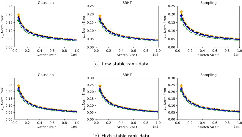
Synthetic matrices. In order to generate the matrixA∈Rn×dsynthetically, we selected the factors of its singular value decompositionA=Udiag(σ)VT in the following ways, fixing
n= 30,000 andd= 1,000. In previous work, a number of other experiments in randomized matrix computations have been designed along these lines (Ma et al., 2014; Yang et al., 2016).
The factor U ∈Rn×d was selected as the Q factor from the reduced QR factorization of a random matrix X ∈ Rn×d. The rows of X were sampled i.i.d. from a multivariate
t-distribution, t2(µ,C), with 2 degrees of freedom, mean µ = 0, and covariance cij =
2×0.5|i−j| whereC= [cij]. (This choice causes the matrix A to have high row-coherence, which is of interest, since this is a challenging case for sampling-based sketching matrices.) Next, the factor V∈Rd×d was selected as the Q factor from a QR factorization of a d×d
matrix with i.i.d. N(0,1) entries. For the singular values σ ∈ Rd+, we chose two options,
leading to either a low or high stable rank r(A) = kAk2F
kAk2
2. In the low stable rank case, we putσi = 10κi for a set of equally spaced valuesκi between 0 and -6, yielding r(A) = 36.7. Alternatively, in the high stable rank case, the entries of σ were equally spaced between 0.1 and 1, yieldingr(A) = 370.1. Finally, to make all numerical comparisons on a common scale, we normalized Aso that kATAk∞= 1.
Natural matrices. We also conducted experiments on five natural data matrices A
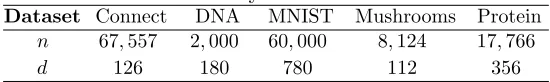
from the LIBSVM repository Chang and Lin (2011), named ‘Connect’, ‘DNA’, ‘MNIST’, ‘Mushrooms’, and ‘Protein’, with the same normalization that was used for the synthetic matrices. These datasets are briefly summarized in Table 1.
Table 1: A summary of the natural datasets.
Dataset Connect DNA MNIST Mushrooms Protein
n 67,557 2,000 60,000 8,124 17,766
d 126 180 780 112 356
5.1. Design of experiments
For each matrix A, natural or synthetic, we considered the task of estimating the quantile
q0.99(t) for the random sketching error εt =
ATA−ATSTSA
∞. The sketching matrix
S∈Rt×n was allowed to be one of three types: Gaussian projection, length-sampling, and SRHT, as described in Section 2.
of the random variable εt. In turn, the 0.99 sample quantile of the 1,000 realizations ofεt
was treated as the true value of q0.99(t), and this appears as the black curve in all plots.
Extrapolated estimates. With regard to the bootstrap extrapolation method in Section 3.3, we fixed the value t0 = d/2 as the initial sketch size to extrapolate from. For eachA, and each type of sketching matrix, we applied Algorithm 1 to each of the 1,000 realizations of ˜A = SA ∈ Rt0×d generated previously. Each time Algorithm 1 was run, we used the modest choice of B = 20 for the number of bootstrap samples. From each set of 20 bootstrap samples, we used the 0.99 sample quantile as the estimate ˆq0.99(t0).§
Hence, there were 1,000 realizations of ˆq0.99(t0) altogether. Next, we used the scaling rule in equation (12) to obtain 1,000 realizations of the extrapolated estimate ˆq0.99ext(t) for values
t≥t0.
In order to illustrate the variability of the estimate ˆq0.99ext(t) over the 1,000 realizations, we plot three different curves as a function of t. The blue curve represents the average value of ˆq0.99ext(t), while the green and yellow curves respectively correspond to the estimates ranking 100th an 900th out of the 1,000 realizations.
5.2. Comments on numerical results
Overall, the numerical results for the bootstrap extrapolation method are quite encouraging, and to a large extent, the method is accurate across many choices of Aand S. Given that the blue curves representingE[ˆq0.99ext(t)] are closely aligned with the black curves forq0.99(t),
we see that the extrapolated estimate is essentially unbiased. Moreover, the variance of the estimate is fairly low, as indicated by the small gap between the green and yellow curves. The low variance is also notable when considered in light of the fact that only B = 20 bootstrap samples are used to construct ˆq0.99ext(t), since the variance should decrease as B
becomes larger.
With attention to the extrapolation rule (12), there are two main points to note. First, the plots show that the extrapolation may be initiated at fairly low values oft0, which are
much less than the sketch sizes needed to achieve a small sketching errorεt. Second, we see that ˆq0.99ext(t) remains accurate for tmuch larger than t0, well up tot= 10,000 and perhaps even farther. Consequently, the results show that the extrapolation technique is capable of saving quite a bit of computation without much detriment to statistical performance.
To consider the relationship between theory and practice, one basic observation is that all three types of sketching matrices obey roughly similar bounds in Theorems 1 and 2, and indeed, we also see generally similar numerical performance among the three types. At a more fine-grained level however, the Gaussian and SRHT sketching matrices tend to produce estimates ˆq0.99ext(t) with somewhat higher variance than in the case of length sampling. Another difference between theory and simulation, is that the actual performance of the method seems to be better than what the theory suggests — since the estimates are accurate at values of t0 that are much smaller than what would be expected from the rates
in Theorems 1 and 2.
§
(a)Low stable rank data.
(b)High stable rank data.
Figure 1: Extra-D1k.
.
2
Figure 2: Results for synthetic matrices. The black line representsq0.99(t) as a function of t. The blue star is the average bootstrap estimate at the initial sketch size
t0 =d/2 = 500, and the blue line represents the average extrapolated estimate
E[ˆq0.99ext(t)] derived from the starting value t0. To display the variability of the estimates, the green and yellow curves correspond to the 100th and 900th largest among the 1,000 realizations of ˆq0.99ext(t) at each t.
6. Conclusions and extensions
In this paper, we have focused on estimating the quantile q1−α(t) as a way of addressing two fundamental issues in randomized matrix multiplication: (1) knowing how accurate a given sketched product is, and (2) knowing how much computation is needed to achieve a specified degree of accuracy. With regard to methodology, our approach is relatively novel in that it uses the statistical technique of bootstrapping to serve a computational purpose — by quantifying the error of a randomized sketching algorithm. A second important component of our method is the extrapolation technique, which ensures that the cost of estimating q1−α(t) does not substantially increase the overall cost of standard sketching
methods. Furthermore, our numerical results show that the extrapolated estimate is quite accurate in a variety of different situations, suggesting that our method may offer a general way to enhance sketching algorithms in practice.
(a)Connect (n= 67,557andd= 126).
(b)DNA (n= 2,000andd= 180).
(c)MNIST (n= 60,000andd= 780).
(d)Mushrooms (n= 8,124andd= 112).
(e)Protein (n= 17,766andd= 356).
Figure 4: Real-extra. 7
At a high level, each of the applications below deals with an object, say Θ, that is difficult to compute, as well as a randomized approximation, say Θ, that is built from ae
sketching matrix S withtrows. Next, if we consider the random error variable
εt=kΘe −Θk,
for an unspecified norm k · k, then the problem of estimating the relationship between accuracy and computation can again be viewed as the problem of estimating the quantile functionq1−α(t) associated withεt. In turn, this leads to the question of how to develop a
new bootstrap procedure that can generate approximate samples ofεt, yielding an estimate ˆ
q1−α(t). However, instead of starting from the multiplier bootstrap (Algorithm 1) as before, it may be conceptually easier to extend the non-parametric bootstrap (Algorithm 2) — because the latter bootstrap can viewed as a “plug-in” procedure that replaces ATB with
˜
ATB˜, and replaces ˜ATB˜ with ( ˜A∗)T( ˜B∗).
• Linear regression. Consider a multi-response linear regression problem, where the rows ofB∈Rn×d0
are response vectors, and the rows ofA∈Rn×d are input observations.
The optimal solution to`2-regression is given by
Wopt = argmin
W∈Rd×d0
AW−B
2
F = (A
TA)†ATB,
which has O(nd2 +ndd0) cost. In the case where max{d, d0} n, the matrix multiplications are a computational bottleneck, and an approximate solution can be obtained via
f
Wopt= ( ˜ATA˜)†( ˜ATB˜),
which has a cost O(td2 +tdd0) + Csketch, where Csketch is cost of matrix
sketch-ing (Drineas et al., 2006b, 2011, 2012; Clarkson and Woodruff, 2013). In order to estimate the quantile function associated with the error variableεt=kWoptf −Woptk,
we could consider generating bootstrap samples of the form ε∗t = kWf∗opt−Wfoptk,
whereWf∗opt = (( ˜A∗)T( ˜A∗))†( ˜A∗)T( ˜B∗). For recent results in the case where W is a
vector, we refer to the paper (Lopes et al., 2018b).
• Functions of covariance matrices. If the rows of the matrixAare viewed as a sample of observations, then inferences on the population covariance structure are often based on functions of the form ψ(ATA). For instance, the function ψ(ATA) could be the
top eigenvector, a set of eigenvalues, the condition number, or a test statistic. In any of these cases, if ψ( ˜ATA˜) is used as a fast approximation (Dasarathy et al., 2015), then the sketching error εt = kψ( ˜ATA˜) −ψ(ATA)k might be bootstrapped using ε∗t =kψ(( ˜A∗)T( ˜A∗))−ψ( ˜ATA˜)k.
• Approximate Newton methods. In large-scale applications, Newton’s method is often impractical, since it involves the costly processing of a Hessian matrix. As an example, consider an optimization problem arising in binary classification, where the rows of
function f(w) = Pn
i=1log 1 +e−yiw
Tx i+γ
2kwk 2
2 over coefficient vectors w in Rd.
The associated Newton step, with step sizeκ, is
w←w−κH−1∇f,
involving the Hessian
H=ATA+γId, where A=diag 1 +ey1w
Tx
1, . . . ,1 +eynwTxn−1X.
If d n, the cost of Newton’s method is dominated by the formation of H
at each iteration, and the Hessian matrix can be approximated by the sketched version ˜H= ˜ATA˜ +γI
d, which reduces the per-iteration cost from O(nd2) to O(td2+nd) +Csketch (Pilanci and Wainwright, 2017; Roosta-Khorasani and Ma-honey, 2016; Xu et al., 2016). In this context, the quality of the approximate Newton step could be assessed in terms of the error
εt=kH˜−1∇f − H−1∇fk,
and in turn, this might be bootstrapped using ε∗t =k( ˜H∗)−1∇f − H˜−1∇fk,where ˜
H∗= ( ˜A∗)T( ˜A∗) +γI d.
Acknowledgments
We thank the anonymous reviewers for their helpful suggestions. MEL thanks the National Science Foundation for partial support under grant DMS-1613218. MWM would like to thank the National Science Foundation, the Army Research Office, and the Defense Advanced Research Projects Agency for providing partial support of this work.
Appendices
Outline of appendices. Appendix A explains the main conceptual ideas underlying the proofs of Theorems 1 and 2. In particular, the proofs of these theorems will be decomposed into two main results: Propositions 3 and 4, which are given in Appendix A.
Appendix B will prove the sub-Gaussian case of Proposition 3, and Appendix C will prove the sub-Gaussian case of Proposition 4. Later on, Appendices D and E, will explain how the arguments can be changed to handle the length-sampling and SRHT cases.
Conventions used in proofs. If either of the matrices A or B are 0, then εt has a
Appendix A. Gaussian and bootstrap approximations
Section A.1 introduces some notation that helps us to analyze the rescaled sketching error
Zt from the viewpoint of empirical processes. Next, in Section A.2, Theorem 1 will be decomposed into two propositions that compareZtandZt? with the maximum of a suitable
Gaussian process. The proofs of these propositions may be found in Appendices B and C.
A.1. Making a link between empirical processes and sketching error
The main idea of our analysis is to viewZt as the maximum of an empirical process, which
we now define. Recall the notation
Di=ATsisTi B and Mi = AT(sisTi −In)B.
Let Gt(·) be the empirical process that acts on linear functions f :Rd×d
0
→ R, according to
Gt(f) :=
1
√ t
t
X
i=1
f(Di)−f(ATB)
= √1 t
t
X
i=1
f(Mi).
For future reference, we also define the corresponding bootstrap process
G?t(f) :=
1
√ t
t
X
i=1
ξi·f(Di)−f ATSTSB
,
whereξ1, . . . , ξt are i.i.d.N(0,1) and independent ofS.
Next, we define a certain collection F of linear functions fromRd×d
0
toR. Letj1∈[d], j2∈[d0], s∈ {−1,1}, and j:= (j1, j2, s). Then, for any matrix W∈Rd×d
0
, we put
fj(W) := s·tr CTj W
,
whereCj:=sej1e
T j2 ∈R
d×d0
and ej1 ∈R
d, e j2 ∈R
d0
are standard basis vectors. In words, the functionfjmerely picks out the (j1, j2) entry ofW, and multiplies by a signs. Likewise, let J be the collection of all the triples j, and define the class of linear functions
F :=
fj |j∈J .
Clearly,card(F) = 2dd0. Under this definition, it is simple to check thatZtandZt?, defined
in equations (16) and (17), can be expressed as
Zt = max fj∈F
Gt(fj), and Zt? = max fj∈F
G?t(fj).
A.2. Statements of the approximation results
Theorems 1 and 2 are obtained by combining the following two results (Propositions 3 and 4) via the triangle inequality. In essence, these results are based on a comparison with the maximum of a certain Gaussian process. More specifically, letG:F →R be a zero-mean Gaussian process whose covariance structure is defined according to
EG(fj)G(fk)
= cov fj(D1), fk(D1)
= E
h
fj(D1)fk(D1)
i
for all j,k∈J. In turn, define the following random variable as the the maximum of this Gaussian process,
Z := max
fj∈F G(fj).
In order to handle the case of SRHT matrices, define another zero-mean Gaussian process ˜
G : F → R (conditionally on a fixed realization of D◦n) to have its covariance structure
given by
EG(˜ fj) ˜G(fk) D◦n
= cov fj(D1), fk(D1) D◦n
= E
h
fj(D1)fk(D1)
D
◦ n
i
−fj(ATB)fk(ATB), (23)
and let ˜Z denote the maximum of the process ˜G,
˜
Z := max
fj∈F ˜ G(fj).
We are now in position to state the approximation results.
Proposition 3 (Gaussian approximation) Under Assumption 1 (a), the following bound holds,
dLP L(Zt),L(Z)
≤ c·ν(A,B) 3/4·p
log(d)
t1/8 .
Under Assumption 1 (b), the following bound holds,
dLP L(Zt),L(Z)
≤ c·(kAkFkBkF) 3/4·p
log(d)
t1/8 .
Under Assumption 1 (c), the following bound holds with probability at least 1−c/n
dLP L(Zt),L( ˜Z|D◦n)
≤ c·ν(A,B)
3/4·(log(n))3/4·p
log(d)
t1/8 .
Proposition 4 (Bootstrap approximation) If Assumption 1 (a) holds, then the follow-ing bound holds with probability at least 1−1t −dd10,
dLP L(Z),L(Zt?|S)
≤ c·ν(A,B) 1/2p
log(d)
t1/8 .
If Assumption 1 (b) holds, then the following bound holds with probability at least1−1t−dd10,
dLP L(Z),L(Zt?|S)
≤ c·(kAkFkBkF) 1/2p
log(d)
t1/8 .
If Assumption 1 (c) holds, then the following bound holds with probability at least 1−1t −dd10 − nc,
dLP L( ˜Z|D◦n),L(Zt?|S)
≤ c·ν(A,B)
1/2·log(n)1/2·p
log(d)
Appendix B. Proof of Proposition 3, part (a)
LetA⊂Rbe a Borel set. Due to Theorem 3.1 from the paper Chernozhukov et al. (2016), we have for any δ >0,
P(Zt∈A)≤P(Z ∈Acδ) +clog 2(d)
δ3√t
Lt+Kt(δ) +Jt(δ)), (24)
where we define the following non-random quantities
Lt := max fj∈F
1
t t
X
i=1
E
h
fj(Mi)
3i
, (25)
Kt(δ) := E
"
max
fj∈F
|fj(M1)|3·1
n
max
fj∈F
|fj(M1)|> δ √
t log(card(F))
o #
, (26)
Jt(δ) := E
"
max
fj∈F
|G(fj)|3·1 n
max
fj∈F
|G(fj)|> δ
√ t log(card(F))
o #
. (27)
The remainder of the proof consists in bounding each of these quantities, and we will establish the following two bounds for allδ >0,
Lt ≤ c ν(A,B)3, (28)
Kt(δ) +Jt(δ) ≤ c
δ√t
log(d)+ log(d)ν(A,B)
3
·exp− δ
√ t c ν(A,B) log2(d)
. (29)
Recall also that card(F) = 2dd0, and dd0 under Assumption 1.
For the moment, we set aside the task of proving these bounds, and consider the choice of δ. There are two constraints that we would like δ to satisfy. First, we would like to choose δ so that the bounds onLt and (Kt(δ) +Jt(δ)) are of the same order. In particular,
we desire
Kt(δ) +Jt(δ) ≤ c ν(A,B)3. (30) Second, with regard to line (24) we would like δ to solve the equation
δ = 1 δ3
log2(d)ν(A,B)3
√
t , (31)
so that the second term in line (24) is of order δ. The idea is that ifδ satisfies both of the conditions (30) and (31), then the definition of the dLP metric and line (24) imply
dLP(L(Z),L(Zt)) ≤ c δ.
To proceed, consider the choice
δ0 := log
1/2(d)ν(A,B)3/4
t1/8 ,
To finish the proof, it remains to establish the bounds (28) and (29). To handleLt, note
that¶
E[|fj(Mi)|3] = kfj(M1)k33
≤ ckfj(M1)k3ψ1, (Lemma 9) (32)
≤ ckBC
T
jA
Tk2 F
kBCT
jATk2
3
, (Lemma 14)
= c
kBCTj ATkF
3
(sincekHk2 =kHkF when His rank-1)
= c
tr BCTj ATACjBT 3/2
= ceTj1ATAej1 ·e
T j2B
TBe j2
3/2
≤ c ν(A,B)3, (33)
which proves the claimed bound in line (28).
Next, regarding Kt(δ), let us consider the random variable
η:= max
fj∈F
|fj(M1)|.
It follows from Lemma 9 (part 4) and Lemma 13 in Appendix F thatKt(δ) can be bounded in terms of the Orlicz normkηkψ1,
Kt(δ)≤c
δ√t
log(card(F))+kηkψ1
3
·exp(− δ √
t
kηkψ1 log(card(F)). To handle kηkψ1, it follows from Lemma 9 (part 3), that
kηkψ1 ≤clog(card(F))·max
fj∈F
kfj(M1)kψ1. (34)
Furthermore, due to the earlier calculation starting at line (32) above,
kfj(M1)kψ1 ≤c ν(A,B). (35) Combining the last few steps, we conclude that
Kt(δ)≤c
δ√t
log(card(F)) + log(card(F))ν(A,B)
3
·exp− δ
√ t
cν(A,B) log2(card(F))
. (36)
Lastly, we turn to bounding Jt(δ). Fortunately, much of the argument for bounding Kt(δ) can be carried over. Specifically, consider the random variable
ζ := max
fj∈F
|G(fj)|.
¶In this step, we use the assumption thatk√tS
Lemma 13 in Appendix F shows that Jt(δ) can be bounded in terms ofkζkψ1,
Jt(δ)≤c
δ√t
log(card(F))+kζkψ1
3
·exp− δ
√ t kζkψ1 log(card(F))
.
Proceeding in a way that is similar to the bound for Kt(δ), it follows from part (3) of
Lemma 9 that
kζkψ1 ≤clog(card(F))·max
fj∈F
kG(fj)kψ1.
Furthermore, for every fj ∈F, the facts in Lemma 9 imply
kG(fj)kψ1 ≤ ckG(fj)kψ2
≤ c
q
var(G(fj))
= c
q
var(fj(D1)) (by definition of G)
≤ ckfj(D1)k2
≤ ckfj(D1)kψ1 (37)
≤ ckfj(D1)−E[fj(D1)kψ1 +c|E[fj(D1)]| = ckfj(M1)kψ1 +c|tr(BC
T
j A)|
≤ c ν(A,B), (38)
where the last step follows from the bounds (32) through (33), and the fact that
|tr(BCT
j A)| ≤ ν(A,B). Consequently, up to a constant factor, Jt(δ) satisfies the same
bound as Kt(δ) given in line (36), and this proves the claim in line (29).
Appendix C. Proof of Proposition 4, part (a)
We will show there is a set of “good” sketching matrices S ⊂Rt×n with the following two properties. First, a randomly drawn sketching matrix S is likely to fall inS. Namely,
P(S∈S)≥1−1t. (39)
Second, whenever the event {S ∈ S} occurs, we have the following bound for any δ > 0 and any Borel set A⊂R,
P
max
fj∈F
G?t(fj)∈A S
≤ Pmax
fj∈F
G(fj)∈Aδ
+ c ν(A,B)·δ tlog(1/4card(F)). (40)
If we set δ to the particular choice δ0 :=t−1/8pν(A,B)· log(card(F)), thenδ0 solves the equation
δ0 = ν(A,B)·δlog(card(F))
Consequently, by the definition of the dLP metric, this implies that whenever the event {S∈S} occurs, we have
dLP L(Zt?|S),L(Z)
≤ c t−1/8pν(A,B)·log(card(F)), (41) and this implies the statement of Proposition 4.
To proceed with the main argument of constructing S and demonstrating the two properties (39) and (40), it is helpful to think ofG?t (conditionally onS) andGas Gaussian
vectors of dimensioncard(F) = 2dd0. From this point of view, we can compare the maxima of these vectors using a result due to Chernozhukov et al. (2016, Theorem 3.2). Under our assumptions, this result implies that for any realization of S, any number δ > 0, and any Borel setA⊂R, we have
P
max
fj∈F
G?t(fj)∈A S
≤ Pmax
fj∈F
G(fj)∈Aδ
+ c
√
∆t(S) log(card(F))
δ ,
where we define the following function of S,
∆t(S) := max (fj,fk)∈F×F
E
G?t(fj)G?t(fk) S
−E
G(fj)G(fk) . (42)
When referencing Theorem 3.2 from the paper Chernozhukov et al. (2016), note that E[G(fj)] = 0 and E[G?t(fj)|S] = 0 for all fj ∈F. To interpret ∆t(S), it may be viewed as
the `∞-distance between the covariance matrices associated with G?t (conditionally on S)
and G.
Using the above notation, we define the set of sketching matrices S ⊂Rn×t according to
S∈S if and only if ∆t(S)≤ √ct·ν(A,B)2·log(card(F)). (43)
Based on this definition, it is simple to check that the proof is reduced to showing that the event {S∈S} occurs with probability at least 1− 1t −dd10. This is guaranteed by the
lemma below.
Lemma 5 Suppose Assumption 1 (a) holds. Then, the event
∆t(S) ≤ c √
t·ν(A,B)
2·log card(F)
occurs with probability at least 1−1t −dd10.
Proof We begin by bounding ∆t(S) with two other quantities (to be denoted ∆0t(S),
∆00t(S)) that are easier to bound. Using the fact that 1tPt
i=1Di = ATSTSB it can be
checked that
EG?t(fj)G?t(fk) S
= 1
t
Pt
i=1fj(Di)fk(Di)
−1 t
Pt
i=1fj(Di)
·1 t
Pt
i=1fk(Di)
.
Similarly, recall from line (22) that
E[G(fj)G(fk)] = E
h
fj(D1)fk(D1) i
From looking at the last two lines, it is natural to define the following zero-mean random variables for any triple i,j,k,k
Qi,j,k:=fj(Di)fk(Di)−E
h
fj(Di)fk(Di) i
,
and
Rt,j := 1t Pt
i=1 fj(Di)−E[fj(Di)]
.
Then, some algebra shows that
EG?t(fj)G?t(fk) S
−E
G(fj)G(fk)
= 1 t
Pt
i=1Qi,j,k
−Rt,j·Rt,k
−E fj(D1)
·Rt,k−Efk(D1)
·Rt,j.
So, if we define the quantities
∆0t(S) := max
(j,k)∈J×J
1 t
t
X
i=1 Qi,j,k
,
∆00t(S) := max j∈J
Rt,j
,
then
∆t(S) ≤ ∆0t(S) + ∆00t(S)2+ 2ν(A,B)·∆00t(S),
where we have made use of the simple bound |E[fj(D1)]| ≤ kATBk∞ ≤ ν(A,B). The
following lemma establishes tail bounds for ∆0t(S) and ∆00t(S), which lead to the statement of Proposition 4.
Lemma 6 Suppose Assumption 1 (a) holds. Then, the event
∆0t(S) ≤ √c
t·ν(A,B)
2·log card(F)
(i)
occurs with probability at least 1−1t, and the event ∆00t(S) ≤ √c
t·ν(A,B)·
q
log card(F)
(ii)
occurs with probability at least 1− 1 dd0. kNote thatQ
i,j,kis a multivariate polynomial of degree-4 in the variablesSi,j, and so techniques based
on moment generating functions, like Chernoff bounds, are not generally applicable to controllingQi,j,k. For instance, ifX∼ N(0,1), then the variableX4 does not have a moment generating function. Handling this
Proof of Lemma 6 (i). Letp >2. Due to part (3) of Lemma 9 in Appendix F, we have
k∆0t(S)kp ≤ card(F)2
1/p
· max
(j,k)∈J×J
1 t Pt
i=1Qi,j,k p . (44)
Note that each variable Qi,j,k has moments of all orders, and when j and kare held fixed, the sequence{Qi,j,k}1≤i≤tis i.i.d. For this reason, it is natural to use Rosenthal’s inequality
to bound the Lp norm of the right side of the previous line. Specifically, the version of Rosenthal’s inequality∗∗ stated in Lemma 10 in Appendix F leads to
1 t Pt
i=1Qi,j,k
p
≤c·p/log(p)t ·max
Pt
i=1Qi,j,k
2,
Pt
i=1kQi,j,kkpp
1/p
. (45)
The L2 norm on the right side of Rosenthal’s inequality (45) satisfies the bound
Pt
i=1Qi,j,k
2 =
q
var(Pt
i=1Qi,j,k)
= √t
q
var(Q1,j,k) = √t
q
var fj(D1)fk(D1)
≤ √t
fj(D1)fk(D1)
2 ≤ √tfj(D1)
4·
fk(D1)
4 (Cauchy-Schwarz) ≤ c√tfj(D1)
ψ1 ·
fk(D1)
ψ1 (Lemma 9)
≤ c√tν(A,B)2,
where the last step follows from the fact
kfj(D1)kψ1 ≤c ν(A,B), (46)
obtained in the bounds (32) through (33).
Next, to handle the Lp norms in the bound (45), observe that
kQ1,j,kkp ≤
fj(D1)fk(D1) p+ E
fj(D1)fk(D1)
≤ 2fj(D1)
2p·
fk(D1)
2p (Cauchy-Schwarz)
≤ c p2fj(D1)
ψ1·
fk(D1)
ψ1 (Lemma 9 in Appendix F)
≤ c p2ν(A,B)2 (inequality (46)).
Hence, the second term in the Rosenthal bound (45) satisfies
Pt
i=1kQi,j,kkpp
1/p
≤ c·p2·t1/p·ν(A,B)2,
∗∗
and as long as the first term in the Rosenthal bound dominates††, i.e.
p2 t1/p. t1/2 (47)
then we conclude that for anyjand k,
1 t
Pt
i=1Qi,j,k
p ≤
c·(p/log(p))·ν(A,B)2
√
t .
Since the previous bound does not depend on jork, combining it with the first step in line (44) leads to
∆0t(S)
p ≤ c·(p/log(p))·card(F)
2/p·ν(A,B)2
√ t .
Next, we convert this norm bound into a tail bound. Specifically, if we consider the value
xp := c·(p/log(p))·card(F)2/p·ν(A,B)
2
√ t ·t
1/p
then Markov’s inequality gives
P ∆0t(S) ≥ xp
≤ k∆0t(S)k p p
xpp ≤
1 t.
Considering the choice of pgiven by
p= log(card(F)),
and noting thatcard(F)1/p=e, it follows that under this choice ofp, xp ≤
c·ν(A,B)2·log(card(F))
√ t
· t1/p
log(p)
.
Moreover, as long as t . card(F)κ for some absolute constant κ ≥ 1 (which holds under
Assumption 1), then the last factor on the right satisfies
t1/p
log(p)
≤ (cardlog(p)(F)1/p)κ = log(log(ecardκ (F)) .1.
So, combining the last few steps, there is an absolute constantcsuch that
P
∆0t(S) ≥ c·ν(A,B)2·log(√ card(F)) t
≤ 1 t,
as needed.
††Under the choice ofp= log(
card(F)) = log(2dd0) that will be made at the end of this argument, it is