A New Method to Derive the EOQ Model
with Defective Items and Known Price
Increase
Kanint Teerapabolarn #1
#
Department of Mathematics, Faculty of Science, Burapha University, Chonburi, 20131, Thailand
Abstract - This paper uses a new method, modified quadratic-geometric mean inequality, to derive the optimal EOQ model with defective items and known price increase when the special order can be placed at the regular time for replenishment. This study also uses 100% inspection policy and the known proportion of defective items is removed prior to storage after the screening process. The method is very simple to derive the optimal EOQ model without derivative.
Keywords Defective item, modified quadratic-geometric mean inequality, known price increase.
I. INTRODUCTION
There have been some studies related to basic EOQ (Economic Order Quantity) model with known price increase, which can be found in [5], [7], [8], [10], etc. These studies have yielded useful results in basic deterministic inventory theory. We know that the basic EOQ model with known price increase was adapted by adding the assumption of known price increase to the basic EOQ model. Therefore, the both models have similarity of assumptions. However, this study focuses on the context of known price increase in [10], especially when the special order can be placed at the regular time for replenishment, the inventory level reached the reorder point 0, that can be briefed as follows.
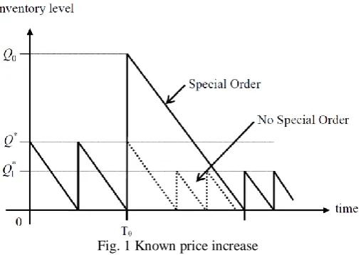
Fig. 1 Known price increase
Assume that, at the present time, the price of an item is c baht and a supplier announces that the price of an item will be increased to be ck baht on the next time. The known price increase situation is depicted in Fig. 1. From which, it follows that unit purchases before and at T0 still cost c baht and purchase quantities before
price increase are Q* units. Unit purchases after T0 will cost ck baht and purchase quantities after price
increase are Q1*(Q*) units. The special order of Q0 units is purchased at T0, when the inventory level reached
the reorder point 0. In this situation, [10] used differential calculus to derive the optimal value of Q0 as follows:
* 2 *
0 *
1
( ) 2
, 2
Q A
Q k
A Q
where * 2AD
Q ic
and *
1 2
,
( )
AD Q
i c k
and the maximum total cost saving is of the form 2
*
* 0
* 1 .
Q G A
Q
(2)
Consider the EOQ model of [10], see (1), this model is appropriate to the case of all items to be perfect quality. In real situation, it is difficult to purchase items with 100% good quality [4]. Thus, in this study we are interested to improve the EOQ of [10] by adding the assumption of defective items of [4] to this model, and using 100% inspection policy and the known proportion of defective items is removed prior to storage after the screening process. Furthermore, in this study we propose a new alternative optimization method, namely modified quadratic-geometric mean inequality, to derive the desired EOQ model.
II. NOTATION, ASSUMPTIONS AND METHOD
The following notation and assumptions are used to derive the desired model.
A. Notation
D demand rate for non-defective items in units per time A ordering cost per order
F the fixed inspection cost per lot
f inspection cost per unit
c purchase cost before the price increase per unit
d the known percentage of defective items in each lot i holding cost fraction per unit per time
k known price increase
*
Q the optimal order quantity before the price increase (includingdefective items)
* 1
Q the optimal order quantity after the price increase (includingdefective items) 0
Q special order quantity (including defective items) *
0
Q the optimal special order quantity (including defective items) s
C total cost when special order is placed n
C total cost when no special order is placed
G total cost saving
*
G the maximum total cost saving
B. Assumptions ([4])
Demand rate is known and constant.
Lead time is equal to zero.
The proportion of defective items in each lot purchased is known and all defective items are removed prior to storage
The inspection cost consists of a fixed inspection cost per lot and a fixed inspection cost per unit, and thescreening time can be ignored.
Time period is infinite.
Shortages are not allowed.
C. Method (the geometric mean and quadratic mean inequality)
It is well known that differential calculus to be a classical optimization method in deterministic inventory theory. In the past few years, some authors have proposed alternative optimization methods, without derivative, to derive their EOQ models such as [3] proposed the algebraic method to derive the basic EOQ model, [6] used the cost comparisons method to derive the basic EOQ model with backorders, [9] used the arithmetic-geometric mean inequality to derive three EOQ models, [1] used the arithmetic-geometric mean inequality together with Cauchy-Bunyakovsky-Schwarz inequality to derive the EOQ model with backorders. In this study, we propose a new alternative optimization method without derivative to derive our EOQ model. The method is defined as follows.
2 2 . 2 a b
ab (3)
The inequality (3) is referred to as the quadratic-geometric mean inequality or the root mean square-geometric mean inequality [2]. It is seen that the inequality (3) can be expressed as
2 2 2
a ab b
(4)
and
2 2 2
a ab b
(5)
if and only if ab. In this context, we will call a new inequality (4) that modified quadratic-geometric mean inequality, which uses to derive the desired EOQ model.
III. RESULT
The aim of this study is a use of modified quadratic-geometric mean inequality to derive the optimal EOQ model with defective items and known price increase.
A. Theoretical result
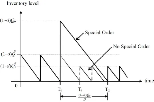
The defective items and known price increase situation is depicted in Fig. 2.
Fig. 2 Defective items and known price increase
The following theorem presents the desired result.
Theorem. The optimal special order quantity, Q0*,is of the form
* 2 *
0 *
1
( ) 2( )
(1 ) ,
2( )
Q A F
Q k d
A F Q
(6)
where * 1 2( )
1
A F D Q
d ic
and
* 1
1 2( )
,
1 ( )
A F D Q
d i c k
and the maximum total cost saving, G*, is 2
*
* 0
*
( ) Q 1 .
G A F Q
(7)
Proof. Let us consider Fig. 2, unit purchases before and at T0 still cost c baht and purchase quantities before
price increase are Q* units, that is,
* 1 2( )
. 1
A F D Q
d ic
(8)
Unit purchases after T0 will cost ck baht and purchase quantities after price increase are Q1* units, that is, *
1
1 2( )
.
1 ( )
A F D Q
d i c k
Note that, the results in (8) and (9) can be easily derived by applying the formula in [4], and it is clear that
* * 1.
Q Q
If special order is placed at T0 of Q0 units then total cost in this case, in time T0 to T2 as shown in Fig. 2,
consists of ordering cost, the inspection cost, items cost and holding cost, that is,total cost when special order is placed Cs 2 2 0 0 0 (1 ) (1 ) 2
ic d Q A F fQ c d Q
D
2 0
0 0 * 2
( )
(1 )
( )
A F Q A F fQ c d Q
Q
(by
2 * 2 (1 )
2 ( )
ic d A F D Q
) (10)
If there is no special order, but all regular orders occur in time T0 to T2 of Q0 units then total cost in time 0
T to T2, see dashed lines in Fig. 2, can be considered to be two parts. The first part, T0 to T1, considers when
the first regular order is placed at T0 of Q* units (c baht). Thus, total cost in this part is equal to 2 * 2
* * (1 ) ( )
(1 )
2
ic d Q A F fQ c d Q
D
2(AF)fQ0c(1d Q) 0 (by (8)). (11)
The second part, T1 to T2, it is seen that purchase quantities in time T1 to T2 of * 0
Q Q units (ck baht) and number of orders is
* * 1 s Q Q Q
. Thus, total cost in this part is equal to
* * 2 * 2
* *
0 0 1
0 0
* *
1 1
( )(1 ) ( )
( ) ( ) ( )(1 )( )
2
Q Q Q Q i c k d Q
A F f Q Q c k d Q Q
D Q Q * * * 0 0 0 * 1
2 Q Q (A F) (c k)(1 d Q)( Q) f Q( Q)
Q
(by (9)). (12)
Therefore, by combining (11) and (12), total cost when no special order is placed
Cn
*
* * 0 * *
0 0
* 1
2(A F) fQ c(1 d Q) 2 Q Q (A F) f Q( Q ) (c k)(1 d Q)( Q )
Q * *
0 0 * 0
1
2(A F) fQ c(1 d Q) 2 Qs Q (A F) k(1 d Q)( Q )
Q
(13)
Hence, total cost saving when special order is placed, G,
G CnCs
* 2
* 0
0 0 * 0 0 0 * 2
1
( )
2( ) (1 ) 2 ( ) (1 )( ) (1 )
( ) s
Q Q A F Q
A F fQ c d Q A F k d Q Q A F fQ c d Q
Q Q * 2 * 0 0 0
* * 2
1
( )
2 ( ) (1 )( )
( )
Q Q A F Q
A F A F k d Q Q
Q Q 2 * 0 0
* 2 *
1
( ) 2( )
(1 ) ( )
( )
A F Q A F
k d Q Q A F
Q Q 2 * 0 0
* 2 * *
1 1
( ) (1 ) 2( )
2 (1 )
2 ( )
A F Q A F k d A F
Q k d Q A F
Q Q Q
(14)
2 * 2
*
* *
1 1
( ) 2( ) 2( )
(1 ) (1 ) .
4( )
Q A F A F
k d k d Q A F
A F Q Q
(15)
The inequality (15) is obtained by looking
2 0 * 2
( )
( )
A F Q Q
and * 0
1
(1 ) 2
2
A F k d Q Q
in (14) to be
2
a and 2ab in (4), respectively. From (14) and (15), it can be seen that the maximum value of G in (14) is obtained if and only if G is equals to the result in (15). By (5), we then have
0 * A FQ Q * * 1 2( )
(1 ) . 2
Q A F
k d A F Q
Thus, the optimal values of Q0 and G* are
Q0*
* 2
* 1
( ) 2( )
(1 )
2( )
Q A F
k d A F Q
and G* 2 * 2 * * * 1 1
( ) 2( ) 2( )
(1 ) (1 ) .
4( )
Q A F A F
k d k d Q A F
A F Q Q
2 * * 1 2( ) (1 ) 2
Q A F
k d A F A F Q
2 * * 1 2( )
( ) (1 ) 1
2( )
Q A F
A F k d
A F Q
2 * 0 * (A F) Q 1 ,
Q
which gives the desired results.
Remark. 1. Consider
2 *
* 0
*
( ) Q 1 ,
G A F Q
because
* * 1,
Q Q we have
* 2 * *
* * *
0 * *
1 1
( ) 2( ) (1 )
(1 ) ,
2( ) 2( )
Q A F Q k d Q
Q k d Q Q
A F Q Q A F
(16)
this implies that
2 *
* 0
*
( ) Q 1 .
G A F A F Q
(17)
Thus, the special order of Q0* units should be purchased when the inventory level is equals to 0 unit.
2. From the result in (16), it is observed that
* * * 0 * * 1 (1 ) 2( )
Q Q k d Q A F Q Q ,
2 ( )
c D
k
c k ic A F
(18)
this implies that
2 *
* 0
*
( ) Q 1
G A F Q
does not depend on d, the known percentage of defective items. 3. Consider the result in the Theorem, if d0, that is, all items are perfect quality. Therefore, the results in the Theorem are the same results in [10] as mentioned in (1) and (2).
4. Because the term of f is not in both formulas of Q0* and G*, thus we can ignore it for computing
numerical results.
B. Numerical results
We give two numerical examples to illustrate numerical results of (6) and (7) in the Theorem.
Example 1. Let demand rate D2,000 units per year, ordering cost A2,000 baht per order, the fixed inspection cost F1,000 baht per lot, holding cost fraction i5% of an item price per year, item price c1,000 baht per unit, known price increase k200 baht per unit and the known percentage of defective items
1%, 5%
d and 10%.
d
*Q
Q
1*Q
*0G
*1% 494.8464 451.7309 8,622.8852
809,379.00 5% 515.6821 470.7512 8,985.9540
10% 544.3311 496.9040 9,485.1737
Example 2. Let demand rate D3,000 units per year, ordering cost A3,000 baht per order, the fixed inspection cost F2,000 baht per lot, holding cost fraction i10% of an item price per year, item price
1,500
c baht per unit, known price increase k300 baht per unit and the known percentage of defective items 5%,
d 10% and 20%.
The optimal special order quantity and the maximum total cost saving for giving d5%, 10% and 20% are as follows:
d
*Q
Q
1*Q
*0G
*5% 470.7512 429.7350 6,831.4715
912,850.85 10% 496.9040 453.6092 7,210.9977
20% 559.0170 510.3104 8,112.3724
From Examples 1 and 2, it is seen that the optimal special order quantity, Q*0, changes along the known
percentage of defective items, d. That is, the optimal special order quantity depends directly on the known percentage of defective items. However, the maximum total cost saving, G*,does not depend on the known percentage of defective items as mentioned in the remark.
IV. CONCLUSION
The new method, modified quadratic-geometric mean inequality, was used to derive the optimal EOQ with defective items and known price increase by assuming that the special order can be placed at the regular time for replenishment, when the inventory level reached the reorder point 0. In addition, the assumption of defective items in [4] was also added to this model by using 100% inspection policy and the known proportion of defective items is removed prior to storage after the screening process. In view of the method of this study, it is a simple alternative optimization method to derive the desired EOQ model without derivative.
ACKNOWLEDGMENT
This work was financially supported by the Research Grant of Burapha University through National Research Council of Thailand (Grant no. 111/2561).
REFERENCES
[1] L. E. Cárdenas-Barrón, “An easy method to derive EOQ and EPQ inventory models with backorders”, Computers and Mathematics with Applications, vol. 59, pp. 948-952, 2010.
[2] Z. Cvetkovski, “Inequalities”. Springer-Verlag, Berlin Heidelberg, 2012.
[3] R. W. Grubbström, “Material Requirements Planning and Manufacturing Resource Planning” (International Encyclopedia of Business and Management), Routledge, . London 1996.
[4] Y. F. Huang, “The EOQ and EPQ models with backlogging and defective items using the algebraic approach”, Journal of Statistics
and Management Systems, vol. 6, pp. 171-180, 2003.
[5] E. Markowski, “EOQ modification for future price increases”, Journal of Purchasing & Materials Management, vol. 22,pp. 28-32, 1986.
[6] S. Minner, S. “ A note on how to compute economic order quantities without derivatives by cost comparisons”, International Journal
of Production Economics, vol. 105, pp. 293-296, 2007.
[7] E. Naddor, “Inventory Systems”, Wiley, New York, 1966.
[8] S. G. Taylor and C. E. Bradley, “Optimal Ordering Strategies for Announced Price Increases”, Operations Research, vol. 33, pp. 312-325, 1985.
[9] J. T. Teng, “ A simple method to compute economic order quantities”, European Journal of Operational Research, vol. 198, pp. 351-353, 2009.