Solving Graphically Sine Wave Second Order Boundary Value Problem using Laplace Transform and Finite Difference Method

(1)

Solving Graphically Sine Wave Second Order

Boundary Value Problem using Laplace

Transform and Finite Difference Method

M.Shalini

#1

, M.Sathyavathy*

2

Assistant Professor & Mathematics, M.Kumarasamy college of Engineering (Autonomou

s

),

Thalavapalayam,Karur, India.

Abstract

In this paper the FDM & LT method has been established for the numerical solution of a two-point

second order boundary value problem’s (BVP) are analyzed. Numerical solutions of both methods were

implemented and are tabulated. Finally it was observed that the finite-difference method is numerically more

strengthen and converges the nearer to LT solution by taking the lengthen intervals.

Keywords

-

Boundary value problem (BVP), Laplace Transform (LT), Finite difference Method (FDM).

I.INTRODUCTION

In Mathematics, Two-point bvp’s have received a major concentration due to its priority in many areas

of sciences and engineering field. Different types of differential equations arise very frequently in optimal

control, aerodynamics, fluid mechanics, chemical–reactor theory, quantum mechanics, reaction-diffusion process

and geophysics .

Different types of logical and computational ideas used for the result of differential equations are given

in the survey literature; Differential Transform Method

[1-6],

Bernoulli Polynomials

[7]

, Adomain

Decomposition Method

[8-13]

, Block Method

[14-16]

, Modified Picard Technique

[17]

, Sinc Collocation

Method

[18],

Runge-kutta 4

th

Order Method

[19]

, Cubic Spline Method

[20]

, Homotopy Perturbation Method

[21-23]

.

In this Paper, we use FDM for the result of two-point boundary value problems has been extensively

used

[24-27]

. In the example problems the step length is elongated and it is examined that the access strengthen

the convergence of the result when compared with the explicit from Laplace Transforms (which gives a close

form of solution), see Table 1.

II.EVALUATION OF FDM

Consider the second order BVP as,

𝝌

′′

+ 𝒔 𝝔 𝝌

′

+ 𝒕 𝝔 𝜻 = 𝒖 𝝔 , 𝝔 ∈ 𝜸, 𝜹

(1)

With the boundary conditions

𝜻 𝜸 = 𝐌 𝐚𝐧𝐝 𝜻 𝜹 = 𝚴

(2)

The period

𝒗, 𝒘

is partitioned into into

𝑛

equal subintervals. The subintervals length is denoted as

ℎ

,

i.e)

𝒉 =

𝜹−𝜸

𝒏

(3)

Let us examine the following points

𝜸 = 𝝔

_𝟎

, 𝝔

_𝟏

= 𝝔

_𝟎

+ 𝒉, 𝝔

_𝟐

= 𝝔

_𝟎

+ 𝟐𝒉, … … . . 𝝔

_𝒎

= 𝝔

_𝟎

+ 𝒎𝒉, … … . , 𝝔

_𝒏

= 𝝔

_𝟎

+ 𝒏𝒉

(4)

The analytical solution at any point

𝝋

𝒎

is indicated by

𝜻

𝒎

and abstract solution is denoted as

𝝌 𝝔

𝒎

.

The Central difference approximation for the differential equation is given below

𝜒𝑚′=_2ℎ1 𝜒𝑚 +1−𝜒𝑚

𝜒𝑚′′=_{ℎ 2}1 𝜒𝑚 +1−2𝜒𝑚+𝜒𝑚 −1

(5)

Substitute (5) in (1)

_ℎ12

𝜒

𝑚 +1

− 2𝜒

𝑚

+ 𝜒

𝑚 −1

+ 𝑠 𝜚

1

2ℎ

𝜒

𝑚 +1

− 𝜒

𝑚

+ 𝑡 𝜚 𝜒

𝑚

= 𝑢 𝜚

(6)

2 𝜒

𝑚 +1

− 2𝜒

𝑚

+ 𝜒

𝑚 −1

+

ℎ 𝑠 𝜚 𝜒

𝑚 +1

− 𝜒

𝑚 −1

+ 2ℎ

2

𝑡 𝜚 𝜒

𝑚

= 2ℎ

2

𝑢 𝜚

(7)

Equation (7) can be written as

(2)

Where

𝑖

𝑚

= 2 −

ℎ 𝑠(𝜚)

𝑗

_𝑚

= −4 + 2ℎ

2

_𝑡(𝜚)

𝑘

_𝑚

= 2 +

ℎ 𝑠(𝜚)

𝑙

_𝑚

= 2ℎ

2

_𝑤(𝜚)

(9)

The following equations are obtained from (8)

𝑖

₁

𝜒

₀

+ 𝑗

₁

𝜒

₁

+ 𝑘

₁

𝜒

₂

= 𝑙

(10)

𝒊

𝟐

𝝌

𝟏

+ 𝒋

𝟐

𝝌

𝟐

+ 𝒌

𝟐

𝝌

𝟑

= 𝒍

𝟐

(11)

etc.

Hence the result of the above equations to a logical order of equations of the form

𝐴𝜒 = 𝑙

for the undistinguished

𝜒

₁

, 𝜒

₂

, 𝜒

₃

, … . 𝜒

_𝑛−1

, where

𝐴

is the co-efficient matrix determine the logical order of equations above provide

the results of the bvp’s.

III.NUMERICAL EXAMPLES

A. Problem 3.1:

Evaluate the two-point BVP of χ

′′

𝜚 +

χ

𝜚 = 0,

χ

′

0 = 1,

χ

_{𝜋 2}

= 0

, by Laplace transform and

Finite difference method.

Solution:

Given:

χ

′′

_{ϱ + χ ϱ = 1, χ}

′

0 = 1, χ π 2

= 0

(12)

The general solution of (12) is

χ ϱ = sin ϱ

(13)

Solving by Laplace Transform

Equation (12) gives

L χ

′′

_{+ L χ = L 0}

₍₁₄₎

s

2

_{χ − sχ 0 − χ}

′

_{0 + χ = 0}

₍₁₅₎

Let

L χ 0

=

ς

(16)

Substituting equation (16) in (15), we get

s

2

_{χ − sχ 0 − 1 + χ = 0}

₍₁₇₎

And simplifying, we obtain

χ =

sς

s2₊₁

+

1

s2₊₁

(18)

Converting into partial fraction ,

χ ω =

sς

s2₊₁

+

𝟏

𝐬𝟐_+𝟏

(19)

Taking inverse Laplace transform

χ ω = sinϱ + ςcosϱ

(20)

Using

_{χ π 2}

= 0

, we obtain

0 = sin

π

2

+ ςcos

π

2

(21)

Which gives

ς = 0

, then

χ ϱ = sin ϱ + 0 cos ϱ

(22)

Then,

𝛘 𝛠 = 𝐬𝐢𝐧 𝛠

(23)

Which is explicit solution

Solving by Finite difference Method

The following steps are written using equation

(12)

i.e)

n = 10 , h =

ν−υ

10

=

π 2 −0 10

=

π

20

(24)

From the above we have

χ 0 = 1, χ π 20

=? , χ 2π 20

=? , … … … χ π 2

= 0

(25)

Equation (12) is expressed by central difference approximations as follows

400

π2

χ

m+1

− 2χ

m

+ χ

m−1

+ χ

m

= 0

(26)

(3)

m = 2 ∶ 400χ

1

+ (−800 + π

2

)χ

2

+ 400χ

3

= 0

(28)

m = 3 ∶ 400χ

2

+ (−800 + π

2

)χ

3

+ 400χ

4

= 0

(29)

:

m = 9 ∶ 400χ

10

+ (−800 + π

2

)χ

9

+ 400χ

8

= 0

(30)

Deriving the logical of equations (27-30) gives the result of the bvp’s; and the comparison with the nearer form

result is presented in table 1.

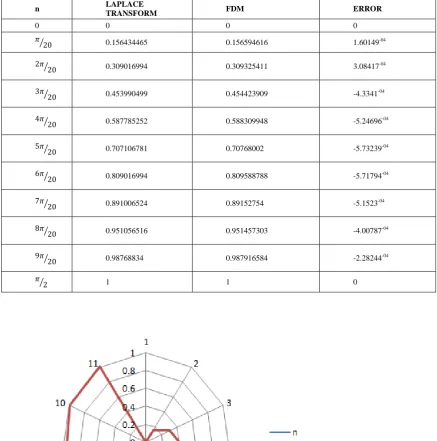
IV. Table 1 NUMERICAL SOLUTION OF PROBLEM

1

n LAPLACE

TRANSFORM FDM ERROR

0 0 0 0

𝜋

20 0.156434465 0.156594616 1.60149-04

2𝜋

20 0.309016994 0.309325411 3.08417-04

3𝜋

20 0.453990499 0.454423909 -4.3341-04

4𝜋

20 0.587785252 0.588309948 -5.24696-04

5𝜋

20 0.707106781 0.70768002 -5.73239-04

6𝜋

20 0.809016994 0.809588788 -5.71794-04

7𝜋

20 0.891006524 0.89152754 -5.1523-04

8𝜋

20 0.951056516 0.951457303 -4.00787-04

9𝜋

20 0.98768834 0.987916584 -2.28244-04

𝜋

2 1 1 0

(4)

Fig 2: n value and FDM

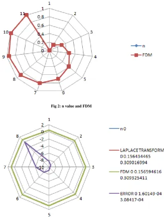
Fig 3: Comparison of n value, LT, FDM and Error

V.CONCLUSION

In this paper, LTM and FDM technique are proposed to solve two point boundary value problems. The

step length is extended in FDM to enhance the convergence of the method; the results are compared with the

close form solution of LT in table

ACKNOWLEDGEMENT

This work was supported by

Ms.M.sathyavathy. I hereby take the opportunity to thank her, who helped me

to make this paper. and also we wish to thank our administrative assistance.

REFERENCES

[1] A.A. Opanuga, J.A. Gbadeyan, S.A. Jyase and H.I. Okagbue, “Effect of Thermal Radiation on the Entropy Generation of

Hydromagnetic Flow through Porous Channel”, the Pacific Journal of Science and Technology, vol. 17, no 2, pp. 59-68, 2016.

[2] M. El-Shahed, “Application of Differential Transform Method to non Linear Oscillatory Systems”, Communication in Nonliear

Simulation,Vol. 13, pp. 1714-1720, 2008.

[3] A.A.Opanuga, o.o.agboola, H.I.Okagbue, “Approximate Solution of Multipoint Boundary Value Problems”, Journal of Engineering

and Applied Sciences, Vol. 10,no 4, pp. 85-89,2015.

[4] J.Biazar and M.Eslami, “Analytic Solution for Telegraph Equation by Differential Transform Method”, Physics Letters a, Vol. 374,

2010, pp. 2904-2906. doi:10.0.16/jphysleta.2010.05.012

(5)

[6] A.A.Opanuga, H.I.Okagbue, S.O.Edeki and O.O.Agboola “Differential Transform Technique for Higher order Boundary Value Problems”, Modern Applied Science, vol. 9, no 13, pp. 224 230, 2015

[7] MD Shafiqul Islam and Afroza Shirin, “Numerical Solution of a Class of Second Order boundary Value Problems on using Bernoulli

Polynomials”, Applied Mathematics, Vol. 2, pp. 1059-1067, 2011. doi:10.4236/am.2011.29147.

[8] G. Adomian, “Solving Frontier Problems of Physics, the Decomposition Method” , Boston, Kluwer Academic 1994.

[9] G. Adomian, “Nonlinear Stochastic Systems and Application to Physics”, Kluwer Academic. the Netherland, 1989.

[10] S. O. Adesanya, E. S. Babadipe and s. A. Arekete, a “New Result on Adomian Decomposition Method for Solving Bratu’s Problem”,

Mathematical Theory and Modeling, vol. 3, no 2, pp. 116-120, 2013.

[11] M. Tatari and M. Dehghan, “The use of the Adomian Decomposition Method for Solving Multipoint Boundary Value Problems”,

Phys. Scr. vol. 73, pp. 672-676, 2006. doi:10.1088/0031 8949/73/6/023

[12] R. Jebari, I. Ghanmi and a. Boukricha, “Adomian Decomposition Method for Solving Nonlinear Heat Equation with Exponential

Nonlinearity”, int. Journal of Maths. Analysis, Vol. 7, no 15, pp. 725-734, 2013

[13] M. Paripoura, E. Hajiloub, A. Hajiloub, H. Heidarib, “Application of Adomian Decomposition Method to Solve Hybrid Fuzzy

Differential”, Journal Of Taibah University For Science, vol. 9, pp. 95–103, 2015.

[14] Z. Omar and j. O. Kuboye, “derivation of block methods for solving second order ordinary differential equations directly using

direct integration and collocation approaches”, indian journal of science and technology, vol. 8, no 12, 2015. Doi: 10.17485/ijst/2015/v8i12/70646

[15] J. O. Kuboye and z. Omar, “new zero-stable block method for direct solution of fourth order ordinary differential equations”, indian

journal of science and technology, vol. 8, no 12, 2015. Doi: 10.17485/ijst/2015/v8i12/70647

[16] T. A. Anake, d. O. Awoyemi and a. O. Adesanya, “one-step implicit hybrid block method for the direct solution of general second

order ordinary differential equations”, iaeng international journal of applied mathematics, vol. 42, no 4, pp. 224 -228, 2012.

[17] H. A. El-arabawy and i. K. Youssef, “a symbolic algorithm for solving linear two-point boundary value problems by modified picard

technique”, mathematica and computer modelling, vol. 49, pp. 344-351, 2009.

[18] B. Bialecki, “sinc-collocation methods for two point boundary value problems”, the ima journal of numerical analysis, vol. 11, no

3, pp. 357-375, 1991. Doi:10.1093/imanum/11.3.357

[19] Anwar ja'afar mohamad-jawad, “second order nonlinear boundary value problems by four numerical methods”, eng &tech journal,

vol. 28, no 2, pp. 1-12, 2010.

[20] E. A. Al-said, “cubic spline method for solving two point boundary value problems”, korean journal of computational and applied

mathematics”, vol. 5, pp. 759-770, 1998. Doi:10.1016/j.mcm.2008.07.030

[21] A. A. Opanuga, o. O. Agboola, h. I. Okagbue, g. J. Oghonyon, “solution of differential equations by three semi-analytical

techniques”, international journal of applied engineering research, vol. 10, no 18, pp. 39168-39174, 2015.

[22] S. Abbasbandy, “iterated he’s homotopy perturbation method for quadratic riccati differential equation”, appl. Math. Comput., vol.

175, pp. 581-589, 2006. Proceedings

[23] D. D. Ganji and a. Sadghi, “application of homotopy-perturbation and variational iteration methods to nonlinear heat transfer and

porous media equations”, journal of computational and applied mathematics, vol. 207, pp. 24-34, 2007.

[24] E.u. Agom and a.m. Badmus, “correlation of adomian decomposition and finite difference methods in solving nonhomogeneous

boundary value problem”, the pacific journal of science and technology, vol. 16, no 1, pp. 104-109, 2015

[25] S. R. K. Iyengar and r. K. Jain, “numerical methods”, new age international publishers, 2009, new delhi, india.

[26] M. L. Dhumal1, s. B. Kiwne, “finite difference method for laplace equation”, international journal of statistika and mathematika, vol.

9, no 1, pp. 11-13, 2014.

[27] Rajkumar meel, yogesh kandhalwal et.al, “a comparative study of boundary value problem with iterative method”, ijmtt, 2017,