Abstract—High Voltage Circuit Breaker’s working base is the electric arc that appears between their contacts when establishing or interrupting the electric current in the circuit. This electric arc is a complex phenomenon where lots of physic interactions take place in a very short time. Over the years, as our knowledge of the interrupting process progressed, many techniques have been developed to test the circuit breakers and simulated arc model. In this paper, modeling of the electric arc and models of high voltage circuit breakers Kema, Schwarz, Schavemaker has been studied. Using the concept of negative feedback, and use a new method to improve the break situation of the breaker on Schavemaker model is presented and results have been extracted. Finally, current and voltage indicators breaker for different modes were compared and showed that models with negative feedback Schavemaker the above methods will produce the best performance.
IndexTerms—High Voltage Circuit breaker, Electric Arc Model, Schavemaker Arc Model, Cassie-Mayr Arc Model, Negative Feedback.
I.INTRODUCTION
Circuit-breakers are very important electric power transmission equipment related to quality of service, because they can isolate faults that otherwise could cause total power system breakdowns. When circuit breaker contacts separate to initiate the interruption process, an electrical arc of extremely high temperature is always produced and becomes the conducting medium in which current interruption will occur. With modern high-voltage breakers, the arc is blown with gas in the same way as a match is blown out with your breath, but with 100 million times the blowing power.
In simple terms, circuit-breakers consist of a plug that is in connection with a contact when the breaker is closed. The current then flows right through the breaker. To interrupt the current, the plug and the contact is separated with rather high speed, resulting in an electric arc in the contact gap between the plug and the contact. This is illustrated in Figure:1 Since
Manuscript received Feb, 2016.
S. Pasumpon, UG Student, Department of EEE, PSN College of Engg. and Tech., Tirunelveli, Tamilnadu.
R. Saravanan, UG Student, Department of EEE, PSN College of Engg. and Tech., Tirunelveli, Tamilnadu.
A. Maruthu, UG Student, Department of EEE, PSN College of Engg. and Tech., Tirunelveli, Tamilnadu.
A.Saravanan, Assistant Professor, Department of EEE, PSN College of Engg. and Tech., Tirunelveli, Tamilnadu.
M.Muneeswaran, Assistant Professor, Department of EEE, PSN College of Engg. and Tech., Tirunelveli, Tamilnadu.
short-circuit currents in most high-voltage power systems frequently reach 50 to 100 kilo amperes, the consequent arc temperature goes beyond 10,000 degrees (C), which is far above the melting point of any known material.
In this paper the characteristics of the electric arc are described with the aim of characterizing the interruption process in high voltage devices. In addition, an overview of the most important models and simulation methods using MATLAB are exposed. [1-2]
Fig.1. Simplification of contact gap
II.ELECTRICARCEVENTINHIGHVOLTAGECIRCUIT BREAKER
The electric arc in a circuit breaker plays the key role in the interruption process and is therefore often addressed as switching arc. The electric arc is a plasma channel between the breaker contacts formed after a gas discharge in the extinguishing medium. When current flows through a circuit breaker and the contacts of the breaker part, driven by the mechanism, the magnetic energy stored in the inductances of the power system forces the current to flow. Just before contact separation, the breaker contacts touch each other at a very small surface area and the resulting high current density makes the contact material to melt. The melting contact material virtually explodes and this leads to a gas discharge in the surrounding medium either air, oil, or SF6. Physically, the arc is an incandescent gas column, with an approximate straight trajectory between electrodes (anode and cathode) and temperatures over 6000 and 10000 ºC. Metallic contact surfaces are also incandescent and a reduction in the cross section of the arc is observed near them. This way, three regions can be defined: a central zone or arc column and the anode and the cathode regions (Figure 2). [3].
Evaluation of High-Voltage Circuit Breaker
Performance with Modified Schavemaker Arc
Model
Fig. 2.The arc channel can be divided into an arc column, a cathode, and an anode region.
From the arc channel, the potential gradient and the temperature distribution can be measured. Figure 3 shows a typical potential distribution along the arc channel between the breaker contacts.
Fig.3. Typical potential distribution along an arc channel.
The peak temperature in the arc column can range from 7000–25000 K, depending on the arcing medium and configuration of the arcing chamber.
The role of the cathode, surrounded by the cathode region, is to emit the current-carrying electrons into the arc column. A cathode made from refractory material with a high boiling point, (e.g. carbon, tungsten, and molybdenum) starts already with the emission of electrons when heated to a temperature below the evaporation temperature this is called thermionic emission. Current densities that can be obtained with this type of cathode are in the order of 10000 A/cm2. The cooling of the heated cathode spot is relatively slow compared with the rate of change of the transient recovery voltage, which appears across the breaker contacts after the arc has extinguished and the current has been interrupted.
A cathode made from non-refractory material with a low boiling point, such as copper and mercury, experience significant material evaporation. These materials emit electrons at temperatures too low for thermionic emission and the emission of electrons is due to field emission. Because of the very small size of the cathode spot, cooling of the heated spot is almost simultaneous with the current decreasing to zero. The current density in the cathode region is much higher than the current density in the arc column itself. This results in a magnetic field gradient that accelerates the gas flow away from the cathode. This is called the Maecker effect.
The role of the anode can be either passive or active. In its passive mode, the anode serves as a collector of electrons leaving the arc column. In its active mode the anode evaporates, and when this metal vapor is ionized in the anode region, it supplies positive ions to the arc column. Active anodes play a role with vacuum arcs: for high current densities, anode spots are formed and ions contribute to the plasma. This is an undesirable effect
because these anode spots do not stop emitting ions at the current zero crossing. Their heat capacity enables the anode spots to evaporate anode material even when the power input is zero and thus can cause the vacuum arc not to extinguish. Directly after contact separation, when the arc ignites, evaporation of contact material is the main source of charged particles. When the contact distance increases, the evaporation of contact material remains the main source of charged particles for the vacuum arcs. For high-pressure arcs burning in air, oil, or SF6, the effect of evaporation of contact material becomes minimal with increasing contact separation, and the plasma depends mainly on the surrounding medium. [1-3, 5]
III.IMPLEMENTATIONOFTHE ARC MODEL BLOCKSET
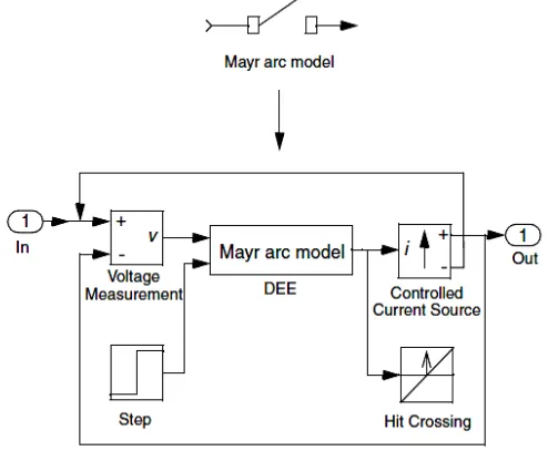
The arc models have been modelled as voltage controlled current sources. This approach is visualized in fig. 4, where both the Mayr arc model block and the underlying system are shown. Some of the elements in fig. 4 will be clarified hereunder.
Fig.4. Implementation of the Mayr arc model.
IV. DEE: Differential Equation Editor
The equations of the Mayr arc model have been incorporated by means of the Simulink DEE (Differential Equation Editor) block, as shown in fig. 5.
Therefore, the following system of equations is solved:
x(1) - the state variable of the differential equation which is the natural logarithm of the arc conductance: ln(g).
x0 - the initial value of the state variable, i.e. the initial value of the arc conductance: g(0).
u(1) - the first input of the DEE block which is the arc voltage: u.
u(2) - the second input of the DEE block which represents the contact separation of the circuit breaker: u(2) = 0 when the contacts are closed and u(2) = 1 when the contacts are being opened.
y-the output of the DEE block which is the arc current: i.
u - the arc voltage
i - the arc current
τ - the arc time constant
P - the cooling power
τ and P are the free parameters of the Mayr arc model which can be set by means of the dialog, as depicted in fig.6, that appears when the Mayr arc model block is double clicked.
Fig. 5. Mayr equation in the Simulink Differential Equation Editor
Fig. 6.Mayr arc model dialog
V. Hit Crossing
The Simulink ‘Hit crossing’ block detects when the input, in this case the current, crosses the zero value. Therefore, by adjusting the stepsize, the block ensures that the simulation finds the zero crossing point. This is of importance while the voltage and current zero crossing ofthe circuit breaker, which behaves as a non-linearresistance, is a crucial moment in the interruption process,that should be computed accurately.
VI. Step
The Simulink ‘Step’ block is used to control the contact separation of the circuit breaker. A step is made from a value zero to one at the specified contact separation time. When the contacts are closed, the following differential equation is solved:
Therefore, the arc model behaves as a conductance with the value g (0). Starting from the contact separation time, the Mayr equation is solved:
Both the initial value of the arc conductance g (0) and the time at which the contact separation of the circuit breaker starts, are specified by means of the arc model dialog, as displayed in fig. 6.
VII. ARC MODELAND TEST CIRCUIT
In this section, the differential equation governing the model Kema, Schwarz, Schavemaker and Negative feedback method applying in the model of Schavemaker and Single phase test circuit is also studied and compared to models that have been proposed.
A. Kema Arc Model
It was derived from three modified Mayr arc model inseries. The equations of this model are as follows [7].
Where, gn is the conductance of the n-th arc, un is the voltage across the n-th arc, τn is time constant arc n-th, An constant cooling curve n i, Kn parameters free, λn Control Cassie - mayr arc n-th , where λ=1arch Cassie and λ=2 Mayr arc results, we also:
B. Schavemaker Arc Model
Differential equation for this model is as follows [6].
Cooling constant P0, P1 constant cooling, which was zero when the current passes through zero, u-arc is arc voltage constant in high current areas and in this study is assumed to be 1100 volts.
This equation shows a clear conformity with the Cassie arc model. At current zero, the above equation reduces to the following differential equation.
This is exactly the Myar arc model.
C. Schwarz Arc Model
This model, a model that is modified Mayr arc time constant and power steering cooling is dependent on the differential equation for this model is as follows [6].
D. Single Phase Test Circuit
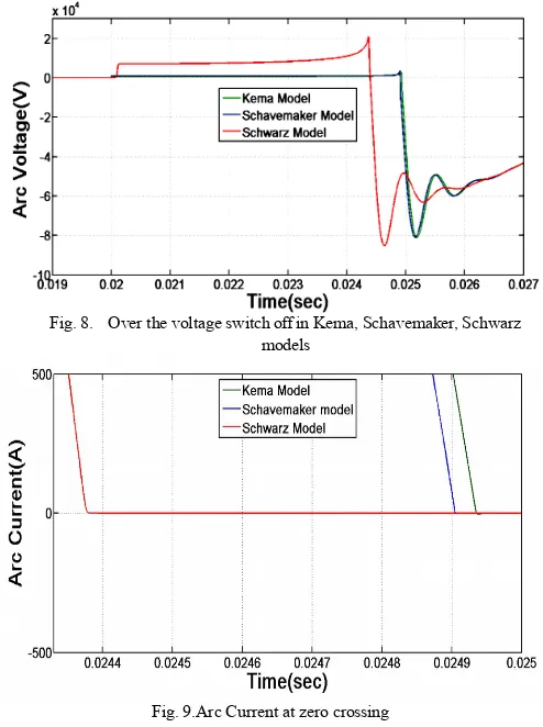
This model, a model that is modified Mayr arc time constant and power Figure 7 shows the single-phase test circuit arc models that have been studied. As the circuit in figure 7, first the current passing through the switch and voltage in three Kema, Schwarz, Schavemaker are compared, then the performance of the Schavemaker model with Genetic Algorithm Optimization and performance of the Schavemaker model with negative feedback compared.
Figure 7 test circuit disconnect switch at 0.2 s. figures 8 and 9 arc current and voltage and table 1 shows the performance of three model Kema, Schavemaker, Schwarz.
Fig. 7. Single phase test circuit
In figure 7, Vs phase angle of 90 degrees with peak amplitude of 59.196 volts and frequency is 60 Hz, and we have:
RC: R=450Ohms C=1.93 nF RL: R=29.80Ohms L=5.28mH L1=3.52mH L2=0.6256mH C=1.98μF
Fig. 8. Over the voltage switch off in Kema, Schavemaker, Schwarz models
Fig. 9.Arc Current at zero crossing
TABLE1. PERFORMANCE COMPARISON OF THREE MODELS OF KEMA,
SCHAVEMAKER, SCHWARZ IN SINGLE PHASE TEST CIRCUIT
Figures 8 and 9 and Table 1 show that Schwarz model breaks faster than two other models but voltage of breaker (switch) is higher. According to Table 1, the time to zero Schavemaker and Kema models are equal but in Figure 9, it is clear that the Schavemaker model breaks faster. So Schavemaker model for optimization is more appropriate.
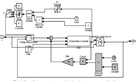
E. Schavemaker Model with Negative Feedback
Fig. 10. Schavemaker model circuit with negative feedback
Usage of this model depends on the amount of gain in this model. Changing the gain causes arc voltage and current are experiencing many changes during the breaking. Since fast opening the breaker is our optimization goal, gain variations can only reach it, but you should be very careful maximum voltage of breaker.
Arc current and voltage model Schavemaker with negative feedback with different Gain values are shown in Figures 11 and 12.
Fig. 11. Arc voltage Schavemaker model with negative feedback
Fig. 12. Arc current Schavemaker model with negative feedback
As is clear from Figure 11 and 12, gain value is greater, breaker cut off faster, but voltage goes up. The breaker design and simulation feedback should be noted that most of the breaker bearing on how much voltage. Thus, a compromise must be made. The Gain can be set between 0.1-1 and the result was good. Figures 13 and 14 show arc voltage and current at gains of 0.2 and 0.4 and 0.6. The performance comparison is shown in Table 2.
Fig. 13. Arc voltage model Schavemaker with negative feedback in 3 different Gains.
Fig. 14. Arc Current model Schavemaker with negative feedback in 3 different Gains.
TABLE2. PERFORMANCE COMPARISON OF SCHAVEMAKER MODEL WITH
NEGATIVE FEEDBACK IN 3 DIFFERENT GAINS
As Figures 13 and 14 and Table 2 show Schavemaker model with negative feedback with Gain 0.6 interrupted earlier than the rest of the state, but the maximum arc voltage is high and with Gain 0.2, arc voltage is low but it needs more time to cut off. With this interpretation, model with Gain=0.4 is closer to reality in comparison with other gain as a model for high performance simulation used in studies of high voltage circuit breaker.
VI CONCLUSION
The electric arc is an important phenomenon which determines the operation of high voltage circuit breaker. The use of modeling and simulation tools can help to improve these devices, reducing the need of prototype development and testing and so, the cost associated to this optimization process.
In this paper, the modelling of electric arc in high voltage in circuit breakers and Kema, Schwarz, Schavemaker models were studied and compared to show the superiority of the model Schavemaker, improving of break the model using the concept of negative feedback in this model. Then we see that Schavemaker model with negative feedback has the best performance compared to other models.
VII ACKNOWLEDGMENT
The authors would like to thank PSN College of
REFERENCES
[1] A. Iturregi, E. Torres, I. Zamora, “Analysis of the Electric Arc in Low Voltage Circuit Breakers,” in International Conference on Renewable Energies and Power Quality Las Palmas de Gran Canaria (Spain), 13th to 15th April, 2011.
[2] Nilesh S. Mahajan and A. A.Bhole, “Black Box Arc Modeling of High Voltage Circuit Breaker Using Matlab/Simulink,” IJEET, Volume 3, Issue 1, January- June (2012), pp. 55-63.
[3] L. Van der Sluis, “Transient in Power Systems,” John Wiley & Sons, 2001.
[4] W. 1. 0. SC 13, "State of art of circuit-breaker modeling," Cigre, Report No. 135, 1998.
[5] Pieter J, Schauemaker, Lou uan der Suis, Rent PP Smeets Vikror Kert&sz, “Digital Testing of High4oltage Circuit Breakers,” IEEE, Computer Applications in Power System.
[6] Schwarz, J. “Dynamisches Verhalten eines Gasbeblasenen, Turbulenzbestimmten Schaltlichtbogens,” ETZ-A, Bd. 92, pp. 389-391, 1971.
[7] Smeets, R.P.P., and Kertész, V. “Evaluation of High-Voltage Circuit Breaker Performance with a New Validated Arc Model,” IEE Proc.-Gener. Transm. Distrib., Vol. 147, No. 2, pp. 121-125, March 2000. [8] Parizad, A., Baghaee, H.R. Tavakoli, A., Jamali, S. “Optimization of