Hierarchically Compositional Kernels for Scalable Nonparametric Learning

(1)

Hierarchically Compositional Kernels for Scalable

Nonparametric Learning

Jie Chen [email protected]

IBM Thomas J. Watson Research Center

Haim Avron [email protected]

Tel Aviv University

Vikas Sindhwani [email protected]

Google Brain, NYC

Editor:Koji Tsuda

Abstract

We propose a novel class of kernels to alleviate the high computational cost of large-scale nonparametric learning with kernel methods. The proposed kernel is defined based on a hierarchical partitioning of the underlying data domain, where the Nystr¨om method (a globally low-rank approximation) is married with a locally lossless approximation in a hierarchical fashion. The kernel maintains (strict) positive-definiteness. The corresponding kernel matrix admits a recursively off-diagonal low-rank structure, which allows for fast linear algebra computations. Suppressing the factor of data dimension, the memory and arithmetic complexities for training a regression or a classifier are reduced from O(n2₎

andO(n3_{) to}_O₍_nr_{) and}_O₍_nr2_{), respectively, where}_n_{is the number of training examples}

andr is the rank on each level of the hierarchy. Although other randomized approximate kernels entail a similar complexity, empirical results show that the proposed kernel achieves a matching performance with a smallerr. We demonstrate comprehensive experiments to show the effective use of the proposed kernel on data sizes up to the order of millions.

Keywords: Hierarchical kernels, Nonparametric Learning

1. Introduction

Kernel methods (Sch¨olkopf and Smola, 2001; Hastie et al., 2009) constitute a principled

framework that extends linear statistical techniques to nonparametric modeling and infer-ence. Applications of kernel methods span the entire spectrum of statistical learning, in-cluding classification, regression, clustering, time-series analysis, sequence modeling (Song et al., 2013), dynamical systems (Boots et al., 2013), hypothesis testing (Harchaoui et al., 2013), and causal modeling (Zhang et al., 2011). Under a Bayesian treatment, kernel meth-ods also admit a parallel view in Gaussian processes (GP) (Rasmussen and Williams, 2006; Stein, 1999) that find broad applications in statistics and computational sciences, including

geostatistics (Chil`es and Delfiner, 2012), design of experiments (Koehler and Owen, 1996),

and uncertainty quantification (Smith, 2013).

This power and generality of kernel methods, however, are limited to moderate sized problems because of the high computational costs. The root cause of the bottleneck is the fact that kernel matrices generated by kernel functions are typically dense and

unstruc-c

(2)

tured. For n training examples, storing the matrix costs O(n2_{) memory and performing}

matrix factorizations requires O(n3_{) arithmetic operations. One remedy is to resort to}

compactly supported kernels (e.g., splines (Monaghan and Lattanzio, 1985) and Wendland functions (Wendland, 2004)) that potentially lead to a sparse matrix. In practice, however, the support of the kernel may not be sufficiently narrow for sparse linear algebra compu-tations to be competitive. Moreover, prior work (Anitescu et al., 2012) revealed a subtle drawback of compactly supported kernels in the context of parameter estimation, where the likelihood surface is bumpy and the optimum is difficult to locate. For this reason, we focus on the dense setting in this paper and the goal is to exploit structures that can reduce the prohibitive cost of dense linear algebra computations.

1.1 Preliminary

Let X be a set and let k(·,·) : X × X → _R be a symmetric and strictly positive-definite

function. Denote byX={xi ∈ X }i=1,....n a set of points. We writeK(X, X), or sometimes

K for short when the context is clear, to denote the kernel matrix of elements k(xi,xj).

Because of the confusing terminology on functions and their counterparts on matrices, here, we follow the convention that a strictly positive-definite functionkcorresponds to a positive-definite matrixK, whereas a positive-definite function corresponds to a positive semi-definite matrix. For notational convenience, we writek(x, X) to denote the row vector of elements

k(x,xj) and similarly k(X,x) to denote the column vector. In the context of

regres-sion/classification, the set X is often the d-dimensional Euclidean space Rd or a domain

S ⊂ _Rd_{. Some of the methods discussed in this paper naturally generalize to a more}

ab-stract space. Associated to each pointxi is a target valueyi∈R. We write yfor the vector

of all target values.

The Reproducing Kernel Hilbert Space H_kassociated to a kernel kis the completion of

the function space

( _m

X

i=1

αik(zi,·)|zi ∈ X, αi∈R, m∈Z+

)

equipped with the inner product

* X

i

αik(zi,·), X

j

βjk(wj,·) +

=X

ij

αiβjk(zi,wj).

Given training data {(xi, yi)}i=1,...,n, a typical kernel method finds a functionf ∈ Hk that

minimizes the following risk functional

L(f) =

n X

i=1

V(f(xi), yi) +λkfk2Hk, (1)

whereV is a loss function andλ >0 is a regularization. WhenV is the squared lossV(t, y) =

(t−y)2, the Representer Theorem (Sch¨olkopf et al., 2001) implies that the minimizer is

f(x) =k(x, X)[K(X, X) +λI]−1y, (2)

which is nothing but the well-known kernel ridge regression. Similarly, whenV is the hinge

(3)

In the GP view, the kernel k serves as a covariance function. Assuming a zero-mean

Gaussian prior with covariancek, for any separate set of pointsX∗and the associated vector

of target values y∗, the joint distribution of yand y∗ is thus

y y∗

∼ N

0,

K(X, X) K(X, X∗)

K(X∗, X) K(X∗, X∗)

.

Because of the Gaussian assumption, the posterior is the conditionaly∗|X∗, X,y∼ N(µ,Σ)

where

µ=K(X∗, X)K(X, X)−1y, (3)

and

Σ =K(X∗, X∗)−K(X∗, X)K(X, X)−1K(X, X∗). (4)

A white noise of varianceλmay be injected to the observationsyso that the mean prediction

µ in (3) is identical to (2). One may also impose a nonzero-mean model in the prior to

capture the trend in the observations (see, e.g., the classic paper O’Hagan and Kingman (1978) and also Rasmussen and Williams (2006, Section 2.7)).

Equations (2)–(4) exemplify the demand for kernels that may simplify computations

for a large K(X, X). We discuss a few popular approaches in the following. To motivate

the discussion, we consider stationary kernels whose function value depends on only the

difference of the two input arguments; that is, we can write by abuse of notationk(x,x0) =

k(r), wherer=x−x0; for example, the Gaussian kernel

k(x,x0) = exp

−kx−x 0_k2

2

2σ2

(5)

parameterized byσ. The Fourier transform ofk(r), coinedspectral density, in a sense

char-acterizes the decay of eigenvalues of the finitely dimensional covariance matrix K (Stein,

1999; Chen, 2013). The decay is known to be the fastest among the Mat´ern class of

ker-nels (Stein, 1999; Rasmussen and Williams, 2006; Chil`es and Delfiner, 2012), where Gaussian

being a special case is the smoothest. Additionally, the range parameter σ also affects the

decay. When σ → ∞,K tends to a rank-1 matrix; whereas when σ → 0, K tends to the

identity. The numerical rank of the matrix varies whenσ moves between the two extremes.

The decay of eigenvalues plays an important role on the effectiveness of the approximate kernels discussed below.

1.2 Approximate Kernels

The first approach is low-rank kernels. Examples are Nystr¨om approximation (Williams

and Seeger, 2000; Sch¨olkopf and Smola, 2001; Drineas and Mahoney, 2005), random Fourier

features (Rahimi and Recht, 2007), and variants (Yang et al., 2014). The Nystr¨om

approx-imation is based on a set of landmark points,X, randomly sampled from the training data

X. Then, the kernel can be written as

kNystr¨om(x,x0) =k(x, X)K(X, X)−1k(X,x0). (6)

For the convenience of deriving approximation bounds, Drineas and Mahoney (2005)

(4)

in (6) necessarily replaced by a pseudo inverse. Various approaches for choosing the land-mark points were compared in Zhang and Kwok (2010). For random Fourier features, let ˆ

k(ω) be the Fourier transform of k(r) and let ˆk be normalized such that it integrates to

unity; that is, ˆkis the normalized spectral density of k. Then, the kernel is

kFourier(x,x0) = 2

r

r X

i=1

cos(ω_iTx+bi) cos(ωiTx0+bi), (7)

where r is the rank, and bi and ωi are iid samples of Uniform(0,2π) and of a distribution

with density ˆk, respectively. Note that (6) applies to any kernel whereas (7) applies to only

stationary ones.

The Nystr¨om approximation admits a conditional interpretation in the context of GP.

The covariance kernel (6) can be equivalently written as

kNystr¨om(x,x0) =k(x,x0)−k(x,x0|X),

where

k(x,x0|X) =k(x,x0)−k(x, X)K(X, X)−1k(X,x0)

is nothing but the covariance ofxand x0 conditioned onX. In other words, the covariance

kernel of Nystr¨om approximation comes from a deduction of the original covariance by a

conditional covariance. The conditional covariance for any x(or symmetrically, x0) within

Xvanishes and hence the approximation is lossless. Intuitively speaking, the closer the sites

are toX, the smaller the loss is. This explains frequent observations that when the size of

the set X is small, using the centers of a k-means clustering as the landmark points often

improves the approximation (Zhang et al., 2008; Yang et al., 2012). A caveat is that the

time cost of performing k-means clustering is often much higher than that of the Nystr¨om

calculation itself. Hence, the improvement gained from clustering may not be as significant

as that from increasing the size of the conditioned setX. WhenXis large, the improvement

brought about by clustering is less significant (see, e.g., Rasmussen and Williams (2006, Section 8.3.7)).

A limitation of the low-rank kernels is that the size of the conditioned set, or equivalently

the rank, needs to correlate with the decay of the spectrum ofK in order to yield a good

approximation. For a slow decay, it is not rare to see in practice that the rankr grows to

thousands (Yen et al., 2014) or even several hundred thousands (Huang et al., 2014; Avron and Sindhwani, 2016) in order to yield comparable results with other methods, for a data set of size on the order of millions. See also the experimental results in Section 5.

The second approach is a cross-domain independent kernel. Simply speaking, the kernel matrix is approximated by keeping only the diagonal blocks of the matrix. In a GP language,

we partition the domainSintomsub-domainsSj,j = 1, . . . , m, and make an independence

assumption across sub-domains. Then, the covariance between xand x0 vanishes when the

two sites come from different sub-domains. That is,

kindependent(x,x0) = (

k(x,x0), ifx,x0 ∈Sj for somej,

0, otherwise. (8)

(5)

likelihood comparison in Stein (2014) and also the experimental results in Section 5). An intuitive explanation exists in the context of classification. The cross-domain independent kernel works well when geographically nearby points possess a majority of the signal for

classifying points within the domain. This happens more often when the kernel has a

reasonably centralized bandwidth (outside of which the kernel value becomes marginal). In such a case, nearby points are the most influential.

The third approach is covariance tapering (Furrer et al., 2006; Kaufman et al., 2008).

It amounts to defining a new kernel by multiplying the original kernel k with a compactly

supported kernelkcompact:

ktaper(x,x0) =k(x,x0)·kcompact(x,x0).

The tapered kernel matrix is an elementwise product of two positive-definite matrices; hence, it is positive-definite, too (Horn and Johnson, 1994, Theorem 5.2.1). The primary motivation of this kernel is to introduce sparsity to the matrix. The supporting theory is drawn on the confidence interval (cf. (4)) rather than on the prediction (3). It is cast in the setting of fixed-domain asymptotics, which is similar to a usual practice in machine learning—a prescaling of each attribute to within a finite interval. The theory hints that

if the spectral density of kcompact has a lighter tail (i.e., the spectrum of the corresponding

kernel matrix decays faster) than that ofk, then the ratio between the prediction variance

by using the tapered kernel ktaper and that by using the original kernelk tends to a finite

limit, as the number of training data increases to infinity in the domain. The theory

holds a guarantee on the prediction confidence if we choose kcompact judiciously. Tapering

is generally applicable to heavy-tailed kernels (e.g., Mat´ern kernels with low smoothness)

rather than light-tailed kernels such as the Gaussian. Nevertheless, a drawback of this approach is similar to the one we stated earlier for using a compactly supported kernel alone: the range of the support must be sufficiently small for sparse linear algebra to be efficient.

1.3 Proposed Kernel

In this paper, we propose a novel approach for constructing approximate kernels motivated by low-rank kernels and cross-domain independent kernels. The construction aims at deriv-ing a kernel that (a) maintains the (strict) positive-definiteness, (b) leverages the advantages of low-rank and independent approaches, (c) facilitates the evaluation of the kernel matrix

K(X, X) and the out-of-sample extension k(X,x), and (d) admits fast algorithms for a

(6)

2. Hierarchically Compositional Kernel

The low-rank kernel (in particular, the Nystr¨om approximation kNystr¨om) and the

cross-domain independent kernel kindependent are complementary to each other in the following

sense: the former acts on the global space, where the covariance at every pair of points

x and x0 are deducted by a conditional covariance based on the conditioned set X chosen

globally; whereas the latter preserves all the local information but completely ignores the interrelationship outside the local domain. We argue that an organic composition of the two will carry both advantages and alleviate the shortcomings. Further, a hierarchical composition may reduce the information loss in nearby local domains.

2.1 Composition of Low-Rank Kernel with Cross-Domain Independent Kernel

Let the domain S be partitioned into disjoint sub-domains S

Sj = S. Let X be a set of

landmark points in S. For generality, X needs not be a subset of the training data X.

Consider the function

kcompositional(x,x0) = (

k(x,x0), ifx,x0∈Sj for somej,

k(x, X)K(X, X)−1k(X,x0), otherwise.

Clearly, kcompositional leverages both (6) and (8). When two points x and x0 are located

in the same domain, they maintain the full covariance (8); whereas when they are located

in separate domains, their covariance comes from the low-rank kernel kNystr¨om (6). Such a

composition complements missing information across domains inkindependentand also

com-plements the information loss in local domains caused by the Nystr¨om approximation. The

following result is straightforward in light of the fact that ifx∈X, thenK(X, X)−1k(X,x)

is a column of the identity matrix where the only nonzero element (i.e., 1) is located with

respect to the location ofxinside X.

Proposition 1 We have

kcompositional(x,x0) =k(x,x0),

if x,x0∈Sj for some j, or if either of x,x0 belongs toX.

An alternative view of the kernel kcompositional is that it is an additive combination of

a globally low-rank approximation and local Schur complements within each sub-domain. Hence, the kernel is (strictly) positive-definite. See Lemma 2 and Theorem 3 in the following.

Lemma 2 The Schur-complement function

kSchur(x,x0) =k(x,x0)−k(x, X)K(X, X)−1k(X,x0)

is positive-definite, if kis strictly positive-definite, or if k is positive-definite andK(X, X)

is invertible.

Proof For any setX, letY =X∪X. It amounts to showing that the corresponding kernel

matrix KSchur(Y, Y) is positive semi-definite; then, KSchur(X, X) as a principal submatrix

(7)

Denote by Xc ₌ _Y_\_X_{, which could possibly be empty, and let the points in} _X _be

ordered before those inXc. Then,

KSchur(Y, Y) =

0 0

0 K(Xc_{, X}c₎₋_K₍_Xc_{, X}₎_K₍_{X, X}₎−1_K₍_{X, X}c₎

.

By the law of inertia, the matrices

K(X, X) K(X, Xc)

K(Xc_{, X}₎ _K₍_Xc_{, X}c₎

and

K(X, X) 0

0 K(Xc_{, X}c₎₋_K₍_Xc_{, X}₎_K₍_{X, X}₎−1_K₍_{X, X}c₎

have the same number of positive, zero, and negative eigenvalues, respectively. If k is

strictly positive-definite, then the eigenvalues of both matrices are all positive. If k is

positive-definite, then the eigenvalues of both matrices are all nonnegative. In both cases, the Schur-complement matrixK(Xc, Xc)−K(Xc, X)K(X, X)−1K(X, Xc) is positive semi-definite and thus so is KSchur(Y, Y).

Theorem 3 The functionkcompositionalis positive-definite ifkis positive-definite andK(X, X)

is invertible. Moreover, kcompositional is strictly positive-definite ifk is so.

Proof Write kcompositional=k1+k2, wherek1(x,x0) =k(x, X)K(X, X)−1k(X,x0) and

k2(x,x0) = (

k(x,x0)−k(x, X)K(X, X)−1k(X,x0), x,x0 ∈Sj for somej,

0, otherwise.

Clearly, k1 is positive-definite; by Lemma 2, k2 is so, too. Thus, kcompositional is

positive-definite.

We next show the strict definiteness when k is strictly positive-definite. That is, for

any set of points {xi} and any set of coefficients {αi} that are not all zero, the bilinear

form P

ilαiαlkcompositional(xi,xl) cannot be zero. Note that k2(x,x0) = 0 whenever x or

x0 ∈ X. Moreover, we have seen in the proof of Lemma 2 that the Schur-complement

matrix K(Xc, Xc)−K(Xc, X)K(X, X)−1K(X, Xc) is positive-definite when k is strictly

positive-definite. Therefore, we have P

ilαiαlk2(xi,xl) = 0 only when αi = 0 for all i

satisfying xi∈/ X. In such a case,

X

il

αiαlk1(xi,xk) = X

xi,xl∈X

αiαlk(xi, X)K(X, X)−1k(X,xl).

Because of the strict positive-definiteness of k, the above summation cannot be zero if any

of the involvedαi (that is, those satisfyingxi ∈X) is nonzero. Then,P_ilαiαl[k1(xi,xl) +

k2(xi,xl)] = 0 only when allαi are zero.

Since the composition replaces the Nystr¨om approximation in local domains by the full

covariance, it bares no surprise thatkcompositional improves overkNystr¨om in terms of matrix

(8)

Theorem 4 Given a set X of landmark points and for any set X6=X,

kK(X, X)−Kcompositional(X, X)k<kK(X, X)−KNystr¨om(X, X)k,

where k · k is the 2-norm or the Frobenius norm.

Proof Based on the splitkcompositional=k1+k2 in the proof of Theorem 3, one easily sees

that

K−Kcompositional= (K−KNystr¨om)−block-diag(K−KNystr¨om),

where block-diag means keeping only the diagonal blocks of a matrix. Denote by A =

K−KNystr¨om and D= block-diag(A). In what follows we show that

kA−Dk<kAk. (9)

Because A = K(X, X) −K(X, X)K(X, X)−1K(X, X) is positive semi-definite and

nonzero, its diagonal cannot be zero. Then, eliminating the block-diagonal part D

re-duces the Frobenius norm. Thus, (9) holds for the Frobenius norm. To see that (9) also

holds for the 2-norm, letY =X\X and let the points inY be ordered before those inX\Y.

Then,

A=

K(Y, Y)−K(Y, X)K(X, X)−1K(X, Y) 0

0 0

.

Because the zero rows and columns do not contribute to the 2-norm, and because the

top-left block of A is positive-definite, it suffices to prove (9) for any positive-definite matrix

A.

Note the following two straightforward inequalities

λmin(A−D)≥λmin(A)−λmax(D), (10) λmax(A−D)≤λmax(A)−λmin(D). (11)

BecauseDconsists of the diagonal blocks ofA, the interlacing theorem of eigenvalues states

that for each diagonal block Di, we have

λmin(A)≤λmin(Di)≤λmax(Di)≤λmax(A).

Then, taking the max/min eigenvalues of all blocks, we obtain

λmin(A)≤λmin(D)≤λmax(D)≤λmax(A). (12)

Substituting (12) into (10) and (11), together withλmin(A)>0, we obtain

λmin(A−D)>−λmax(A) and λmax(A−D)< λmax(A),

(9)

2.2 Hierarchical Composition

While kcompositional maintains the full information inside each domain Sj, the information

loss across domains caused by the low-rank approximation may still be dramatic. Consider

the scenario of a large number of disjoint domainsSj; such a scenario is necessarily typical

for the purpose of reducing the computational cost. If each domain is adjacent to only a few neighboring domains, it is possible to reduce the information loss in nearby domains.

The idea is to form a hierarchy. Let us first take a two-level hierarchy for example. A few

of the neighboring domains Sj form a super-domain SJ =Sj∈JSj. These super-domains

are formed such that they are disjoint and they collectively partition the whole domain;

i.e., S

SJ = S. Under such a hierarchical formation, instead of using landmark points X

in S to define the covariance across the bottom-level domains Sj, we may use landmark

pointsX_J chosen from the super-domainSJ to define the covariance. The intuition is that

the conditional covariance k(x,x0|X_J) forx,x0 ∈SJ tends to be smaller thank(x,x0|X),

becausex andx0 are geographically closer toX_J than toX. Then, the information loss is

reduced for points inside the same super-domainSJ.

To formalize this idea, we consider an arbitrary hierarchy, which is represented by a

rooted tree T. See Figure 1 for an example. The root node 1 is associated with the whole

domainS =:S1. Each nonleaf nodeipossesses a set of childrenCh(i); correspondingly, the

associated domain Si is partitioned into disjoint sub-domains Sj satisfying

S

j∈Ch(i) =Si.

The partitioning treeT is almost the most general rooted tree, except that no nodes in T

have exactly one child.

1

2

5 6 7

3 4

8 9

S1

S2

S3

S4

S5

S6

S7

S8

S9

Figure 1: Partitioning tree T and the domainS.

Each nonleaf node iis associated with a set X_i of landmark points, located within the

domain Si. We now recursively define the kernel on domains across levels. Continuing

the example of Figure 1, node 4 has two children 8 and 9. Since these two children are

leaf nodes, the covariance within S8 (orS9) comes from the original kernel k, whereas the

covariance across S8 and S9 comes from the Nystr¨om approximation by using landmark

points X₄. That is, the kernel is equal to k(x,x0) if x and x0 are both in S8 (or in S9),

and equal to k(x, X₄)K(X₄, X₄)−1k(X₄,x0) if they are in S8 and S9 separately. Such a

covariance bares less information loss caused by the conditioned set, compared with the use

(10)

Next, consider the covariance between child domains of S2 and those ofS4 (say,S6 and S9, respectively). At a first glance, we could have used k(x, X₁)K(X₁, X₁)−1k(X₁,x0) to

define the kernel, becauseX₁ consists of landmark points located in the domain that covers

both S6 and S9. However, such a definition cannot guarantee the positive-definiteness of

the overall kernel. Instead, we approximatek(x, X₁) by using the Nystr¨om approximation

k(x, X₂)K(X₂, X₂)−1K(X₂, X₁) based on the landmark points X₂. Then, the covariance

forx∈S6 and x0 ∈S9 is defined as

h

k(x, X₂)K(X₂, X₂)−1K(X₂, X₁)iK(X₁, X₁)−1hK(X₂, X₁)K(X₂, X₂)−1k(X₂,x0)i.

Formally, for a leaf node j and x,x0 ∈ Sj, define k(j)(x,x0) ≡k(x,x0). For a nonleaf

node iandx,x0 ∈Si, define

k(i)(x,x0) := (

k(j)_(x_,_x0₎_, _if_x_,_x0 _∈_S

j for somej∈Ch(i),

ψ(i)_(x_{, X}

i)K(Xi, Xi)−1ψ(i)(Xi,x0), otherwise,

(13)

where ifj is a child of iand if x∈Sj, then

ψ(i)(x, X_i) := (

k(x, X_i), ifj is a leaf node,

ψ(j)_(x_{, X}

j)K(Xj, Xj)−1K(Xj, Xi), otherwise.

(14)

The k(i) _{at the root level gives the} _{hierarchically compositional kernel} _{of this paper:}

khierarchical:=k(root). (15)

Clearly, the kernel kcompositional in Section 2.1 is a special case of khierarchical when the

partitioning tree consists of only the root and the leaf nodes (which are children of the root).

Expanding the recursive formulas (13) and (14), for two distinct leaf nodes j and l, we

see that the covariance betweenx∈Sj and x0 ∈Sl is

khierarchical(x,x0) =k(r)(x,x0)

=k(x, X_j₁)K(X_j₁, X_j₁)−1K(X_j₁, X_j₂)· · ·K(X_j_s, X_j_s)−1K(X_j_s, X_r)

| {z }

ψ(r)_(x_,X r)

K(X_r, X_r)−1

·K(X_r, X_l_t)K(X_l_t, X_l_t)−1· · ·K(X_l₂, X_l₁)K(X_l₁, X_l₁)−1k(X_l₁,x0)

| {z }

ψ(r)₍_X r,x0)

, (16)

whereris the least common ancestor ofjandl, and (j, j1, j2, . . . , js, r) and (l, l1, l2, . . . , lt, r)

are the paths connecting r and the two leaf nodes, respectively. Therefore, we have the

following result.

Proposition 5 Based on the notation in the preceding paragraph, for x∈Sj and x0 ∈Sl,

we have

khierarchical(x,x0) =k(x,x0),

(11)

Proof On (16), recursively apply the fact that ifx∈X, thenK(X, X)−1k(X,x) is a col-umn of the identity matrix where the only nonzero element (i.e., 1) is located with respect

to the location ofxinside X.

The following theorem guarantees the validity of the kernel. Its proof strategy is similar

to that of Theorem 3, but it is complex because of recursion. We defer the proof to

Appendix A.

Theorem 6 The functionkhierarchicalis positive-definite ifkis positive-definite andK(Xi, Xi)

is invertible for all sets of landmark pointsX_iassociated with the nonleaf nodesi. Moreover, khierarchical is strictly positive-definite if kis so.

3. Matrix View

The kernel matrix Khierarchical(X, X) for a set of training points X exhibits a hierarchical

block structure. Figure 2 pictorially shows such a structure for the example in Figure 1.

To avoid degenerate empty blocks, we assume that X∩Sj 6=∅ for all leaf nodes j in the

partitioning tree T.

A55 A56 A57

A65 A66 A67

A75 A76 A77

A88 A89

A98 A99

A23 A24

A32 A33 A34

A42 A43

Figure 2: The matrix Khierarchical corresponding to the partitioning treeT in Figure 1.

Formally, for any node i, letXi =X∩Si; that is,Xi consists of the training points that

fall within the domainSi. Then, define a matrixA∈Rn×n with the following structure:

1. For every nodei,Aiiis a diagonal block whose rows and columns correspond toXi; for

every pair of sibling nodesiandj,Aij is an off-diagonal block whose rows correspond

toXi and columns to Xj.

2. For every leaf nodei,Aii=K(Xi, Xi).

3. For every pair of sibling nodesiandj,Aij =UiΣpUjT, wherep is the parent ofiand

(12)

4. For every nonleaf node p, Σp =K(Xp, Xp).

5. For every leaf nodei,Ui =K(Xi, Xp)K(Xp, Xp)−1, wherep is the parent of i.

6. For every pair of child node iand parent node p not being the root, the block of Up

corresponding to node i is UiWp, where Wp =K(Xp, Xr)K(Xr, Xr)−1 and r is the

parent ofp. That is, in the matrix form,

Up= 

   .. .

Ui

.. .



  

i∈Ch(p) ·Wp.

One sees thatA is exactly equal to Khierarchical(X, X) by verifying against the definition of

khierarchical in (13)–(15).

Such a hierarchical block structure is a special case of the recursively low-rank

com-pressed matrix studied in Chen (2014b). In this matrix, off-diagonal blocks are recursively compressed into low rank through change of basis, while the main-diagonal blocks at the leaf level remain intact. Its connections and distinctions with related matrices (e.g., FMM matrices (Sun and Pitsianis, 2001) and hierarchical matrices (Hackbusch, 1999)) were dis-cussed in detail in Chen (2014b). The signature of a recursively low-rank compressed matrix is that many matrix operations can be performed with a cost, loosely speaking, linear in

n. The matrix structure in this paper, which results from the kernelkhierarchical, specializes

a general recursively low-rank compressed matrix in the following aspects: (a) the matrix

is symmetric; (b) the middle factor Σp in each Aij is the same for all child pairs i, j of p;

and (c) the change-of-basis factor Wp is the same for all children i of p. Hence, storage

and time costs of matrix operations are reduced by a constant factor compared with those of the algorithms in Chen (2014b). In what follows, we discuss the algorithmic aspects of the matrix operations needed to carry out kernel method computations, but defer the complexity analysis in Section 4. Discussions of additional matrix operations useful in a general machine learning context are made toward the end of the paper.

3.1 Matrix-Vector Multiplication

First, we consider computing the matrix-vector producty=Ab. Let the blocks of a vector

be labeled in the same manner as those of the matrix A. That is, for any node i, bi

denotes the part ofbthat corresponds to the point set Xi. Then, the vectory is clearly an

accumulation of the smaller matrix-vector products Aijbj in the appropriate blocks, for all

sibling pairs i, j and for all leaf nodes i=j (cf. Figure 2). When i=j is a leaf node, the

computation ofAijbj is straightforward. On the other hand, wheniandj constitute a pair

of sibling nodes, we consider a descendant leaf nodelofi. The block ofAijbj corresponding

to node ladmits an expanded expression

UlWl1Wl2· · ·WlsWiΣpW T j



 X

qt∈Ch(j)

W_qT_t· · ·



 X

q2∈Ch(q3)

W_qT₂



 X

q1∈Ch(q2)

W_qT₁



 X

q∈Ch(q1)

U_qTbq 

 

,

(13)

where (l, l1, l2, . . . , ls, i, p) is the path connecting l and the parent p of i. This expression

assumes that all the leaf descendants of j are on the same level so that the expression is

not overly complex; but the subsequent reasoning applies to the general case. The terms inside the nested parentheses of (17) motivate the following recursive definition:

ci = 

 

 

U_iTbi, iis a leaf node,

W_iT X

j∈Ch(i)

cj, otherwise.

Clearly, all cj’s can be computed within one pass of a post-order tree traversal. Upon the

completion of the traversal, we rewrite (17) asUlWl1Wl2· · ·WlsWiΣpcj. Then we note that

for any leaf nodel,yl is a sum of these expressions with allp along the path connecting l

and the root, and additionally, of Allbl. In other words, we have

yl=Allbl+ 



X

l0_∈_Ch₍_l 1)\{l}

UlΣl1cl0 

+





X

l0_∈_Ch₍_l 2)\{l1}

UlWl1Σl2cl0   +· · ·+   X

l0_∈_Ch_(root)\{_l t}

UlWl1Wl2· · ·WltΣrootcl0 

,

where (l, l1, l2, . . . , lt,root) is the path connecting l and the root. Therefore, we recursively

define another quantity

dj =Widi+

X

j0_∈_Ch₍_i_)\{_j_} Σicj0

for all nonroot nodes j with parent i. Clearly, all dj’s can also be computed within one

pass of a pre-order tree traversal. Upon the completion of this second traversal, we have

yl=Allbl+Uldl, which concludes the computation of the whole vector y.

As such, computing the matrix-vector product y =Ab consists of one post-order tree

traversal, followed by a pre-order one. We refer the reader to Chen (2014b) for a full account of the computational steps. For completeness, we summarize the pesudocode in Algorithm 1 as a reference for computer implementation.

3.2 Matrix Inversion

Next, we consider computing A−1, for which we use the tilded notation ˜A := A−1. One

can show (Chen, 2014b) that ˜A has exactly the same hierarchical block structure as does

A. In other words, the structure of ˜A can be described by reusing the verbatim at the

beginning of Section 3, with the factors Aii,Aij,Ui, Σp,Wp replaced by the tilded version

˜

Aii, ˜Aij, ˜Ui, ˜Σp, ˜Wp, respectively. The proof is both inductive and constructive, providing

explicit formulas to compute ˜Aii, ˜Aij, ˜Ui, ˜Σp, ˜Wp level by level. The essential idea is that if

(Aii−UiΣpU_iT)−1= ˜Aii−U˜iΣ˜pU˜_iT have been computed for all children iof a nodep, and

ifr is the parent of p, then

App−UpΣrUpT = 

  

. ..

Aii−UiΣpU_iT

. ..     +     .. . Ui .. .     Σp

· · · UT i · · ·

(14)

Algorithm 1 Computingy=Ab

1: Initialize ci←0,di←0 for each nonroot node iof the tree

2: _Upward(root)

3: _Downward(root)

4: function Upward(i)

5: if iis leaf then

6: ci ←UiTbi; yi ←Aiibi

7: else

8: for allchildrenj ofido

9: Upward(j)

10: ci←ci+WiTcj,if iis not root

11: end for

12: end if

13: if iis not rootthen

14: for allsiblings lof idodl←dl+ Σpci end for . pis parent ofi 15: end if

16: end function

17: function Downward(i)

18: if iis leaf thenyi ←yi+Uidi and return end if

19: for all childrenj of ido

20: d_j ←d_j+Widi,if iis not root

21: _Downward(j)

22: end for

23: end function

Hence, the inversion of App−UpΣrUpT can be done by applying the Sherman–Morrison–

Woodbury formula, which results in a form ˜App−U˜pΣ˜rU˜pT, where ˜Wr is determined based

on the change of basis from ˜Ui to ˜Up and the middle factor ˜Σr is also determined. In

ad-dition, the factors ˜Σj (computed previously) for all descendants j of r must be corrected

because the diagonal block of ˜App corresponding to node j is a low-rank correction of the

corresponding diagonal block of ˜Aiiwith the same basis. Such a down-cascading correction

occurs whenever the induction proceeds from one child level to the parent level; but com-putationally, the correction on any node can be accumulated during the whole induction

process. The net result of the accumulation is that each ˜Σi needs be corrected only once,

which ensures an efficient computation.

(15)

Algorithm 2 Computing ˜A=A−1

1: _Upward(root)

2: _Downward(root)

3: function Upward(i)

4: if iis leaf then

5: A˜_ii←(Aii−UiΣpUiT)

−1_; _U_˜

i←A˜iiUi; Θ˜i←UiTU˜i . pis parent ofi

6: return

7: end if

9: _Upward(j)

10: W˜j ←(I+ ˜ΣjΞ˜j)Wj if j is not leaf

11: Θ˜j ←WjTΞ˜jW˜j if j is not leaf

12: end for

13: Ξ˜i ←P_j∈Ch(i)Θ˜j

14: if iis not rootthen Λ˜i ←Σi−WiΣpWiT elseΛ˜i←Σi end if . pis parent ofi

15: Σ˜i ← −(I+ ˜ΛiΞ˜i)−1Λ˜i

17: E˜_j ←W˜_jΣ˜iW˜jT if j is not leaf 18: end for

19: E˜_i ←0 if iis root

20: end function

21: function Downward(i)

22: if iis leaf then

23: A˜ii←A˜ii+ ˜UiΣ˜pU˜iT ifiis not root . pis parent ofi

24: else

25: E˜i ←E˜i+ ˜WiE˜pW˜iT ifiis not root . pis parent ofi

26: Σ˜i←Σ˜i+ ˜Ei

27: for allchildrenj ofido Downward(j) end for 28: end if

29: end function

3.3 (Implicit) Out-of-Sample Construction

Now, we consider the vectorkhierarchical(X,x) for an existing training setX and a new point

x in the testing set. Generally, this vector is not used alone but it appears in the inner

product with some other vectorw (see (2)). Whereas the construction ofkhierarchical(X,x)

can be done atO(n) cost (details omitted here), we shall consider instead the computation

of the inner productwT_{khierarchical}₍_X,_{x), because the cost of computing this inner product}

(16)

preprocessing cost is amortized on eachxand thus is generally negligible for a large number

of x’s.

The computation ofwT_k

hierarchical(X,x) was not described in Chen (2014b), but the idea

is similar to that of the matrix-vector multiplication in Section 3.1. To simplify notation, letv≡khierarchical(X,x). Assume thatxfalls in the domainSj for some leaf nodej. Then,

vj =k(Xj,x) and for any leaf nodel6=j,

vl =UlWl1Wl2· · ·WlsΣpW T jt · · ·W

T j2W

T

j1K(Xj1, Xj1)

−1_k₍_X

j1,x),

wherepis the least common ancestor oflandj, and (l, l1, l2, . . . , ls, p) and (j, j1, j2, . . . , jt, p)

are the paths connectingl andp, andj andp, respectively. Therefore, if we define

dju =W T

judju−1, · · · dj2 =W T

j2dj1, dj1 =W T

j1dj, dj =K(Xj1, Xj1)

−1_k₍_X

j1,x), (18) where (j, j1, j2, . . . , ju,root) is the path connectingj and the root, then we have

wTv=w_jTk(Xj,x) + X

l6=j, lis leaf

wT_l UlWl1Wl2· · ·WlsΣpdjt. (19)

If we further define

el= 

 

 

U_lTwl, l is leaf,

X

i∈Ch(l) WT

l ei, otherwise, and cq = Σ

T

pel, (20)

wherep is the parent of the sibling pairq and l, then (19) is simplified to

wTv=wT_jk(Xj,x) +

X

jt∈path(j,root)

cT_j_tdjt. (21)

Based on (18)–(21), we see that wT_v _≡ _wT_k

hierarchical(X,x) can be computed in the

following two phases. In the first phase, we compute el and cl for all nonleaf nodes l

according to (20). Such a computation can be done by using a post-order tree traversal

and is independent of x. Thus, this computation is the preprocessing step. In the second

phase, we compute djt for all jt along the path (j, j1, j2, . . . , ju,root) according to (18). Once they are computed, the summation (21) is straightforward and we thus conclude the computation. Note that the second phase is always conducted along a certain path

connecting the root and the leaf j. As long as the determination of which leaf j the point

x falls in is restricted on this path, the cost of the second phase is always asymptotically

smaller than that of a tree traversal. We summarize the pseudocode in Algorithm 3.

4. Practical Considerations

Sections 2 and 3 provide a general framework for the interpretation of and the computation

with the proposed kernel khierarchical; they, however, have not covered a range of practical

(17)

Algorithm 3 Computingz=wT_k

hierarchical(X,x) for x∈/ X

1: Prefactorize K(X_p, X_p) for all parents pof leaf nodes

2: Initialize ci←0,di←0 for each nonroot node iof the tree

3: _{Common-Upward}(root)

. The above three steps are independent of x and are treated as precomputation. In

computer implementation, the intermediate resultsci are carried over to the next step

Second-Upward, whereas the contents of di are discarded and the allocated memory

is reused.

4: _{Second-Upward}(root)

5: function Common-Upward(i)

6: if iis leaf then

7: di ←UiTwi

8: else

9: for allchildrenj ofido

10: _{Common-Upward}(j)

11: d_i ←d_i+WT

i dj,if iis not root 12: end for

13: end if

14: if iis not rootthen

15: for allsiblings lof idocl ←ΣTpdi end for . pis parent ofi 16: end if

17: end function

18: function Second-Upward(i)

19: if iis leaf then

20: d_i ←K(X_p, X_p)−1k(X_p,x) . pis parent ofi

21: z←w_iTk(Xi,x)

22: else

23: Find the childj (among all children ofi) wherexlies on

24: _{Second-Upward}(j)

25: di ←WiTdj ifiis not root

26: end if

27: z←z+cT

idi ifiis not root 28: end function

4.1 Partitioning of Domain

Whereas the partitioning of a low-dimensional domain can be made regular, the partitioning of a high-dimensional domain is inherently difficult because of the curse of dimensionality. Several data-driven approaches appear to be natural choices but they have pros and cons.

(18)

the case that some attributes of the data are binary and the counts are highly imbalanced. These attributes sometimes result from a conversion of categorical attributes to numeric ones. Partitioning on these axes is unlikely to be balanced. An alternative is to partition the axis into two segments of equal length. This approach often results in highly imbalanced partitioning because data are generally not evenly distributed.

The k-means (MacQueen, 1967) approach partitions a point set through a k-means clustering and hence the partitioning is a Voronoi diagram of the cluster centers. The resulting tree is not necessarily binary if there exhibits more than two natural clusters in the data on some level. An advantage of this approach is that the clustering often results

in a tight grouping of the points, such that the subsequent Nystr¨om approximations bare

a good quality. A disadvantage is that the approach suffers from loss of clusters during iterations and it is less robust if only one set of initial guesses is used. Our experience indicates that a robust implementation of k-means sometimes costs much more than does the rest of the training computation.

The PCA (Pearson, 1901) approach recursively partitions the data according to the prin-cipal axis (the direction along which the data varies the most). This approach is based on a Gaussian assumption and often results in compact partitions if the data indeed conforms to this assumption. However, it ignores the skewness and other higher order moments, which are also crucial to the shape of data in high dimensions. In the standard case, the hyperplane that partitions the data passes through the mean, which may result in highly imbalanced partitions. An alternative is to move the hyperplane along the principal di-rection such that the two partitions are always balanced. Computationwise, this approach requires computing the dominant singular vectors of the shifted data matrix (Chen et al., 2009), which can be achieved by using a power iteration (Golub and Van Loan, 1996) or the Lanczos algorithm (Saad, 2003). However, even if we compute the singular vectors only approximately, we find that the cost is still too high (see e.g., Section 5.2).

For computational efficiency, we recommend the random projection (Johnson and Lin-denstrauss, 1984) approach. This approach uses a random vector as the normal direction of the partitioning hyperplane and positions the hyperplane such that the numbers of points on the two sides are balanced. Computationwise, it amounts to projecting the points along the random direction and splitting them in two halves around the median. This approach is motivated by the study of dimension reduction, where it was observed that the projection quality on a random subspace is as good as that on the space spanned by the dominant singular vectors, in the sense that Euclidean distances are approximately preserved (Das-gupta and Gupta, 2002). Moreover, the heuristic use of a one-dimensional subspace for projection is robust and is computationally highly efficient. In such a case, the purpose is not to preserve the Euclidean distance, but rather, to serve as an efficient procedure for partitioning. In our experience, the eventual regression/classification performance of using this approach is almost identical to that of the PCA approach (see Section 5.2).

Under random projection, one can quickly determine which partition a new pointxlies

(19)

4.2 Choice of Landmark Points

The set of landmark points X_i associated to each domain Si simply consists of uniformly

random samples of the point setXi.

Some alternatives exist. Using the k-means centers of Xi as the landmark points may

improve the Nystr¨om approximations, but computing them for every nonleaf node i is

often much more expensive than the rest of the training computation. On the other hand,

using the uniformly random samples of the domain Si as the landmark points may sound

theoretically preferable, but they are difficult to compute because the domains are polyhedra rather than regular shapes (e.g., boxes).

We mentioned in Section 2.2 that the compositional kernelkcompositionalis a special case

ofkhierarchical, if in the partitioning tree every child of the root is a leaf node. Interestingly,

another interpretation exists. If we relax the requirement that the landmark pointsX_imust

reside within the domainSi, then for any partitioning tree, using the same set of landmark

pointsX_i for everyialso results in the compositional kernelkcompositional. By following the

proof of Theorem 6, one sees that the relation X_i ⊂Si is in fact nonessential. Hence, the

requirementX_i ⊂Si reflects only the modeling desire of a better kernel approximation in

local domains; it is not a necessary condition for kernel validity.

4.3 Numerical Stability

A notorious numerical challenge for kernel matrices K is that they are exceedingly

ill-conditioned as the size increases. Hence, the regularization λI serves as an important

rescue of matrix inversion. This challenge is less severe for the matrix of the proposed

kernel, Khierarchical(X, X), but since the components of this matrix are defined with the

term K(X_i, X_i)−1 for nonleaf nodes i, one must ensure that each K(X_i, X_i) is not too

ill conditioned. Generally, when the set X_i is not large, the conditioning of K(X_i, X_i)

is acceptable; however, for a robust safeguard, we use a small λ0 _{< λ} _{for help. Instead}

of treating k(x,x0) as the base kernel and λ as the amount of regularization, we treat

k0(x,x0) = k(x,x0) +λ0δx,x0 as the base kernel and λ−λ0 the regularization, where δ is

the Kronecker delta. Then, we use k0 _{to build the kernel}_k0

hierarchical and add to the matrix K_hierarchical0 a regularization (λ−λ0)I.

4.4 Sizes

Two parameters exist for the proposed kernel. First, the recursive partitioning needs a stopping criterion; we say that a set of points is not further partitioned when the cardinality

is less than or equal ton0. Second, we need to specify the sizes of the conditioned sets X_i.

Whereas one may argue that the conditioned set needs to grow with the size of the point set

for maintaining the approximation quality, a substantial increase in the size of X_i across

levels will result in too high a computational cost, forfeiting the purpose of the kernel.

Therefore, we mandate that each conditioned set have the same sizer.

It will be convenient if we can consolidate the two parameters so that different approx-imate kernels are comparable. It will also be beneficial to have a guided choice of them.

These requirements are indeed achievable. Under a balanced binary partitioning, n0 can

(20)

is not sensible to have the rank r greater than n0 because the smallest off-diagonal blocks

have a size at mostn0×n0. Then, we take

n0 =dn/2je and r =bn/2jc for somej. (22)

4.5 Cost Analysis

We are now ready to perform a full analysis of the computational costs based on the practical choices made in the preceding subsections.

Memory Cost Let us first consider the memory cost of storing the matrixA. For

simi-plicity, assume that n is a power of 2 (and thus n0 = r). Then, the partitioning tree has

n/n0 leaf nodes and n/n0−1 nonleaf nodes. Hence, the memory costs for the factors Aii,

Ui, Σp, and Wp are n20n/n0, nr, r2(n/n0−1), and r2(n/n0−1), respectively. Therefore,

the total memory cost is approximately 4nr.

Arithmetic Cost, Algorithm 1 The arithmetic cost of matrix-vector multiplication

(Algorithm 1) isO(nr), because the subroutines Upward and Downwardfor each node

performs O(r2_{) calculations, discounting the recursion calls. These recursions essentially}

constitute a tree traversal, which visits all the 2n/n0−1 nodes. Therefore, the total cost is

O(nr). In fact, a more detailed analysis may reveal the constant inside the big-O notation.

Note that the matrix-vector multiplications WT

i cj and Widi occur for each node j, Σpci

occurs for each nodei, andUT

i bi,Aiibi, andUidi occur for each leaf nodei. The matrix size

of all these multiplications isr×r. Therefore, if each multiplication requires 2r2 _arithmetic

operations, then the total cost is approximately 2r2_×₍₂_n/n

0 + 2n/n0+ 2n/n0+n/n0+

n/n0+n/n0) = 18nr, ignoring lower-order terms.

Arithmetic Cost, Algorithm 2 Based on a similar argument, the arithmetic cost of

matrix inversion (Algorithm 2) isO(nr2_{). A more precise estimate is 37}_nr2_{, if factorizing a}

general r×r matrix, factorizing a symmetric positive-definite matrix, performing a

trian-gular solve, and multiplying twor×rmatrices require 2r3_/_3,_r3_/_3,_r2_{, and 2}_r3 _operations,

respectively. As before, we ignore the lower-order terms.

Arithmetic Cost, Algorithm 3, Precomputation Phase Now consider the

precom-putation phase of the inner product wT_{khierarchical}₍_X,_{x) (Algorithm 3). In computer}

im-plementation, we move the first line (prefactorizingK(X_p, X_p)) to the matrix construction

part (to be discussed in Section 4.5). Hence, the precomputation of Algorithm 3 is

domi-nated by the third line Common-Upward(root). The arithmetic cost is O(nr), or 10nr

in a more precise account.

Arithmetic Cost, Algorithm 3, x-Dependent Phase Assume that evaluating the

kernel function k(x,x0) requires O(nz(x) + nz(x0)) arithmetic operations, where nz(·)

de-notes the number of nonzeros of a data point. Further assume that for two point setsY and

Zof sizesnY andnZrespectively, evaluating the vectork(Y,x) requiresO(nY nz(x)+nz(Y))

operations, and evaluating the matrixK(Y, Z) requiresO(nY nz(Z) +nZnz(Y)) operations,

where the notation nz(·) is extended for point sets in a straightforward manner.

Now we consider the cost of the x-dependent phase of Algorithm 3. Line 20 costs

O(rnz(x) + nz(X_p)) +O(r2_{), where the first term comes from evaluating}_k₍_X

(21)

second term a linear-solve. Note that the matrix K(X_p, X_p) has already been evaluated and prefactorized prior to this phase. In fact, such a computation is done when constructing

Khierarchical. Similarly, line 21 costsO(n0nz(x) + nz(Xi)) +O(n0). Line 23 costsO(nz(x)),

because it amounts to projectingxon a direction. Then, the overall cost of thex-dependent

phase of Algorithm 3 is

Ornz(x) + nz(Xi) + nz(Xp) + (r2+ nz(x)) log2(n/r)

, (23)

wherex lies in the leaf nodeiand p is its parent.

Arithmetic Cost, Matrix Construction We shall also consider the cost of

hierarchi-cal partitioning and the instantiation of the matrix A = Khierarchical. In the partitioning

of a set of n points X, generating a random projection direction costs O(d), computing

the projected coordinates costs O(nz(X)), finding the median costs O(n), and

permut-ing the points costs O(nz(X)). Then, counting recursion, the total cost is O((d+n+

nz(X)) log₂(n/r)). On the other hand, in the instantiation of the matrixA, computingAii

for all leaf nodesicostsO(rnz(X)), computingUi for all leaf nodesicostsO(r[n+ nz(X) + P

iis leafnz(Xp)]), computing Σpfor all nonleaf nodespcostsO(r[Ppis nonleafnz(Xp)]),

fac-torizing these Σp’s costs O(nr2), computing Wi for all nonleaf and nonroot nodes i costs

O(r[n+P

iis not leaf and not rootnz(Xi) + nz(Xp)]), and finding all landmark point sets costs

O(n). Therefore, the total cost of instantiatingAisO(r[nr+ nz(X) +P

iis not leafnz(Xi)]).

Arithmetic Cost Summary, Training and Testing Summarizing the above analysis,

we see that the overall cost of training (including partitioning, instantiating A, matrix

inversion, matrix-vector multiplication, and preprocessing of Algorithm 3) is

O (d+n+ nz(X)) log₂(n/r) +nr2+r

"

nz(X) + X

iis not leaf

nz(X_i) #!

. (24)

The overall cost of testing per xhas been given in (23).

We remark that the term log₂(n/r) in both (23) and (24) is dominated by r when n≤

r2r. Moreover, when the data X is dense, the training cost (24) simplifies toO(nr2₊_ndr₎

and the testing cost per point (23) simplifies toO(r3₊_dr_{). Suppressing the data dimension}

d, these costs are further simplified toO(nr2_{) and}_O₍_r3_{), respectively.} 5. Experimental Results

(22)

Table 1: Data sets.

Name Type d nTrain n0 _Test

cadata regression 8 16,512 4,128

YearPredictionMSD regression 90 463,518 51,630

ijcnn1 binary classification 22 35,000 91,701

covtype.binary binary classification 54 464,809 116,203

SUSY binary classification 18 4,000,000 1,000,000

mnist 10 classes 780 60,000 10,000

acoustic 3 classes 50 78,823 19,705

covtype 7 classes 54 464,809 116,203

Table 1 summarizes the data sets used for experiments. They were all downloaded from_{http://www.csie.ntu.edu.tw/~cjlin/libsvm/} and are widely used as benchmarks of kernel methods. We selected these data sets primarily because of their varying sizes. Some of the data sets come with a training and a testing part; for those not, we performed a 4:1 split to create the two parts, respectively. In some of the data sets, the attributes

had already been normalized to within [0,1] or [−1,1]; for those not, we performed such a

normalization. We also preprocessed the data sets by removing duplicate and conflicting records (whose labels are inconsistent) in the training sets. Such records are infrequent.

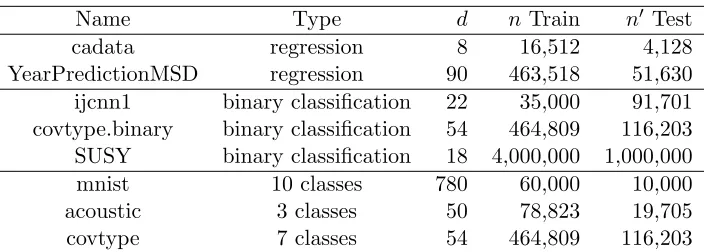
5.1 Effect of Randomness

Throughout Section 5, we will compare various approximate kernels: Nystr¨om

approxima-tionkNystr¨om, random Fourier featureskFourier, cross-domain independent kernelkindependent,

and the proposed kernelkhierarchical. The partitioning in the cross-domain independent

ker-nel is the same as that in the proposed kerker-nel, except that the hierarchy is flattened. Because of the random nature of all these kernels (e.g., landmark points, sampling, and partitioning),

we first study how the performance is affected by randomization. Note that the quantityr

is comparable across kernels, even though its specific meaning is different.

The data set for demonstration is cadata. We use the Gaussian kernel (5) as an example.

As hinted earlier, the choice of the range parameterσ affects the quality of various kernels.

Therefore, the experiment setup is to use a reasonable regularization λ= 0.01 and to vary

the choice of σ in a large interval (between 0.01 and 100) such that the optimal σ falls

within the interval. We set the rank r (and the leaf size n0) according to (22) with three

particular choices: r= 32, 129, and 516.

For each r, we repeat 30 times with different random seeds; but the seed always stays

the same every time when the range ofσis swept. The results (relative testing error versus

σ) are summarized in Figure 3, with mean (blue curve) and standard deviation (red band)

plotted. One sees that the red bands of random Fourier features are not smooth; this is because each single error curve from a fixed seed is nonsmooth. Moreover, the error

curves for Nystr¨om approximation have a nonnegligible variation when σ is small, whereas

those for the independent kernel vary significantly when σ is large. The error curves of the

(23)

σ

10-2 10-1 100 101 102

Relative error

0.2 0.3 0.4 0.5

Nystrom, r = 32

σ

10-2 10-1 100 101 102

Relative error

0.2 0.3 0.4 0.5

Nystrom, r = 129

σ

10-2 10-1 100 101 102

Relative error

0.2 0.3 0.4 0.5

Nystrom, r = 516

(a) Nystr¨om approximation

σ

10-2 10-1 100 101 102

Relative error

0.2 0.3 0.4 0.5

Fourier, r = 32

σ

10-2 10-1 100 101 102

Relative error

0.2 0.3 0.4 0.5

Fourier, r = 129

σ

10-2 10-1 100 101 102

Relative error

0.2 0.3 0.4 0.5

Fourier, r = 516

(b) random Fourier features

σ

10-2 10-1 100 101 102

Relative error

0.2 0.3 0.4 0.5

Independent, r = 32

σ

10-2 10-1 100 101 102

Relative error

0.2 0.3 0.4 0.5

σ

10-2 10-1 100 101 102

Relative error

0.2 0.3 0.4 0.5

(c) Cross-domain independent kernel

σ

10-2 10-1 100 101 102

Relative error

0.2 0.3 0.4 0.5

Hierarchical, r = 32

σ

10-2 10-1 100 101 102

Relative error

0.2 0.3 0.4 0.5

σ

10-2 10-1 100 101 102

Relative error

0.2 0.3 0.4 0.5

(d) Hierarchically compositional kernel

Figure 3: Regression error curves versusσ. Results are summarized from 30 repeated runs

(24)

speaking, asr increases, all approximate kernels yield a more and more stable error curve,

except the peculiar case of the independent kernel at largeσ.

The unstable performance caused by randomness is unfavorable for parameter estima-tion, because the valley, where the optimal parameter stands, may move substantially. The nonsmoothness exhibited in the Fourier approach also renders difficulty. Although the

un-favorable behaviors are substantially alleviated when r increases to 516 in this particular

data set, to our experience, the relieving size forr correlates with the data size; that is, the

larger n, the higher r needs to increase to. In this regard, the proposed kernel is the most

favorable because its performance is relatively stable even for small r.

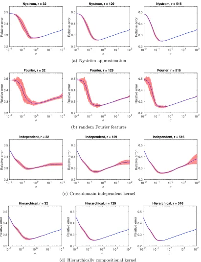
5.2 Partitioning Approaches

We further compare the methods for partitioning needed by the proposed kernel. The comparison focuses on three aspects: effect of randomness, testing error, and computa-tional efficiency. Among the several possible choices discussed in Section 4.1, only the PCA approach and the random projection approach (which is recommended) yield a balanced partitioning; hence, we compare only these two.

σ

10-2 10-1 100 101 102

Relative error

0.2 0.3 0.4 0.5

σ

10-2 10-1 100 101 102

Relative error

0.2 0.3 0.4 0.5

σ

10-2 10-1 100 101 102

Relative error

0.2 0.3 0.4 0.5

(a) Random partitioning

σ

10-2 10-1 100 101 102

Relative error

0.2 0.3 0.4 0.5

Hierarchical (PCA), r = 32

σ

10-2 10-1 100 101 102

Relative error

0.2 0.3 0.4 0.5

σ

10-2 10-1 100 101 102

Relative error

0.2 0.3 0.4 0.5

(b) PCA partitioning

Figure 4: Regression error curves of the proposed method. Data are recursively partitioned by using random projections (top row) and by PCA (bottom row), respectively.

(25)

the mean error curves are almost identical in both approaches. PCA is less influenced by randomization. Such a result should not be surprising, because PCA bares no randomness at all on partitioning; the only randomness comes from the landmark points. Although the variation of the error curves of the random projection approach is higher, such a variation is acceptable, particularly when it is compared with that of other approximate kernels in the preceding subsection.

The essential reason why random projection is favored over PCA comes from the con-sideration of computational efficiency. To generate the normal direction of a partitioning

hyperplane, random projection amounts to only generating d random numbers, whereas

PCA requires computing the dominant singular vector of the shifted data matrix. Table 2 presents the time costs of the additional singular vector computation, against the parti-tioning cost and the overall training cost by using random projection. We call the singular vector computation “overhead.” The overhead is much higher with respect to the parti-tioning step, because such a step has a negligible cost compared to the overall training.

The overhead is also generally higher whenr is smaller because there requires more

parti-tioning. The overhead with respect to partitioning easily exceeds 100% for quite a few of the data sets, and sometimes it is even a few thousand percents. For the data set mnist,

which has the largest dimensiond, the overhead with respect to overall training ranges from

approximately 50% to 800%.

5.3 Performance Results for Various Data Sets

We now compare various approximate kernels on all the data sets listed in Table 1. For each

kernel and each r, we obtain the performance result through a grid search of the optimal

parameters σ and λ. Because of the high cost of parameter tuning, no repetitions are run

and hence the performances may be susceptible to randomization. Hence, conclusions are drawn across data sets and we refrain from over-interpreting the results of an individual

data set. We run experiments with a few r’s and we are particularly interested in the

performance trend as r increases.

The results are summarized in Figures 5 and 6. In the panel of the plots, each row

corresponds to one data set. The three columns are performance versus r, training time,

and memory consumption, respectively. The performance is measured as the relative error in the regression case and the accuracy in the classification case. The memory cost is estimated and normalized. According to the analysis in Section 4.5, the memory cost of the

proposed kernel is approximately 4r per training point, whereas for the other approximate

kernels we use an estimation ofr per point.

A few observations follow. First, the proposed kernel almost always yields the best

performance versus r, except for the data set YearPredictionMSD. Such an observation

confirms the effectiveness of the proposed method, which combines the advantages of the

Nystr¨om method globally and the cross-domain independent kernel locally.

Second, the Fourier method generally runs the fastest, followed by Nystr¨om and

in-dependent, whose speeds are comparably similar; and the proposed method falls behind.

Although all methods have the same asymptotic cost O(nr2_{), in a finer level of analysis,}

Fourier wins over Nystr¨om because the generation of random features in the former is often

(26)

Table 2: PCA overhead with respect to partitioning and to overall training, under different

r.

cadata YearPredictionMSD ijcnn1

r partition. train. r partition. train. r partition. train.

32 91.16% 9.48% 56 687.69% 71.74% 34 199.52% 15.95%

64 139.23% 7.59% 113 616.68% 50.97% 68 8.80% 0.51%

129 51.33% 2.29% 226 630.07% 21.07% 136 153.16% 4.23%

258 37.93% 0.94% 452 226.84% 5.64% 273 58.42% 1.37%

516 52.86% 0.78% 905 216.37% 2.66% 546 64.74% 0.58%

covtype.binary SUSY mnist

r partition. train. r partition. train. r partition. train.

56 86.40% 7.03% 61 85.40% 4.08% 58 3973.02% 805.67%

113 74.75% 4.18% 122 99.44% 3.21% 117 3775.47% 508.89%

226 56.26% 1.88% 244 52.10% 1.61% 234 4341.62% 383.34%

453 28.75% 0.59% 488 27.41% 0.40% 468 3126.89% 151.64%

907 93.58% 0.66% 976 79.71% 0.49% 937 2175.98% 51.17%

acoustic covtype

r partition. train. r partition. train.

38 664.45% 53.07% 56 96.86% 7.02%

76 411.56% 29.15% 113 155.34% 6.29%

153 435.01% 21.66% 226 75.37% 2.77%

307 264.07% 7.62% 453 105.68% 1.60%

615 164.62% 2.28% 907 32.17% 0.30%

interpreted on the other hand as a weakness of the Fourier method: It is applicable to only

a numeric data representation, whereas Nystr¨om assumes no numeric form of data but a

kernel. Nystr¨om has a similar time cost as does the independent kernel; the former requires

more kernel evaluations but the latter needs computing the sequence of subdomains each point belongs to. The independent kernel and the proposed kernel need similar computa-tions (small matrix multiplicacomputa-tions and factorizacomputa-tions), but the number of such operacomputa-tions is a constant times more for the proposed kernel; hence, not surprisingly it requires more computational effort.

Note that in the Fourier and the Nystr¨om methods, large matrices are operated in a small

(27)

r

32 64 129 258 516

Relative error 0.25 0.26 0.27 0.28 cadata, Gaussian Fourier Nystrom Independent Hierarchical

Training time (second)

10-2 10-1 100

Estimated memory (normalized) 32 64 128 256 512 1024 2048

(a) cadata, regression

r

56 113 226 452 905

Relative error ×10-3 4.6 4.7 4.8 4.9 5 YearPred, Gaussian Fourier Nystrom Independent Hierarchical

100 101 102

(b) YearPredictionMSD, regression

r

34 68 136 273 546

Accuracy % 91 92 93 94 95 96 97 ijcnn1, Gaussian Fourier Nystrom Independent Hierarchical

10-1 100 101

(c) ijcnn1, binary classification

r

56 113 226 453 907

Accuracy % 75 80 85 90 95 covtype.binary, Gaussian Fourier Nystrom Independent Hierarchical

100 101 102

(d) covtype.binary, binary classification

(28)

r

61 122 244 488 976

Accuracy % 76 77 78 79 SUSY, Gaussian Fourier Nystrom Independent Hierarchical

101 102 103

(a) SUSY, binary classification

r

58 117 234 468 937

Accuracy % 80 85 90 95 mnist, Gaussian Fourier Nystrom Independent Hierarchical

100 101

(b) mnist, multiclass classification

r

38 76 153 307 615

Accuracy % 70 72 74 76 78 acoustic, Gaussian Fourier Nystrom Independent Hierarchical

10-1 100 101

(c) acoustic, multiclass classification

r

56 113 226 453 907

Accuracy % 70 75 80 85 90 95 covtype, Gaussian Fourier Nystrom Independent Hierarchical

100 101 102

Accuracy % 70 75 80 85 90 95 covtype, Gaussian Fourier Nystrom Independent Hierarchical

Accuracy % 70 75 80 85 90

95 covtype, Gaussian

Fourier Nystrom Independent Hierarchical

(d) covtype, multiclass classification