Study on the Analysis and Optimization of Brake Disc: A Review

(1)

193 Copyright © 2016. Vandana Publications. All Rights Reserved.

Volume-6, Issue-6, November-December 2016

International Journal of Engineering and Management Research

Page Number: 193-202

A Binary Particle Swarm Optimization algorithm with Switching

operator for Discrete Tomography Reconstruction

Narender Kumar

Department of Computer Science and Engineering, HNB Garhwal University, Srinagar Garhwal, Uttrakhand, INDIA

ABSTRACT

Discrete tomography is the special case of tomography in which number of projections for image reconstruction is reduced to few projections. Image reconstructions from its projections become NP-hard if the number of projections is greater than two. For this type of problem exact solution is not possible, so need some methods which give approximate solutions. Particle Swarm Optimization is the technique used to find out approximate solution if the problem becomes NP-Hard. In this paper initial population is created by two orthogonal projections. Switch operator is used to diversify the population. Binary Particle Swarm Optimization technique is used in this field of discrete tomography.

Keywords--- Discrete Tomography, Reconstruction,

Constraints, Binary Particle swarm optimization, Switching.

I. INTRODUCTION

Computerized tomography is the technique to find out the density distribution within a physical object from large number of projections. In computerized tomography we attempt to reconstruct a density function f(x) in R2 or R3 from knowledge of its one dimensional or two dimensional projections [1]. In R2 the projections are line integral or weighted line sum in of the function f(x) along line L. From the mathematical point of view, the object corresponds to a density function for which the projection data in the form integral or summation of f(x) is known. The reconstruction problem can be categorized as continuous tomography and discrete tomography. In case of continuous tomography we consider that both the domain and the range of function are continuous. But in discrete tomography the domain of the function could be either continuous or discrete and the range of the function is finite set of real number. Discrete tomography theory is described by Kuba and Herman [2].

Discrete tomography is used when only few projections for reconstruction are available. But since projection data may be less than the number of unknown

variable the problem becomes ill posed. According to Hadmard [3] mathematically problem are termed well posed if they fulfill the following criteria (i) A solution exists (ii) the solution is unique (iii) the solution depend continuously on the data continuously.

On the opposite problems that do not meet these criteria are called ill posed. Image reconstruction from few projections is also ill posed problem because it generates a large number of solutions.

Ryser [4] and Gale [5] independently derived necessary and sufficient conditions for the existence of binary matrices from horizontal and vertical projections. Ryser also provided a polynomial time algorithm for finding such binary matrices.

The uniqueness problem derives from the fact that different objects can lead to the same projections; for example, two planar bodies with the same vertical and horizontal projections can be transformed one into each other by a finite sequence of operations [6].The stability problem with noisy projection data is discussed by Di Gesu and Valenti [7].

To minimize number of solutions some a-priori information about the object geometry, known as additional constraints on the solution space is required, such as connectivity, convexity and periodicity etc. Barcucci [8], Chrobak [10] and Brunetti [9] discussed connectivity and convexity constraints. A polynomial time algorithm for periodicity (p, 1) or periodicity (1, q) is given by Del Lungo and Frosini [11][12].

In this paper Particle Swarm Optimization (PSO), a relatively recent category of stochastic global optimization technique, is used to find out the solution in polynomial time. Other evolutionary techniques known as Genetic algorithms are used in the field of tomography, for elliptical object or convexity constraint from a limited number of projections by Venere [13], Batenburg [15] and Velenti [14].

(2)

194 Copyright © 2016. Vandana Publications. All Rights Reserved.

reconstruction are binary so Binary PSO is used here for optimization.

II. PRELIMINARIES

Let m and n be the positive integers and define binary image F with m x n pixels by binary matrix𝐹𝐹=

�𝑓𝑓𝑖𝑖𝑖𝑖�_𝑚𝑚_×_𝑛𝑛, if the pixel color in the binary image is white,

(which shows points of object) then corresponding value in the binary matrix will be one otherwise if the color is black (which shows points of background) then corresponding value will be zero. Then row projection is set of all m row projections and for ith row projection is sum of 1's in ith row of the matrix F, similarly column, diagonal and anti diagonal projections are defined as:

𝑅𝑅

= (

𝑟𝑟

1

,

𝑟𝑟

2

, … . ,

𝑟𝑟

𝑚𝑚

),

𝐶𝐶

= (

𝑐𝑐

1

,

𝑐𝑐

2

, … . ,

𝑐𝑐

𝑛𝑛

),

𝐷𝐷

= (

𝑑𝑑

1

,

𝑑𝑑

2

, … . ,

𝑑𝑑

𝑚𝑚+𝑛𝑛−1

),

𝐴𝐴

= (

𝑎𝑎

1

,

𝑎𝑎

2

, … . ,

𝑎𝑎

𝑚𝑚+𝑛𝑛−1

)

The problem is to reconstruct the binary matrix F, thus the image F given (R,C,D,A). So, mathematically we have to solve the following system

𝑟𝑟

𝑖𝑖

=

∑

𝑛𝑛𝑖𝑖=1

𝑓𝑓

𝑖𝑖𝑖𝑖

,

𝑖𝑖

= 1,2, … . ,

𝑚𝑚

(1)

𝑐𝑐

𝑖𝑖

=

∑

𝑚𝑚𝑖𝑖=1

𝑓𝑓

𝑖𝑖𝑖𝑖

,

𝑖𝑖

= 1,2, … . ,

𝑛𝑛

(2)

𝑑𝑑

𝑘𝑘

=

∑

𝑖𝑖𝑖𝑖 ∈𝑑𝑑𝑘𝑘

𝑓𝑓

𝑖𝑖𝑖𝑖

= |

𝐹𝐹 ∩ 𝐷𝐷

𝑘𝑘

|,

𝑘𝑘

= 1,2, … ,

𝑚𝑚

+

𝑛𝑛 −

1 (3)

𝑎𝑎

𝑘𝑘

=

∑

𝑖𝑖𝑖𝑖 ∈𝑎𝑎𝑘𝑘

𝑓𝑓

𝑖𝑖𝑖𝑖

= |

𝐹𝐹 ∩ 𝐴𝐴

𝑘𝑘

|,

𝑘𝑘

= 1,2, … ,

𝑚𝑚

+

𝑛𝑛 −

1 (4)

Note that

∑

𝑚𝑚𝑖𝑖=1

𝑟𝑟

𝑖𝑖

=

∑

𝑛𝑛𝑖𝑖=1

𝑐𝑐

𝑖𝑖

=

∑

𝑘𝑘𝑚𝑚=1+𝑛𝑛−1

𝑑𝑑

𝑘𝑘

=

∑

𝑚𝑚𝑘𝑘=1+𝑛𝑛−1

𝑎𝑎

𝑘𝑘

(5)

III. SWITCHING COMPONENT

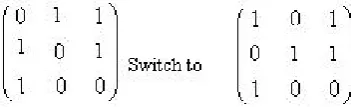
The switching component of binary matrix with two non parallel directions is the set of four points. The

four points makes a parallelogram whose two opposite sides are parallel to one direction and other two sides are parallel to other direction. The value of points of two edges of the line of the parallelogram is opposite.

1.a Switching component for horizontal and vertical directions

.b Switching componentfor diagonal

and anti diagonal directions c Switching component_{and horizontal directions}for diagonal

Figure 1 Switching component for two non parallel directions.

If 𝑆𝑆=�𝑓𝑓_𝑖𝑖_,_𝑖𝑖,𝑓𝑓_𝑖𝑖_1,_𝑖𝑖₁,𝑓𝑓_𝑖𝑖_2,_𝑖𝑖₂,𝑓𝑓_𝑖𝑖_3,_𝑖𝑖₃� is the switching component with two non parallel direction then changing the values of each elements of switching component

from one to zero or zero to one is called switching operation such as

𝑓𝑓𝑖𝑖,𝑖𝑖 = 1− 𝑓𝑓𝑖𝑖,𝑖𝑖 , 𝑓𝑓𝑖𝑖1,𝑖𝑖1= 1− 𝑓𝑓𝑖𝑖1,𝑖𝑖1 , 𝑓𝑓𝑖𝑖2,𝑖𝑖2= 1− 𝑓𝑓𝑖𝑖2,𝑖𝑖2 , 𝑓𝑓𝑖𝑖3,𝑖𝑖3= 1− 𝑓𝑓𝑖𝑖3,𝑖𝑖3 (6)

After switching operation the binary matrix remain tomographically equivalent with respect to these

two non parallel direction means their values of the projections with these two directions does not change

Figure 2 Switching operations with horizontal and vertical directions.

3.1 Switching Component with the horizontal and vertical directions

Let A point 𝑓𝑓_𝑖𝑖_,_𝑖𝑖 = 1�𝑓𝑓_𝑖𝑖_._𝑖𝑖 = 0� in the binary matrix 𝐹𝐹=�𝑓𝑓_{𝑖𝑖𝑖𝑖}�

(3)

195 Copyright © 2016. Vandana Publications. All Rights Reserved.

• 𝑓𝑓𝑘𝑘,𝑙𝑙 = 1(𝑓𝑓𝑘𝑘.𝑙𝑙 = 0)

• 𝑓𝑓𝑖𝑖,𝑙𝑙= 0(𝑓𝑓𝑖𝑖.𝑙𝑙 = 1)

• 𝑓𝑓𝑘𝑘,𝑖𝑖 = 0�𝑓𝑓𝑘𝑘.𝑖𝑖 = 1�

∀ 1≤ 𝑘𝑘 ≤ 𝑚𝑚,𝑘𝑘 ≠ 𝑖𝑖 , 1≤ 𝑙𝑙 ≤ 𝑛𝑛 ,𝑙𝑙 ≠ 𝑖𝑖, 1≤ 𝑖𝑖 ≤ 𝑚𝑚𝑎𝑎𝑛𝑛𝑑𝑑 1≤ 𝑖𝑖 ≤ 𝑛𝑛

Then set 𝑆𝑆=�𝑓𝑓_𝑖𝑖_,_𝑖𝑖,𝑓𝑓_𝑘𝑘_,_𝑙𝑙,𝑓𝑓_𝑖𝑖_,_𝑙𝑙,𝑓𝑓_𝑘𝑘_,_𝑖𝑖� is called switching component of matrix A with respect to directions (1,0) and (0,1) or horizontal and vertical. If we switch the elements of switching component with respect to directions (1,0) and (0,1) then the value of R (row sum) and C (column sum) remain the same.

3.2 Switching Component with the diagonal and anti diagonal directions

Let A point 𝑓𝑓_𝑖𝑖_,_𝑖𝑖 = 1�𝑓𝑓_𝑖𝑖_._𝑖𝑖 = 0� in the binary matrix 𝐹𝐹=�𝑓𝑓_{𝑖𝑖𝑖𝑖}�

𝑚𝑚×𝑛𝑛 . If there exist two number k>0 and l >0such that

• 𝑓𝑓𝑖𝑖1,𝑖𝑖1= 1�𝑓𝑓𝑖𝑖1.𝑖𝑖1= 0� | 𝑖𝑖1 =𝑘𝑘+𝑙𝑙+𝑖𝑖, 𝑖𝑖1 =𝑘𝑘 − 𝑙𝑙+𝑖𝑖 ∀ 1≤ 𝑖𝑖1≤ 𝑚𝑚, 1≤ 𝑖𝑖1≤ 𝑛𝑛

• 𝑓𝑓𝑖𝑖2,𝑖𝑖2= 0�𝑓𝑓𝑖𝑖2,𝑖𝑖2= 1� | 𝑖𝑖2 =𝑘𝑘+𝑖𝑖, 𝑖𝑖2 =𝑘𝑘+𝑖𝑖 ∀ 1≤ 𝑖𝑖2≤ 𝑚𝑚, 1≤ 𝑖𝑖2≤ 𝑛𝑛

• 𝑓𝑓𝑖𝑖3,𝑖𝑖3= 0(𝑓𝑓𝑖𝑖3,𝑖𝑖3= 1) | 𝑖𝑖3 =𝑙𝑙+𝑖𝑖, 𝑖𝑖3 =−𝑙𝑙+𝑖𝑖 ∀ 1≤ 𝑖𝑖3≤ 𝑚𝑚, 1≤ 𝑖𝑖3≤ 𝑛𝑛

∀ 1≤ 𝑖𝑖 ≤ 𝑚𝑚, 1≤ 𝑖𝑖 ≤ 𝑛𝑛

Then set 𝑆𝑆=�𝑓𝑓_𝑖𝑖_,_𝑖𝑖,𝑓𝑓_𝑖𝑖_1,_𝑖𝑖₁,𝑓𝑓_𝑖𝑖_2,_𝑖𝑖₂,𝑓𝑓_𝑖𝑖_3,_𝑖𝑖₃� is called switching component of matrix A with respect to directions (1,1) and (1,-1) or diagonal and anti diagonal. If we switch the elements of switching component with respect to directions (1,0) and (0,1) then the value of D (diagonal sum) and A (anti diagonal sum) remain the same.

3.3 Switching Component with any arbitrary two non

parallel directions

Let A point 𝑓𝑓_𝑖𝑖_,_𝑖𝑖 = 1�𝑓𝑓_𝑖𝑖_._𝑖𝑖 = 0�in the binary matrix 𝐹𝐹=�𝑓𝑓_{𝑖𝑖𝑖𝑖}�

𝑚𝑚×𝑛𝑛 and two non parallel direction

𝑣𝑣1= {𝑣𝑣11,𝑣𝑣12} and 𝑣𝑣2= {𝑣𝑣21,𝑣𝑣22} If there exist two

number k>0 and l >0 such that

• 𝑓𝑓𝑖𝑖1,𝑖𝑖1= 1 �𝑓𝑓𝑖𝑖1.𝑖𝑖1= 0� | 𝑖𝑖1 =𝑘𝑘𝑣𝑣11+𝑙𝑙𝑣𝑣12+𝑖𝑖, 𝑖𝑖1 =𝑘𝑘𝑣𝑣21+𝑙𝑙𝑣𝑣22+𝑖𝑖 ∀ 1≤ 𝑖𝑖1≤ 𝑚𝑚, 1≤ 𝑖𝑖1≤ 𝑛𝑛

• 𝑓𝑓𝑖𝑖2,𝑖𝑖2= 0 �𝑓𝑓𝑖𝑖2,𝑖𝑖2= 1� | 𝑖𝑖2 =𝑘𝑘𝑣𝑣11+𝑖𝑖, 𝑖𝑖2 =𝑘𝑘𝑣𝑣21+𝑖𝑖 ∀ 1≤ 𝑖𝑖2≤ 𝑚𝑚, 1≤ 𝑖𝑖2≤ 𝑛𝑛

• 𝑓𝑓𝑖𝑖3,𝑖𝑖3= 0 (𝑓𝑓𝑖𝑖3,𝑖𝑖3= 1) | 𝑖𝑖3 =𝑙𝑙𝑣𝑣12+𝑖𝑖, 𝑖𝑖3 =𝑙𝑙𝑣𝑣22+𝑖𝑖 ∀ 1≤ 𝑖𝑖3≤ 𝑚𝑚, 1≤ 𝑖𝑖3≤ 𝑛𝑛

∀ 1≤ 𝑖𝑖 ≤ 𝑚𝑚, 1≤ 𝑖𝑖 ≤ 𝑛𝑛

Then set 𝑆𝑆=�𝑓𝑓_𝑖𝑖_,_𝑖𝑖,𝑓𝑓_𝑖𝑖_1,_𝑖𝑖₁,𝑓𝑓_𝑖𝑖_2,_𝑖𝑖₂,𝑓𝑓_𝑖𝑖_3,_𝑖𝑖₃� is called switching component of matrix A with respect to two non parallel direction 𝑣𝑣₁= {𝑣𝑣₁₁,𝑣𝑣₁₂} and𝑣𝑣₂=

{𝑣𝑣21,𝑣𝑣22}. If we switch the elements of switching

component with respect to two non parallel directions

𝑣𝑣1= {𝑣𝑣11,𝑣𝑣12} and 𝑣𝑣2= {𝑣𝑣21,𝑣𝑣22} then the value of

projections with respect to direction v1 and v2 remain the same.

IV. BINARY PSO BASED IMAGE

RECONSTRUCTION

In this paper PSO based Image reconstruction algorithm is proposed, which is the population based

relatively recent category of stochastic global optimisation algorithm. Particle Swarm Optimisation is inspired by social and cooperative behaviour of some species which are moving in group to search their foods. Some of these are swarm of birds, school of fish, cooperative behaviour of ants and bees etc. The particles or members of the swarm fly through a multidimensional search space to find some optimal solution. Each particle changes its position in the search space from time to time according to the flying experience of its own and its neighbours.

The next position of the particles in the search space is calculated with the help of particle velocity and displacement equations

𝑉𝑉𝑝𝑝(𝑖𝑖+ 1) =𝑤𝑤 ∙ 𝑉𝑉𝑝𝑝(𝑖𝑖) +𝑐𝑐1∙ 𝑟𝑟1(𝑥𝑥𝑙𝑙𝑝𝑝(𝑖𝑖)− 𝑥𝑥𝑝𝑝(𝑖𝑖)) +𝑐𝑐2∙ 𝑟𝑟2(𝑥𝑥𝑔𝑔𝑝𝑝(𝑖𝑖)− 𝑥𝑥𝑝𝑝(𝑖𝑖)) (7)

𝑥𝑥𝑝𝑝(𝑖𝑖+ 1) = 𝑥𝑥𝑝𝑝(𝑖𝑖) +𝑉𝑉𝑝𝑝(𝑖𝑖+ 1) (8)

These positions have been obtained on the basis of an additive influence of three components: (i) Present velocity, (ii) Distance between its present position and its personal best position xlp(i)). (iii) Distance between its present position and global best position of the particle xg(i) among the entire swarm found so far.

According to flying experience best local solution (local maxima or minima) and best global solution (global maxima or minima) of each particle is

stored in the memory. The particles are interacted to each other with this local or global maxima or minima. Each particle evaluates other particle with some fitness function, which is quality measure of the solution and compare with its own fitness values [16,17].

(4)

196 Copyright © 2016. Vandana Publications. All Rights Reserved.

in this case is calculated some difference way as calculated in continues PSO [18, 19].

𝛥𝛥𝑉𝑉𝑝𝑝(𝑖𝑖+ 1) =𝑐𝑐1∙ 𝑟𝑟1(𝑥𝑥𝑙𝑙𝑝𝑝(𝑖𝑖)− 𝑥𝑥𝑝𝑝(𝑖𝑖)) +𝑐𝑐2∙ 𝑟𝑟2(𝑥𝑥𝑔𝑔𝑝𝑝(𝑖𝑖)− 𝑥𝑥𝑝𝑝(𝑖𝑖)) (9)

𝑉𝑉𝑝𝑝(𝑖𝑖+ 1) = h(𝑉𝑉𝑝𝑝(𝑖𝑖) +𝛥𝛥𝑉𝑉𝑝𝑝(𝑖𝑖+ 1)) (10) 𝑥𝑥_𝑝𝑝(𝑖𝑖+ 1) =�1 𝑖𝑖𝑓𝑓 𝑟𝑟𝑎𝑎𝑛𝑛𝑑𝑑𝑟𝑟𝑚𝑚(1) <𝑠𝑠𝑖𝑖𝑔𝑔𝑚𝑚𝑟𝑟𝑖𝑖𝑑𝑑(𝑉𝑉𝑝𝑝(𝑖𝑖+ 1))

0 𝑟𝑟𝑜𝑜ℎ𝑒𝑒𝑤𝑤𝑖𝑖𝑠𝑠𝑒𝑒 � (11)

Here sigmoid (𝑉𝑉_𝑝𝑝(𝑖𝑖+ 1)) = 1

1+𝑒𝑒−𝑉𝑉𝑝𝑝(𝑖𝑖+1) and random (1) is random number between 0 and 1.

𝛥𝛥𝑉𝑉𝑝𝑝(𝑖𝑖+ 1) is the change in the velocity of the particles

Figure 3. Particle move toward their personal best (Pbest) and global best (gbest)

4.1 Evaluation Criteria new Binary Particle Swarm optimization

The following projection errors to measure the quality of solution are defined

𝑒𝑒

𝑟𝑟

=

∑

𝑚𝑚𝑖𝑖=1

|

𝑟𝑟

′

𝑖𝑖

− 𝑟𝑟

𝑖𝑖

|

,

𝑒𝑒

𝑐𝑐

=

∑ �𝑐𝑐

𝑛𝑛𝑖𝑖=1 ′𝑖𝑖

− 𝑐𝑐

𝑖𝑖

�

,

𝑒𝑒

𝑑𝑑

=

∑

|

𝑑𝑑

′

𝑘𝑘

− 𝑑𝑑

𝑘𝑘

|

,

𝑒𝑒

𝑎𝑎

=

∑

|

𝑎𝑎

′

𝑘𝑘

− 𝑎𝑎

𝑘𝑘

|

and the fitness function is taken as

𝐹𝐹𝑖𝑖𝑜𝑜𝑛𝑛𝑒𝑒𝑠𝑠𝑠𝑠

=

𝑒𝑒

𝑟𝑟

+

𝑒𝑒

𝑐𝑐

+

𝑒𝑒

𝑑𝑑

+

𝑒𝑒

𝑎𝑎 (12)

Where ri , cj , dk and ak , denote the ith row sum , jth column sum, kth diagonal sum , and kth anti diagonal sum respectively, and ri’ , cj’ , dk’ and ak’ denote the same from reconstructed binary matrix. er ,ec , ed and ea are projections error in row sums, column sums, diagonal sums and anti diagonal sums respectively. If the value of fitness function is low then fitness of binary matrix will be high.

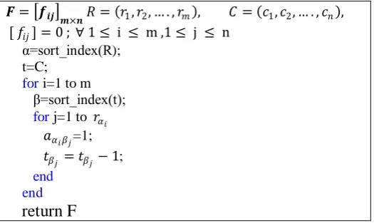
4.2 Initial Population

The starting solution of reconstruction initiated with some solutions of image reconstruction from orthogonal projections such that either row and column

sums or diagonal and anti diagonal sums. We used row sum and column sum to find out initial solutions. To find this solution first we create a binary matrix 𝑭𝑭=�𝒇𝒇_{𝒊𝒊𝒊𝒊}�

𝒎𝒎×𝒏𝒏 with all elements equal to zero. Reconstruction algorithm is given in the figure 2. it use array R and C as input and return reconstructed binary matrix as output. In this algorithm sort_index is a function which sort the array in descending order according to their values but return their index values of original array not data values. Example if z={13,15,16,12,14,11} then it will return zi={3,2,5,1,4,6}.

𝑭𝑭=�𝒇𝒇𝒊𝒊𝒊𝒊�_𝒎𝒎_×_𝒏𝒏𝑅𝑅= (𝑟𝑟1,𝑟𝑟2, … . ,𝑟𝑟𝑚𝑚), 𝐶𝐶= (𝑐𝑐1,𝑐𝑐2, … . ,𝑐𝑐𝑛𝑛),

[ 𝑓𝑓𝑖𝑖𝑖𝑖] = 0 ; ∀ 1≤ i ≤ m ,1≤ j ≤ n

α=sort_index(R); t=C;

for i=1 to m β=sort_index(t);

for j=1 to 𝑟𝑟_𝛼𝛼_𝑖𝑖 𝑎𝑎_𝛼𝛼_𝑖𝑖_𝛽𝛽_𝑖𝑖=1; 𝑜𝑜_𝛽𝛽_𝑖𝑖 =𝑜𝑜_𝛽𝛽_𝑖𝑖 −1; end

end

return F

(5)

197 Copyright © 2016. Vandana Publications. All Rights Reserved.

After reconstruction of this binary matrix from their row and column sum switching operations with horizontal and vertical directions is performed with number of times to get different solutions with same row and column sum and these different solution make out

initial population of out particle swarm optimization algorithm. All these solutions are tomographically equivalent with respect to row projection and column projection

X0_{= {}_𝑥𝑥

10,𝑥𝑥20,𝑥𝑥30… …𝑥𝑥𝑛𝑛𝑟𝑟0 } ∀𝑥𝑥ℎ0= randomswitch(F,k) (13) Here randomswitch (F,k) is a function which perform k time random switching on F

P0_{= X}0₍₁₄₎

𝑓𝑓𝑖𝑖𝑜𝑜𝑛𝑛𝑒𝑒𝑠𝑠𝑠𝑠(𝑝𝑝𝑔𝑔0) = min⁡{𝑓𝑓𝑖𝑖𝑜𝑜𝑛𝑛𝑒𝑒𝑠𝑠𝑠𝑠(𝑝𝑝10),𝑓𝑓𝑖𝑖𝑜𝑜𝑛𝑛𝑒𝑒𝑠𝑠𝑠𝑠(𝑝𝑝20), … … … …𝑓𝑓𝑖𝑖𝑜𝑜𝑛𝑛𝑒𝑒𝑠𝑠𝑠𝑠(𝑝𝑝𝑛𝑛𝑟𝑟0 )} (15)

Here X0 is set of initial solution, P0 is the set of personal best solutions by the particles and 𝑝𝑝_𝑔𝑔0 is global best solution among all solutions for initial populations

4.3 Finding new solutions

The new solution in binary particle swarm optimization algorithm is find out with new velocity and position of each multi dimensional particles

𝑣𝑣ℎ𝑖𝑖𝑖𝑖𝑘𝑘 =�1 𝑖𝑖𝑓𝑓 𝑏𝑏 �

R1hijC1�phij 𝒙𝒙𝒙𝒙𝒙𝒙𝑥𝑥ℎ𝑖𝑖𝑖𝑖�+ R2hijC2�pgij 𝒙𝒙𝒙𝒙𝒙𝒙𝑥𝑥ℎ𝑖𝑖𝑖𝑖�

C1+C2 �> R3hij

0 𝑟𝑟𝑜𝑜ℎ𝑒𝑒𝑤𝑤𝑖𝑖𝑠𝑠𝑒𝑒 � (16) 𝑥𝑥ℎ𝑖𝑖𝑖𝑖𝑘𝑘 =𝑥𝑥ℎ𝑖𝑖𝑖𝑖𝑘𝑘 𝑥𝑥𝑟𝑟𝑟𝑟𝑣𝑣ℎ𝑖𝑖𝑖𝑖𝑘𝑘 (17)

∀ 1≤ 𝑖𝑖 ≤ 𝑚𝑚, 1≤ 𝑖𝑖 ≤ 𝑛𝑛

Here C₁and C₂ are the social and cognitive parameters, b is momentum parameter, and

R1, R2 and R3 are uniform random numbers between

(0,1).

Personal best and global best particles are updated as shown in next equations.

𝑝𝑝ℎ𝑘𝑘 =�𝑥𝑥ℎ

𝑘𝑘 _{𝑖𝑖𝑓𝑓}_{𝑓𝑓𝑖𝑖𝑜𝑜𝑛𝑛𝑒𝑒𝑠𝑠𝑠𝑠}₍_𝑝𝑝

ℎ𝑘𝑘) >𝑓𝑓𝑖𝑖𝑜𝑜𝑛𝑛𝑒𝑒𝑠𝑠𝑠𝑠(𝑥𝑥ℎ𝑘𝑘)

𝑝𝑝ℎ𝑘𝑘 𝑟𝑟𝑜𝑜ℎ𝑒𝑒𝑤𝑤𝑖𝑖𝑠𝑠𝑒𝑒 �

∀ 1≤ ℎ ≤ 𝑛𝑛𝑟𝑟, (18)

𝑔𝑔= �ℎ 𝑖𝑖𝑓𝑓 𝑓𝑓𝑖𝑖𝑜𝑜𝑛𝑛𝑒𝑒𝑠𝑠𝑠𝑠(𝑝𝑝𝑔𝑔𝑘𝑘) >𝑓𝑓𝑖𝑖𝑜𝑜𝑛𝑛𝑒𝑒𝑠𝑠𝑠𝑠(𝑝𝑝ℎ𝑘𝑘)

𝑔𝑔 𝑟𝑟𝑜𝑜ℎ𝑒𝑒𝑤𝑤𝑖𝑖𝑠𝑠𝑒𝑒 � ∀ 1≤ ℎ,𝑔𝑔 ≤ 𝑛𝑛𝑟𝑟, (19)

Here g is the index value of global best particle in the personal best particles, hence 𝑝𝑝_𝑔𝑔𝑘𝑘 will be the global best particle among all the particles.

4.4 Random Switching on the particles

After some iteration the particle reached in the position of local minima to avoid such situation we need some random move in the particles, for this we use switching operations in particles as given in (2.3). we can also perform mutation operation on the particle but

switching operation does not alter the projections values in the directions at which operation is performed. The random two directions are selected from the set of four directions. Then random switching component is found out with these two random directions. After that random switching is performed on the particles for which

𝑓𝑓𝑖𝑖𝑜𝑜𝑛𝑛𝑒𝑒𝑠𝑠𝑠𝑠�𝑝𝑝𝑔𝑔𝑘𝑘�=𝑓𝑓𝑖𝑖𝑜𝑜𝑛𝑛𝑒𝑒𝑠𝑠𝑠𝑠(𝑝𝑝𝑛𝑛𝑘𝑘) to move the particle in random directions

𝑥𝑥_ℎ𝑘𝑘=�𝑟𝑟𝑎𝑎𝑛𝑛𝑑𝑑𝑟𝑟𝑚𝑚𝑠𝑠𝑤𝑤𝑖𝑖𝑜𝑜𝑐𝑐ℎ(𝑥𝑥ℎ

𝑘𝑘₎ _{𝑖𝑖𝑓𝑓}_{𝑓𝑓𝑖𝑖𝑜𝑜𝑛𝑛𝑒𝑒𝑠𝑠𝑠𝑠�𝑝𝑝}

𝑔𝑔𝑘𝑘�=𝑓𝑓𝑖𝑖𝑜𝑜𝑛𝑛𝑒𝑒𝑠𝑠𝑠𝑠(𝑥𝑥ℎ𝑘𝑘)

𝑥𝑥ℎ𝑘𝑘 𝑟𝑟𝑜𝑜ℎ𝑒𝑒𝑤𝑤𝑖𝑖𝑠𝑠𝑒𝑒 �

∀ 1≤ ℎ ≤ 𝑛𝑛𝑟𝑟, (20)

While (termination condition is false)

for h=1 to no for i=1 to m

for j=1 to n

if𝑏𝑏 ∗ �R1hijC1�Phij 𝒙𝒙𝒙𝒙𝒙𝒙𝑥𝑥ℎ𝑖𝑖𝑖𝑖�+ R2hijC2�Pgij 𝒙𝒙𝒙𝒙𝒙𝒙𝑥𝑥ℎ𝑖𝑖𝑖𝑖�

C1+C2 �> R3hij vhij=1;

else

vhij=0;

end

𝑥𝑥_{ℎ𝑖𝑖𝑖𝑖} =𝑥𝑥_{ℎ𝑖𝑖𝑖𝑖}𝑥𝑥𝑟𝑟𝑟𝑟𝑣𝑣_{ℎ𝑖𝑖𝑖𝑖}

(6)

if opt(xh) < opt(Ph) Ph = xh;

if opt(xh) < opt(Pg) g = h;

end

elseif opt(xh) = opt(Pg) xh=switchrandom(xh); end

end end

Figure 5 Binary PSO algorithm for image reconstruction

V. EXPERIMENTAL STUDY AND

RESULT

For experimental study, the test set of binary matrix of size 20X20, 30X30,40X40,50X50 and 60X60are generated and their projections calculated.

This Binary PSO based algorithm is tested with different number of iterations on these test sets.

Reconstruction: The reconstruction of the binary images from four projections using Binary PSO based algorithm are shown below

Size of images

Original Image Reconstructed image

20X20

30X30

40X40

60X60

Figure 6: Test images and their reconstructions with new algorithm

The values of personal best and global best are tested with different values of momentum parameter. This show that if value of parameter is very low then it

converges after large number of iterations on the other hand if parameter value is increases then number of iteration for convergence is decreases

Number of iterations

Value of Momentum parameter

(b=0.1)

(b=0.2)

Value of Momentum parameter (b=0.3)

Value of Momentum parameter (b=1)

0 58.1 58.1 58.1 58.1

500 22.1 20.1 21.1 23..4

1000 20.7 16.5 16 14

1500 17.9 14.8 16 14

2000 16 13.9 16 14

(7)

3000 14 10 16 14

3500 14 10 14 12

4000 14 10 14 12

4500 14 10 10 12

5000 14 10 10 12

Table 1 Average value of personal best fitness values with different values of momentum parameter

(b=0.1)

(b=0.2)

0 26 26 26 26

500 20 18 20 22

1000 20 16 16 14

1500 16 14 16 14

2000 16 12 16 14

2500 14 10 16 14

3000 14 10 16 14

3500 14 10 14 12

4000 14 10 14 12

4500 14 10 10 12

5000 14 10 10 12

Table 2 Global best fitness values with different values of momentum parameter

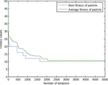
The convergence of fitness function is shown in following graphs. The graph shows the convergence of the fitness function in this new algorithm using BPSO. As the number of iteration increase the average fitness

value decreases, after a sufficient number of iterations the fitness value stabilized, this is point of the termination for BPSO based algorithm

Figure 7: Fitness values and Number of Iteration for 20X20 Binary test Image

0 500 1000 1500 2000 2500 3000 3500 4000 4500 5000

0 5 10 15 20 25 30 35 40 45 50

F

it

nes

s

v

al

ues

(8)

0 500 1000 1500 2000 2500 3000 3500 4000 4500 5000

10 20 30 40 50 60 70

Number of Itarations

F

it

nes

s

v

al

ues

best fitness of particle average fitness of particle

0 500 1000 1500 2000 2500 3000 3500 4000 4500 5000

20 40 60 80 100 120 140 160

F

it

nes

s

v

al

ues

(9)

VI. CONCLUSIONS

This is new approach in discrete tomography, to solve the problem using binary particle swarm optimization. This technique is easy to implement as compare to other evolutionary technique. Switching used in this approach is same as mutation used in genetic algorithm to diversify the solutions. It avoids the solutions to fall in local minima.

REFERENCES

[1] A.C. Kak and M. Slaney, Principles of Computerized Tomographic Imaging, IEEE Press, New York 1988. [2] A. Kuba and G.T.Herma, Discrete Tomography: Foundations, Algorithms and Applications, Birkhauser,Bosten, 1999.

[3] J. Hadamard, Lectures on Cauchy's problem in linear partial differential equations. Yale University Press, New Haven 1923.

[4] H.J. Ryser, Combinatorial properties of matrices of zero and ones, Canadian Journal of Mathematics 9 (1957) 371-377.

[5] D. Gale, A theorem on flows in networks, Pacific Journal of Mathematics 7 (1957) 1073-1082.

[6] S.K. Chang, The reconstruction of binary patterns from their projections, Communications of the ACM 14 (1971) 21–25.

[7] F. Jarray and G. Tlig, A simulated annealing for reconstructing hv-convex binary matrix , Electronic notes in Discrete Mathematics 33 (2010) 447-454. [8] E. Barcucci, A. Del Lungo, M. Nivat and R. Pinzani, Reconstructing convex polyominoes from their horizontal and vertical projections, Theoretical Computer Science 155 (1996) 321-347.

[9] S. Brunetti and A. Daurat, An algorithm reconstructing convex lattice sets, Theoretical Computer Science 304 (2003) 35-57.

[10] M. Chrobak and C. Dürr, Reconstructing hv-convex polyominoes from orthogonal projections, Information Processing Letter 69 (1999) 283-289.

[11] A. Del Lungo, A. Frosini, M. Nivat and L. Vuillon, Discrete Tomography: Reconstruction under Periodicity Constraints, Lecture Notes in Computer Science (2002) 38-56.

[12] N. Kumar and T. Srivastava, Image reconstruction from noisy projections under periodicity constraints using genetic algorithm, International journal of imaging and robotics 5(2011) 18-27.

[13] M. Venere, H, Liao and A, Clausse, A Genetic algorithm for adaptive tomography of elliptical objects,

IEEE Signal Processing Lette., Volume 7 (2000) 176–

178.

[14] C. Valenti, A genetic algorithm for discrete tomography reconstruction, Genetic Programming and EvolvableMachines. Volume 9 (2008) 85-96.

0 500 1000 1500 2000 2500 3000 3500 4000 4500 5000

50 100 150 200 250 300 350

number of iterations

fi

tnes

s

v

al

ues

(10)

[15] K. J. Batenburg, An evolutionary algorithm for discrete tomography, Discrete Applied Mathematics archive, Volume 151(2005) 36–54.

[16] J. Kennedy and R.C. Eberhart, Particle swarm optimization. In: IEEE International Conference on Neural Network, Perth, Australia (1995) 1942–1948. [17] M. Clerc and J. Kennedy, The particle swarm-explosion, stability and convergence in a multidimensional complex space. IEEE Transactions on Evolutionary Computation 6 (2002) 58–73.

[18] M.F.Tasgetiren, Y-Ch. Liang, A binary particle swarm optimization algorithm for lot sizing problem, Journal of Economic and Social Research 5 (2) (2003) 1–20.