Bounding Uncertainty for Active Batch Selection

(1)

The Thirty-Third AAAI Conference on Artificial Intelligence (AAAI-19)

Bounding Uncertainty for Active Batch Selection

Hanmo Wang,

1,2

Runwu Zhou,

1,2

Yi-Dong Shen

1∗

1_{State Key Laboratory of Computer Science, Institute of Software, Chinese Academy of Sciences, China} 2_{University of Chinese Academy of Sciences, Beijing 100049, China}

{wanghm,zhourw,ydshen}@ios.ac.cn

Abstract

The success of batch mode active learning (BMAL) methods lies in selecting both representative and uncertain samples. Representative samples quickly capture the global structure of the whole dataset, while the uncertain ones refine the deci-sion boundary. There are two principles, namelythe direct approachand the screening approach, to make a trade-off between representativeness and uncertainty. Although widely used in literature, little is known about the relationship be-tween these two principles. In this paper, we discover that the two approaches both have shortcomings in the initial stage of BMAL. To alleviate the shortcomings, we bound the cer-tainty scores of unlabeled samples from below and directly combine this lower-bounded certainty with representative-ness in the objective function. Additionally, we show that the two aforementioned approaches are mathematically equiva-lent to two special cases of our approach. To the best of our knowledge, this is the first work that tries to generalize the di-rect and screening approaches. The objective function is then solved by super-modularity optimization. Extensive experi-ments on fifteen datasets indicate that our method has signif-icantly higher classification accuracy on testing data than the latest state-of-the-art BMAL methods, and also scales better even when the size of the unlabeled pool reaches106.

Introduction

Active learning (Settles 2010) is a machine learning and data mining methodology to automatically select informative data instances for annotation when facing a large amount of unlabeled data. The goal of active learning is to train a classi-fier that has good generalization performance with informa-tive instances only. Traditional acinforma-tive learning methods it-eratively select one single informative instance and thus are not efficient when there are multiple annotators. Recently, batch mode active learning (BMAL) was introduced, which makes the annotation process more productive by selecting multiple instances in each iteration.

Informative instances in BMAL are both representative and uncertain. The representativeness indicates that the se-lected instances capture some global structure of the

en-∗

Corresponding author

tire dataset, while the uncertainty indicates that the se-lected instances can refine the decision boundary in a label-efficient way. Empirically, choosing representative instances are particularly critical when labeled data is scarce, while uncertainty plays a more important role as the number of labeled instances increases (Guo and Schuurmans 2008; Wang and Ye 2015; Settles 2010). There are two common approaches to combine representativeness and (un)certainty. The first is the direct approach, which directly combines representativeness with uncertainty to form a single objec-tive, such as in (Wang and Ye 2015), (Chakraborty et al. 2015a) and (Chakraborty et al. 2015b). The second is the

screening approach, which excludes some unlabeled

in-stances about which the classifier is certain, and chooses representative samples among the remaining instances, such as in (Chattopadhyay et al. 2012) and (Chakraborty et al. 2015b). Neither of these two approaches can handle small number of labeled instances in the beginning of BMAL, when the labeled data is scarce. Under such circumstances, there are not adequate labeled data to train an accurate clas-sifier, and thus the output of the classifier is usually not accu-rate. The direct approach, which directly utilizes the output, is therefore possibly misled; the screening approach, which screens samples beforehand, may accidentally remove use-ful instances.

(2)

BMAL method treats the noisy samples with equal certainty and thus eliminates some of the most misleading certainty scores. On the other hand, our method takes all unlabeled samples into account, so it may not accidentally discard use-ful instances merely by their certainty scores as the screen-ing approach does.

As well as the quality of the selected samples, the ef-ficiency of BMAL methods also matters in practice. Un-fortunately, most of the existing BMAL methods are not scalable. For example, the most recent methodbatchRank

in (Chakraborty et al. 2015b) runs in O(n2

u), where nu

is the number of unlabeled instances. The MMD-based BMAL method (Chattopadhyay et al. 2012) and its vari-ant (Wang and Ye 2015) both use a Quadratic Program-ming toolbox which runs inO(n3

u). Another representative

BMAL method (Wang et al. 2015) tends to solve its ob-jective function using the sub-gradient method, which has a slow convergence rate. To illustrate the effectiveness, we instantiate our method by choosing Maximum Mean Dis-crepancy (MMD) (Gretton et al. 2006)(Gretton et al. 2012) as representativeness and posterior probabilities to the most likely class as certainty. Under mild conditions, we prove the super-modularity of our objective function and utilize a random greedy method (Buchbinder et al. 2014) to obtain a fast solution. Our method scales linearly w.r.t.nu and can handle more than106_{unlabeled instances.}

Our contributions are as follows:

• We propose to bound the uncertainty of the unlabeled samples for active learning. Such mechanism not only al-leviates the problem with the noisy output of the classifier, but also takes all unlabeled samples into consideration. In other words, our method alleviates the problems with the direct approach and the screening approach.

• Our framework can be seen as a generalization of the two aforementioned approaches. To the best of our knowl-edge, this is the first work for such generalizations. For effectiveness, we empirically choose MMD (Chattopad-hyay et al. 2012) and the least confident method as rep-resentativeness and uncertainty, respectively. In addition, we discover a trivial solution of the original Quadratic Programming solver in (Chattopadhyay et al. 2012) and propose to solve the objective with a random greedy solver that has theoretical guarantees.

• We conduct extensive experiments on fifteen bench-mark datasets. The result demonstrates that our method with LBC has significantly higher accuracy than the lat-est state-of-the-art BMAL methods, while managing to achieve faster (sometimes in several order of magnitude) running time.

Related Work

Active learning has been an important topic in machine learning and data mining. One extensively studied category is pool-based active learning (Settles 2010), where an active learner is exposed to a large pool of unlabeled data, and it

automatically decides which instances are the most informa-tive for labeling. Pool-based acinforma-tive learning methods can be roughly categorized into two groups. One issingle instance

selection, where a single informative instance is selected

it-eratively to update the classifier. Well-known single instance selection methods include query-by-committee (Seung, Op-per, and Sompolinsky 1992) and uncertainty sampling (Tong and Koller 2002). The other category is multiple instance

selection, a.k.a. batch mode active learning (BMAL), where

multiple annotators are available and the learner iteratively selects multiple instances instead of one.

There is a variety of pioneer work in BMAL, which also considers representativeness and uncertainty. For ex-ample, (Guo and Schuurmans 2008) proposes to select in-stances based on pure discriminativeness (which can be seen as a variant of uncertainty). Later, (Guo 2010) pro-poses an approach to selecting a batch of samples that min-imizes the mutual information between labeled and unla-beled data. (Hoi et al. 2006) apply the Fisher information as an uncertainty criterion in BMAL. Recently, (Chattopad-hyay et al. 2012) propose a representative method to mini-mize the difference in distribution between labeled and un-labeled data via selecting the samples with the lowest MMD score. (Wang and Ye 2015) further combine this distribution-matching method with discriminative information. Another method based on the distribution-matching criterion named relative Pearson divergence is proposed in (Wang et al. 2015). (Chakraborty et al. 2015b) present a method using mutual information and entropy. There are also other BMAL methods for specified classifiers such as hierarchical classifi-cation (Cheng et al. 2014)(Chakraborty et al. 2015a), logistic regression (Gu, Zhang, and Han 2014), multi-class classifier (Reyes and Ventura 2018; Yan and Huang 2018) and Naive Bayes/Nearest Neighbor (Wei, Iyer, and Bilmes 2015). Re-cently, there is also theoretical analysis of BMAL(Chen and Krause 2013).

Batch Mode Active Learning

Before diving into our method, we introduce the formal problem setting for BMAL. Let X = {x1,x2, ...,xn} be

a dataset of n instances with dimensionalityd. We useL

andU to denote sets of labeled and unlabeled indexes re-spectively, whereL∪U = {1,2, ..., n}andL∩U = ∅. Letnl =|L|andnu =|U|. LetXLandXU be the labeled and unlabeled set respectively, i.e.,XL ={xi|i ∈ L}and

XU ={xi|i∈U}. Each instancexiis associated with label

yi ∈ {1, ...,|y|}. Ifxi ∈XL, labelyi is revealed by a

hu-man labeler; otherwiseyiis unknown. A BMAL algorithm iteratively select a batch of samplesXS with indexesS

sat-isfyingS ⊂ U and|S| = buntil there is no budget (user specified) available for labeling, where the batch sizebis a predefined constant.

The Proposed Algorithm

For a candidate batchS ⊂ U, we defineR(S)andC(S)

(3)

We ignore the certainty score of some low-certainty samples by ensuring a lower bound on the certainty score of all un-labeled instances. Formally, for each instancexi ∈ XU we

propose the lower-bounded certainty (LBC) score as follows

LC(xi) = max(C(xi), ) (1)

with thresholdindicating the smallest accurate certainty. We mainly consider the most widely-used type of certainty, i.e., additive certainty, with the following definition.

Definition 1. Additive Certainty:We say certainty function

C(·) : 2U _{7→ R}_{to be additive iff}_{C(S) =}P

i∈SC(xi)for

anyS⊂U.

Additivity indicates that the certainty measure is calcu-lated in the instance level, and it applies to most of the certainty measures, such as entropy (Chakraborty et al. 2015b) and margin sampling (Scheffer, Decomain, and Wro-bel 2001).

With this nice property, we define the LBC on a setS⊂U

as

LC(S) =X

i∈S

max(C(xi), )

Without loss of generality, we directly combine the repre-sentativenessR(S)with LBC scoreLC(S)and obtain the BMAL framework with LBC:

min

S⊂U,|S|=bR(S) +λLC(S) (2)

whereλis a trade-off parameter.

Before instantiating our method with specific representa-tiveness and certainty, we prove that the direct and screening approaches are two special cases of our method in Eq. (2).

Lemma 1. For representativenessR(S)and additive

cer-taintyC(S), the direct approach with the following

objec-tive

min

S⊂U,|S|=bR(S) +λC(S), (3)

and the screening approach that optimizes

min

S⊂U,|S|=bR(S)

s.t. C(xi)≤for alli∈S

(4)

are both special cases of our method in Eq.(2).

Proof. the direct approach: the direct approach directly

combines representativeness with uncertainty. By setting threshold tomini∈UC(xi), we have C(xi) ≥ for all

i∈U, i.e.max(C(xi), ) =C(xi). The LBCLC(·) degen-erates to certaintyC(·), and thus Eq. (2) becomes equivalent to Eq. (3).

the screening approach:The screening approach mini-mizes merely representativeness over uncertain samples. Let

S∗ be the global optimizer of the screening approach in Eq. (4), and letv∗be the smallest violation in certainty, i.e.,

v∗ = minC(xi)>C(xi)−fori∈ U. When the trade-off

parameterλsatisfiesλ > R(S∗)/v∗, any instancexj with

c(xj)> will be heavily penalized such that for anyS

sat-isfyingj∈S, we havef(S) =R(S) +λLC(S)≥R(S) +

λLC(xj)≥R(S)+(R(S∗)/v∗)C(xj)> R(S)+R(S∗)≥

R(S∗) = R(S∗) +λLC(S∗) = f(S∗), i.e. any batch of

samples that contains the instance whose certainty is above

is not the global optimal of Eq. (2). Therefore, the solution to Eq. (2) is restricted to the instances with certainty lower than or equal to, i.e. optimizing the objective in Eq. (2) is equivalent to optimizing Eq. (4) whenλbecomes large.

The above lemma holds for most of the recent BMAL algorithms that utilize both representativeness and (un)certainty. (Wang and Ye 2015; Chakraborty et al. 2015a; 2015b; Chattopadhyay et al. 2012; Yang et al. 2015).

In the following, we instantiate our algorithm using spe-cific certainty and representativeness. For a probabilistic classifier with parameter w, we assume the true labels of unlabeled samples are drawn from categorical distributions, i.e

yi∼Categorical(pi) (5)

wherepiis the vector of the probability estimate ofxi

pi= [P(y= 0|xi,w);...;P(y=|y||xi,w)] (6)

In this paper, we use accuracy as the evaluation metric. Therefore, the expected accuracy on the unlabeled setU be-comes

ACC

V

U =Eyi∼Cat(pi),i∈U

1

|U|I(yi= ˆyi) (7)

whereyiˆ = arg max_yP(y|xi,w)is the predicted label. We can easily calculate the expected accuracy as

ACC

V

U =

1

|U|maxy P(y|xi,w) (8)

Following (Wang et al. 2018), the uncertainty ofxi is

de-fined as the expected accuracy onU\i. After droping con-stants, the uncertainty of samplexibecomes

C(xi) =ACC

V

U\i∼max_y P(y|xi,w) (9)

In the initial stage of BMAL, the certainty measure is usu-ally noisy because there is no adequate labeled data to train the classifier. Nevertheless, samples with high certainty usu-ally remain certain under a noisy classifier (trained with in-adequate data). To be more specific, the instances with high certainty are generally far away from the decision bound-ary, so they are highly likely to remain certain whether un-der a noisy classifier or the ground-truth classifier (trained with all data). As a result, even a noisy classifier predicts accurately the highly certain samples. On the other hand, uncertain samples are usually close to the decision bound-ary, which makes their certainty scores untrustworthy under a noisy classifier with an inaccurate decision boundary. To alleviate this issue, we bound the certainty scores from be-low

LC(S) =X

i∈S

(4)

In the beginning of the sample selection process, so-called representativeness are critical because it captures the global structure of the unlabeled data. We use a typical representa-tiveness measure named empirical MMD score ( See (Gret-ton et al. 2006)(Gret(Gret-ton et al. 2012) for more details), which selects instances that minimizes the difference in distribu-tion between labeled and unlabeled data:

R(S) :=MMD[φ, XL∪S, XU\S] =

1 2

X

i∈S

X

j∈S

Kij+

X

i∈S

hi

hi=

nu−b

n

X

j∈L

Kij−

nl+b

n

X

j∈U

Kij

(11) whereφ(·)is a kernel mapping andKis the kernel matrix that measures similarity over all instances.

After substituting Eq. (11) and Eq. (10) into Eq. (2), we have

min

S⊂U,|S|=bf(S) =

1 2

X

i∈S X

j∈S

Kij+X

i∈S

hi+λX

i∈S

LC(xi)

(12) We call Eq. (12) an example ofBMAL with lower bounded

certainty (LBC). For this instance of BMAL with LBC, we

further prove that under mild assumptions, the objective function in Eq. (12) is a super-modular function. For sim-plicity, we define fT(e) := f(T ∪ {e})−f(T), for any

T ⊂Uande∈U\T.

Lemma 2. For a non-negative kernel Gram matrixKsuch

that Kij ≥ 0, the objective function f(·)in Eq. (12)is a

super-modular set function defined on2U.

Proof. By the definition of super-modularity functions, for

any S ⊂ T ⊂ U and any e ∈ U\T, we have fT(e)−

fS(e) =P

j∈T\SKej ≥0, thus completing the proof.

Solving the Objective

Trivial Solution. Previous work (Chattopadhyay et al. 2012) solves an optimization problem by minimizing MMD in Eq. (11) using Quadratic Programming (QP). We point out a draw-back of the QP solver that it may give a trivial solu-tion when the initial labeled setLis empty. The optimization problem is obtained by giving each instancexian indicator variableαi∈ {0,1}and relaxing it to[0,1]as follows.

min

0≤αi≤1,P

iαi=b

1

2α

T_K

U Uα−

b n

X

i∈U X

j∈U

Kijαi (13)

whereKU U is a sub-matrix ofK overU. The KKT

condi-tions of the above convex optimization problem becomes



       

       

0≤αi≤1

P

iαi=b

µi(αi−1) = 0

µ≥0,ω≥0

ωiαi= 0

P

j∈U(αj−

b

n)Kji+

P

iµi+

P

iωi+t= 0

(14)

wheret,µ≥0andω≥0are dual variables.

We can easily verify thatαi =b/n(t = 0,µ= 0,ω= 0) is a solution of the above KKT conditions, and thus a global optimal of Eq. (13). This solution gives equal weights to each unlabeled instance, resulting in undesired behavior similar to random sampling. To avoid this, we use a random greedy solver to solve our similar objective in Eq. (12)

Random Greedy Solver. The random greedy algorithm (Buchbinder et al. 2014) maximizes a nonnegative sub-modular function with cardinality constraint. Since mini-mizing super-modular functions is equivalent to maximini-mizing sub-modular functions, this algorithm can also be applied to our objective function in Eq. (12). It starts with an empty set, and in each iteration a set of possible “good” indexes is constructed, which consists ofbinstances that increase the objective function least. One index is then randomly selected from the set of “good” indexes and is added to the solution. This process is repeated untilbinstances are selected.

The increase of the objective functionf(·) after adding indexeto setScan be formulated as

fS(e) =f(S∪ {e})−f(S) =

X

i∈S

Kie+

1

2Kee+he+λLC(xe)

After selecting another indexe0, the increase becomes

fS\e0(e) = X

i∈S\e0

Kie+

1

2Kee+he+λLC(xe) =fS(e)−Kee0

Algorithm 1 summarizes the random greedy algorithm, whereψandψ0correspond tofSandfS\e0respectively.

Algorithm 1RandGreedy(U,b)% selectbinstances fromU

Require: h, kernelK, batch sizeb, unlabeled index setU

Ensure: A solutionS

1: S← ∅

2: ψe= 1₂Kee+he+λLC(xe), for alle∈U

3: fori=1 to bdo

4: LetM be the set ofbindexes inU\Swithbsmallest

ψvalue

5: Randomly select one indexe0fromM

6: S←S∪ {e0}

7: ψe0 ←ψe−Kee0, for alle∈U\S 8: ψe←ψ0_e, for alle∈U\S

9: end for

10: return S

Coefficient Between Batches.When one batch of samples is selected for labeling, we have to update the coefficienth

in Eq. (11) according to the selected instances. LetLt_{be the}

labeled index set Lat thet-th batch (t = 1,2, ...). Similar notations apply for nu,nl, U andh. We split Eq. (11) as

follows.

hti = nt

u−b

n X

j∈Lt

Kij−n

t

l+b

n X

j∈Ut

Kij (15)

Fornuandnl, we havent+1u =ntu−bandn t+1

l =n

t

(5)

0 50 100 150 200 0.65 0.7 0.75 0.8 0.85 0.9 0.95 1 ORL

Number of Selected Instances

RPE MCDR MMD Batchrank LBC LBCdirect LBCscreen Rand

0 100 200 300 400 500 600 700 0.5 0.55 0.6 0.65 0.7 0.75 0.8 0.85 0.9 0.95 1 COIL20

RPE MCDR MMD Batchrank LBC LBCdirect LBCscreen Rand

0 200 400 600 800 1000

0.45 0.5 0.55 0.6 0.65 0.7 0.75 0.8 0.85 0.9 0.95 segmentation

Number of Selected Instances RPE MCDR MMD Batchrank LBC LBCdirect LBCscreen Rand

0 200 400 600 800 1000 0.4 0.45 0.5 0.55 0.6 0.65 0.7 0.75 0.8 0.85 0.9 WEBACE

Number of Selected Instances RPE MCDR MMD Batchrank LBC LBC direct LBCscreen Rand

0 200 400 600 800 1000

0.7 0.75 0.8 0.85 0.9 0.95 1 Reuters

0 200 400 600 800 1000 0.65 0.7 0.75 0.8 0.85 0.9 0.95 1 USPS

0 200 400 600 800 1000 0.65 0.7 0.75 0.8 0.85 0.9 0.95 1 waveform

RPE MCDR MMD Batchrank LBC LBCdirect LBC screen Rand

0 200 400 600 800 1000

0.91 0.92 0.93 0.94 0.95 0.96 0.97 0.98 twonorm

Number of Selected Instances RPE MCDR MMD Batchrank LBC LBCdirect LBC screen Rand

0 200 400 600 800 1000

0.4 0.5 0.6 0.7 0.8 0.9 1 RCV1

0 500 1000 1500 2000

0.65 0.7 0.75 0.8 0.85 0.9 0.95 1 TDT2

0 1000 2000 3000 4000 5000

0.1 0.2 0.3 0.4 0.5 0.6 0.7 0.8 0.9 20News

Number of Selected Instances Batchrank LBC LBCdirect

LBCscreen

Rand

0 2000 4000 6000 8000 10000

0.2 0.3 0.4 0.5 0.6 0.7 0.8 0.9 1 letter

Batchrank LBC LBC direct LBC screen Rand

0 2000 4000 6000 8000 10000 0.4 0.45 0.5 0.55 0.6 0.65 0.7 0.75 covtype

LBC LBCdirect

LBC

screen

Rand

0 2000 4000 6000 8000 10000 0.65 0.7 0.75 0.8 0.85 0.9 0.95 1 SUSY

Number of Selected Instances LBC LBCdirect

LBC

screen

Rand

0 2000 4000 6000 8000 10000 0.52 0.54 0.56 0.58 0.6 0.62 0.64 0.66 0.68 0.7 HIGGS

LBC LBCdirect LBC

screen Rand

(6)

We have the following recursive formula to calculateht+1

ht+1_i =ht_i− b

n X

j∈D

Kij+nu

t₋_nt

l−4b

n

X

j∈St

Kij ₍₁₆₎

Calculating coefficient husing Eq. (15) and Eq. (16), we obtain Algorithm 2 for BMAL based on LBC.

Algorithm 2BMAL based on LBC

Require: batch sizeb, labeled index setL, unlabeled index setU, and data matrixX, batch numbert

Ensure: A solutionSof sizeb

1: ift=1then

2: Construct Kernel matrixKfromX

3: Initialize coefficienth1using Eq. (15)

4: end if

5: S ←RandGreedy(U, b)

6: Update coefficient ht+1 _with _ht _{using Eq. (15) and}

Eq. (16)

7: return S

Memory-Efficient BMAL. Note that the random greedy method (Algorithm 1) requires the input to be ann×n ker-nel matrix, which is difficult to store when the number of instancesnbecomes large. In a simple case whered n

and then×ddata matrix can fit into memory, we only need to calculate the similarity matrix between (un)labeled setL

(U) and selected instancesS.

To reduce time complexity, we adopt the technique named Random Fourier Features (RFF) (Chitta, Jin, and Jain 2012) to calculateht_{with a low-rank representation of the}

data. The kernel functionK(x,y)can be approximated as

K(x,y) =R(x)R(y)T _where_R(x)_{is the low-rank}

repre-sentation ofx.

Using Eq. (15) and Eq. (16) as well as the RFF tech-nique to calculate coefficienth, and directly calling the ker-nel function when needed, we obtain the memory-efficient version of Algorithm 2. The time complexity of Algorithm 2

isO(nub). The memory-efficient version runs inO(nubD),

whereDis the number of Fourier components in RFF. Al-gorithm 2 requiresO(n2

u)space, while the memory efficient

version only needsO(nD).

Complexity Analysis.The random greedy algorithm in Al-gorithm 1 runs inO(nub). Updating coefficienthrequires

O(n2₎ _{time in the first batch, and}_O_(n

ub)otherwise.

Fi-nally, constructing the kernel matrix usually takesO(n2d)

time in the first batch. To sum up, the time complexity1_of Algorithm 2 isO(n2d)when the batch numbert = 1and

O(nub)otherwise.

The memory-efficient version of Algorithm 2 does not store or pre-calculate the kernel matrix, and the kernel function is activated only when called upon. In the first batch, calculating coefficienthrequiresO(nDd)using RFF. Therefore, the total running time of the memory-efficient

1

Here we do not consider the time complexity to obtain the cer-tainty score, which is specified by the classifier

Name Number of Instances Number of Features Number of Classes

ORL 400 1024 40

COIL20 1440 1024 20

segmentation 2310 19 7

WEBACE 2340 1000 20

Reuters 2919 18933 4

USPS 3082 256 4

waveform 5000 21 3

twonorm 7400 20 2

RCV1 9625 29992 4

TDT2 10212 36771 96

20News 18774 61188 20

letter 20000 16 26

covtype 581012 54 7

SUSY 5×106 ₁₈ ₂

HIGGS 1.1×107 ₂₈ ₂

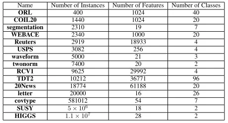
Table 1: Dataset Description

method becomesO(ndD+nbd)whent= 1andO(nubD)

otherwise. The additional memory is reduced fromO(n2₎_to

O(nD), whereDis the number of Fourier components. We empirically setD= 100in our experiment.

Experimental Results

DatasetsWe use fifteen benchmark datasets, seven of which are from UCI machine learning repository (Dheeru and Karra Taniskidou 2017), namely segmentation,waveform,

twonorm,HIGGS,covtype,SUSYandletter. The other eight

datasets areReuters,RCV1,TDT2,20News,WEBACE,ORL,

COIL20andUSPS, which are publicly available2. The tasks

of these datasets range from hand writing digits recognition, object recognition, to text classification. Table 1 summarizes the details of the datasets.

Experiment Setup

All the compared methods are described below.

• LBC: our BMAL method in Algorithm 2.

• LBCdirect: which is a degenerated version of our method

by taking the direct approach.

• LBCscreen: which is another degenerated version of our

method by taking the screening approach.

• Batchrank: the BMAL method proposed in (Chakraborty et al. 2015b) which directly combines mutual information with entropy.

• RPE: the representative BMAL method described in (Wang et al. 2015) using relative Pearson divergence.

• MMD: the QP-based MMD method (Chattopadhyay et al. 2012), which selects samples using QP relaxation.

• MCDR: the BMAL method in (Wang and Ye 2015) which directly combines MMD with a regression loss

• Rand: random selection, which selects b samples uni-formly at random.

In the experiment, we randomly split each dataset into unlabeled data (60%) and testing data (40%). One instance from each class is randomly selected as the initial labeled

2

(7)

Time(s) acc.ratio

Dataset MMD RPE Batchrank MCDR LBC vs. MMD vs. RPE vs. Batchrank vs. MCDR

ORL 0.35 0.21 0.28 2.81 0.01 63.88 38.38 51.41 513.30

COIL20 37.84 19.37 8.70 59.52 0.16 234.97 120.28 54.04 369.58

segmentation 240.34 82.02 13.06 165.93 0.46 523.09 178.52 28.43 361.14

WEBACE 188.12 77.48 25.81 158.67 0.49 387.41 159.56 53.14 326.77

Reuters 539.71 99.73 16.76 384.22 0.83 647.73 119.69 20.12 461.12

USPS 368.49 133.81 19.83 147.28 0.89 414.07 150.37 22.29 165.50

waveform 3131.24 345.51 42.55 204.78 2.51 1245.58 137.44 16.93 81.46

twonorm 78.35 737.10 73.81 191.39 5.68 13.80 129.85 13.00 33.72

RCV1 7458.11 1061.75 184.23 11320.09 9.66 772.08 109.91 19.07 1171.88

TDT2 71093.94 239270.75 3567.2 5251.77 195.31 364.01 1225.05 18.26 26.89

20News NA NA 12951.53 NA 333.45 33.84

letter NA NA 25325.87 NA 598.61 42.31

covtype MLE MLE MLE MLE 10296.35

SUSY MLE MLE MLE MLE 59595.7

HIGGS MLE MLE MLE MLE 159035.40

Table 2: Total running time (in seconds) of five compared methods along with accelerating ratio ofLBCagainst the other four. NA represents the method fails to provide with a result after running for several days, and MLE indicates that the method runs out of memory.

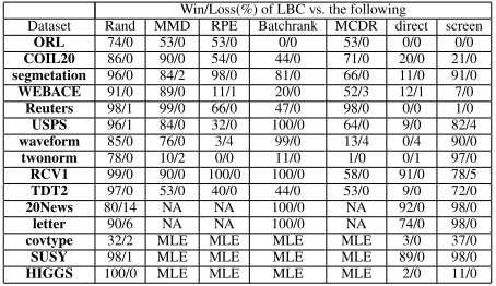
Win/Loss(%) of LBC vs. the following

Dataset Rand MMD RPE Batchrank MCDR direct screen

ORL 74/0 53/0 53/0 0/0 53/0 0/0 0/0 COIL20 86/0 90/0 54/0 44/0 71/0 20/0 21/0 segmetation 96/0 84/2 98/0 81/0 66/0 11/0 91/0 WEBACE 91/0 89/0 11/1 20/0 52/3 12/1 7/0

Reuters 98/1 99/0 66/0 47/0 98/0 0/0 1/0

USPS 96/1 84/0 32/0 100/0 64/0 9/0 82/4

waveform 85/0 76/0 3/4 99/0 13/4 0/4 90/0 twonorm 78/0 10/2 0/0 11/0 1/0 0/1 97/0

RCV1 99/0 90/0 100/0 100/0 58/0 91/0 78/5

TDT2 97/0 53/0 40/0 44/0 53/0 9/0 72/0 20News 80/14 NA NA 100/0 NA 92/0 98/0 letter 90/6 NA NA 100/0 NA 74/0 98/0 covtype 32/2 MLE MLE MLE MLE 3/0 37/0 SUSY 98/1 MLE MLE MLE MLE 89/0 98/0 HIGGS 100/0 MLE MLE MLE MLE 2/0 11/0

Table 3: the win/loss(%) ofLBC against BMAL baselines using paired t-test with a 95% significant level

data. All methods are applied with the same initial, unla-beled and testing dataset. The batch sizebis fixed to be100

on large datasetscovtype,SUSY andHIGGS,50 onletter

and20News, and10 on other small datasets. Logistic

Re-gression is used as the classifier. For each dataset, the exper-iment is conducted 10 times. The averaged result is reported. We use Gaussian kernel on all datasets. For data instances

xandywe setK(x,y) =exp(−||x−y||2_/p)_{, where the}

parameterpis themedianof all pair-wise squared Euclidean distances over the unlabeled data. We sort all the unlabeled samples increasingly according to their certainty in Eq. (10), and set hyper-parameterto be theβ-th percentile (0< β < 100). We empirically use two hyper-parameter γ andτ to describeβas β =γ∗(nu/n)τ_{, where}_γ_and_τ _{is fixed to}

be 20 and10 respectively. For hyper-parameter λ, we set

λ=b2_{. The two degenerated methods use the same}

hyper-parameters as our method. For the three largest datasets, we use the memory-efficient version of Algorithm 2 instead.

Experimental Results

Running Time.Table 2 shows the total running time of five

compared methods, along with the accelerating ratio ofLBC

against the other four. For datasets such as20Newsand let-ter, some baselines are omitted because they cannot present the results after running several days. For datasetscovtype,

HIGGSandSUSY, where the number of unlabeled instances

reaches105 to 106, four baselines run out of memory. As can be seen, LBChas smaller running time on all datasets against the four complex baselines. It is interesting to in-vestigate the accelerating ratio ofLBC againstMMDsince they are solving similar objective using different solvers. For datasetsRCV1,LBCis over 700 times faster thanMMD, and for datasetwaveform, the accelerating ratio is over 1200.

Accuracy.Figure 1 shows the average accuracy of all com-pared methods over fifteen datasets. We can see that our algorithm at least does not lose accuracy from the figures. Table 3 further reveals the percentage of win/loss of LBC

against five baselines using paired t-test withp <0.05. The t-tests are conducted on the accuracy of compared meth-ods over 10 runs. As we can see, LBC wins most of the batches on most datasets. Our method ties againstRPE on dataset twonorm, and also ties against batchrank onORL. It also becomes slightly worse in accuracy on dataset

wave-formandtwonormagainstLBCdirect. InReutersandORL,

the two degenerated versions have similar performance with our method.

Conclusion

(8)

Acknowledgments

This work is supported in part by China National 973 pro-gram 2014CB340301.

References

Buchbinder, N.; Feldman, M.; Naor, J. S.; and Schwartz, R. 2014. Submodular maximization with cardinal-ity constraints. In Proceedings of the Twenty-Fifth

An-nual ACM-SIAM Symposium on Discrete Algorithms, 1433–

1452. SIAM.

Chakraborty, S.; Balasubramanian, V.; Sankar, A. R.; Pan-chanathan, S.; and Ye, J. 2015a. Batchrank: A novel batch mode active learning framework for hierarchical classifica-tion. InProceedings of the 21th ACM SIGKDD Interna-tional Conference on Knowledge Discovery and Data Min-ing. ACM.

Chakraborty, S.; Nallure Balasubramanian, V.; Sun, Q.; Pan-chanathan, S.; and Ye, J. 2015b. Active batch selection via convex relaxations with guaranteed solution bounds. IEEE Transactions on Pattern Analysis and Machine Intelligence

37(10):1945 – 1958.

Chattopadhyay, R.; Wang, Z.; Fan, W.; Davidson, I.; Pan-chanathan, S.; and Ye, J. 2012. Batch mode active sampling based on marginal probability distribution matching. In Pro-ceedings of the 18th ACM SIGKDD International

Confer-ence on Knowledge Discovery and Data Mining, 741–749.

Chen, Y., and Krause, A. 2013. Near-optimal batch mode active learning and adaptive submodular optimization. In

Proceedings of the 30th International Conference on

Ma-chine Learning, 160–168.

Cheng, Y.; Chen, Z.; Fei, H.; Wang, F.; and Choudhary, A. N. 2014. Batch mode active learning with hierarchical-structured embedded variance. InSIAM International

Con-ference on Data Mining, 10–18. SIAM.

Chitta, R.; Jin, R.; and Jain, A. K. 2012. Efficient kernel clustering using random fourier features. In2012 IEEE 12th

International Conference on Data Mining, 161–170. IEEE.

Dheeru, D., and Karra Taniskidou, E. 2017. UCI machine learning repository.

Gretton, A.; Borgwardt, K. M.; Rasch, M.; Sch¨olkopf, B.; and Smola, A. J. 2006. A kernel method for the two-sample-problem. In Advances in Neural Information Processing

Systems, 513–520.

Gretton, A.; Borgwardt, K. M.; Rasch, M. J.; Sch¨olkopf, B.; and Smola, A. 2012. A kernel two-sample test.The Journal

of Machine Learning Research13(1):723–773.

Gu, Q.; Zhang, T.; and Han, J. 2014. Batch-mode active learning via error bound minimization. InProceedings of the

30th Conference on Uncertainty in Artificial Intelligence,

300–309.

Guo, Y., and Schuurmans, D. 2008. Discriminative batch mode active learning. InAdvances in Neural Information

Processing Systems, 593–600.

Guo, Y. 2010. Active instance sampling via matrix par-tition. InAdvances in Neural Information Processing Sys-tems, 802–810.

Hoi, S. C.; Jin, R.; Zhu, J.; and Lyu, M. R. 2006. Batch mode active learning and its application to medical image classifi-cation. InProceedings of the 23rd International Conference

on Machine Learning, 417–424.

Reyes, O., and Ventura, S. 2018. Evolutionary strategy to perform batch-mode active learning on multi-label data.

ACM Transactions on Intelligent Systems and Technology

(TIST)9(4):46.

Scheffer, T.; Decomain, C.; and Wrobel, S. 2001. Active hidden markov models for information extraction. In

Inter-national Symposium on Intelligent Data Analysis, 309–318.

Springer.

Settles, B. 2010. Active learning literature survey.

Univer-sity of Wisconsin, Madison52:55–66.

Seung, H. S.; Opper, M.; and Sompolinsky, H. 1992. Query by committee. InProceedings of the 5th annual workshop

on Computational learning theory, 287–294. ACM.

Tong, S., and Koller, D. 2002. Support vector machine active learning with applications to text classification.The Journal

of Machine Learning Research2:45–66.

Wang, Z., and Ye, J. 2015. Querying discriminative and representative samples for batch mode active learning.ACM

Transactions on Knowledge Discovery from Data9(3):17:1–

17:23.

Wang, H.; Du, L.; Zhou, P.; Shi, L.; and Shen, Y.-D. 2015. Convex batch mode active sampling viaα-relative pearson divergence. InProceedings of the 29th AAAI Conference on

Artificial Intelligence.

Wang, H.; Chang, X.; Shi, L.; Yang, Y.; and Shen, Y.-D. 2018. Uncertainty sampling for action recognition via max-imizing expected average precision. InProceedings of the Twenty-Seventh International Joint Conference on Artificial

Intelligence, 964–970.

Wei, K.; Iyer, R.; and Bilmes, J. 2015. Submodularity in data subset selection and active learning. In Proceedings

of the 32nd International Conference on Machine Learning,

1954–1963.

Yan, Y., and Huang, S.-J. 2018. Cost-effective active learn-ing for hierarchical multi-label classification. In Proceed-ings of the Twenty-Seventh International Joint Conference

on Artificial Intelligence, 2962–2968.

Yang, Y.; Ma, Z.; Nie, F.; Chang, X.; and Hauptmann, A. G. 2015. Multi-class active learning by uncertainty sampling with diversity maximization.International Journal of