Differential Privacy for Bayesian Inference through Posterior
Sampling
∗Christos Dimitrakakis [email protected] University of Lille, F-59650 Villeneuve-d’Ascq, France
SEAS, Harvard University, Cambridge MA-02138, USA
DIT, Chalmers University of Technology, SE-412 96, Gothenburg, Sweden
Blaine Nelson [email protected]
Google, Inc.
1600 Amphitheatre Parkway Mountain View, CA 94043, USA
Zuhe Zhang [email protected]
School of Mathematics & Statistics The University of Melbourne Parkville, VIC 3010, Australia
Aikaterini Mitrokotsa [email protected]
Department of Computer Science & Engineering Chalmers University of Technology
SE-412 96, Gothenburg, Sweden
Benjamin I. P. Rubinstein [email protected] School of Computing & Information Systems
The University of Melbourne Parkville, VIC 3010, Australia
Editor:Charles Elkan
Abstract
Differential privacy formalises privacy-preserving mechanisms that provide access to a database. Can Bayesian inference be used directly to provide private access to data? The answer is yes: under certain conditions on the prior, sampling from the posterior dis-tribution can lead to a desired level of privacy and utility. For a uniform treatment, we define differential privacy over arbitrary data set metrics, outcome spaces and distribution families. This allows us to also deal with non-i.i.d or non-tabular data sets. We then prove bounds on the sensitivity of the posterior to the data, which delivers a measure of robustness. We also show how to use posterior sampling to provide differentially private responses to queries, within a decision-theoretic framework. Finally, we provide bounds on the utility of answers to queries and on the ability of an adversary to distinguish between data sets. The latter are complemented by a novel use of Le Cam’s method to obtain lower bounds on distinguishability. Our results hold for arbitrary metrics, including those for the common definition of differential privacy. For specific choices of the metric, we give a number of examples satisfying our assumptions.
∗. A preliminary version of this paper appeared inAlgorithmic Learning Theory 2014(Dimitrakakis et al., 2014). This version corrects proofs, constant factors in the upper bounds and introduces new material on utility analysis, lower bounds and examples.
c
Keywords: Bayesian inference, differential privacy, robustness, adversarial Learning
1. Introduction
The Bayesian framework for statistical decision theory incorporates uncertainty into decision making in a probabilistic manner. This makes the framework attractive, as predictions and modelling can all be made with the machinery of probability. More specifically, a Bayesian statistician begins by assuming that the world is described by a probabilistic model within some family, and he assigns a prior belief to each one of the models. After observing data, this belief is adjusted through Bayes’s theorem to the so called posterior belief. This expresses the statistician’s conclusion given the data and the prior assumptions. The statistician can then release the posterior to the world, for others to build upon, or use for principled decision making under uncertainty.
Unfortunately, it is frequently the case that the data acquired by the statistician is sensitive. Consequently, there is a fear that any information released by the statistician that depends on the data—be that the posterior distribution itself or any decisions that follow from the calculated posterior—may reveal sensitive information in the original data. Recently, the framework of differential privacy has been proposed to codify this leakage of information. If an algorithm is differentially private, then its output can only leak a bounded amount of information about its input.
We are interested in the question of how one can build differentially-private algorithms within the Bayesian framework. More precisely, we examine when the choice of prior is sufficient to guarantee differential privacy for decisions that are derived from the posterior distribution. Our work develops a unified understanding of privacy and learning in adver-sarial environments, under a decision-theoretic framework. We show that under suitable assumptions, standard Bayesian inference and posterior sampling can achieve uniformly good utility with a fixed privacy budget in the differential privacy setting. We also indicate strong connections between robustness and privacy. Under the base level of data privacy provided by the posterior distribution, the statistician can safely respond to external queries using samples from the posterior. When estimating a linear model from sensitive data, for example, samples from the posterior correspond to different possible fits. The more samples used, the more privacy is leaked, while query responses may be more accurate.
Our proposed approach complements existing mechanisms rather well, and may be par-ticularly useful in situations where Bayesian inference is already in use. For this reason, we provide illustrative examples in the exponential family. However, our setting is wholly general and not limited to specific distribution families, or i.i.d. observations. Any family could be chosen: so long as it either satisfies our assumptions directly, or can be restricted so that it does. For example, our framework applies to families of discrete Bayesian net-works with directed-acyclic topologies (e.g., Markov chains; see Lemma 24 on page 21) and multivariate Gaussians (see Lemma 23), where the observations may not satisfy the i.i.d. assumption.
1. B selects a model family (FΘ) and a prior (ξ).
2. A is allowed to seeFΘ and ξ and is computationally unbounded.
3. B observes datax and calculates the posteriorξ(θ|x) but does not reveal it. Then, for stepst= 1,2, . . ., repeat the following:
4. A sends his utility function u and a queryqt toB.
5. B responds with the response rt maximising u, in a manner that depends on the query and the posterior.
Let us now elaborate. In this framework, the choice of the model familyFΘis dictated by the problem. The choice ofξis normally determined by the prior knowledge ofB, but we show that this also affects what level of privacy is achieved. Informally speaking, informative priors achieve better privacy, as the posterior has a weaker dependency on the data. It is natural to assume that the prior itself is public, as it should reflect publicly available information. The statistician’s conclusion from the observed datax is then summarised in the posterior distributionξ(θ|x), which remains private.
The second part of the process is the interaction withA. We adopt a decision-theoretic viewpoint to characterise what the optimal responses to queries should be. More specifically, we assume the existence of a “true” parameter θ ∈ Θ, and that A has a utility function
uθ(qt, rt), which he wishes to maximise. For example, consider the case where θ = (µ, Σ) are the parameters of a normal distribution. An example query qt is “what is the expected
value Eθxi =µof the distribution?”. The optimal responsert, would then be a real vector that depends on the utility function. A possible utility function is the negative squared L2
distance:
uθ(qt= “what is the mean?”, rt) =−kEθxi−rtk22.
While θ is unknown, B has information about it in the form of a posterior distribution. Using standard decision-theoretic notions, the optimal response of B would maximise the expected utilityEξ(u|qt, rt, x), where the expectation is taken over the posterior distribu-tion. However, this deterministic response cannot be differentially private.
In this paper, we promote the use of posterior sampling to respond to queries. The posterior sampling mechanism draws a set ˆΘof i.i.d. samples from the posterior distribution. Then, all the responses only depend on the posterior through ˆΘ. Since our algorithm only takes a single sample set ˆΘ, further queries by the adversary reveal nothing more about the data than what can be inferred from ˆΘ. The empirical distribution induced by ˆΘ serves as a private surrogate for the exact (non-private) posterior. Consequently, we can respond to an arbitrary number of queries with a bounded privacy budget, while guaranteeing good utility for all responses.
We show that if FΘ and ξ are chosen appropriately, this results in differentially-private responses, as well as robustness of the posterior.1 In addition, we prove upper and lower
bounds on how easy it is for an adversary to distinguish two -close data sets. Finally, we bound the loss in utility incurred due to privacy. The intuition behind our results
is that robustness and privacy are linked via smoothness. Learning algorithms that are smooth mappings—their output (e.g., a spam filter) varies little with perturbations to input (e.g., similar training corpora)—are robust: outliers have reduced influence, and adversaries cannot easily discover unknown information about the data. This suggests that robustness and privacy can be simultaneously achieved and are in fact deeply linked.
We provide a uniform mathematical treatment of the privacy and robustness properties of Bayesian inference based on generalised differential privacy to arbitrary data set distances, outcome spaces, and distribution families. This paper can be summarised as making the following distinct contributions:
• Under certain regularity conditions on the prior distribution ξ or likelihood family
FΘ, we show that the posterior distribution is robust: small changes in the data set result in small posterior changes.
• We introduce a novel posterior sampling mechanism that is private.2 Unlike other common mechanisms in differential privacy, our approach sits squarely in the non-private (Bayesian) learning framework without modification.
• We provide necessary and sufficient conditions for differentially private Bayesian in-ference.
• We introduce the notion of data set distinguishability for which we provide finite-sample bounds for our mechanism: how large would ˆΘ need to be forA to distinguish two data sets with high probability.
• We provide examples of conjugate-pair distributions where our assumptions hold, including discrete Bayesian networks. We find that even though Bayesian posterior sampling does provide privacy guarantees directly, those appear to be very weak for standard conjugate families. However, with a small modification of the prior, it is easy to obtain good privacy guarantees.
Paper organisation. Section 2 specifies the setting and our assumptions. Section 3 proves results on robustness of Bayesian learning. Section 4 proves our main privacy results. In particular, Section 4.1 shows that the posterior distribution is differentially private, Section 4.2 describes our posterior sampling query response algorithm, Section 4.3 derives bounds on data set indistinguishability, Section 4.5 shows how to obtain matching lower bounds for distinguishability, while Section 4.4 shows how utility and privacy can be traded off within our framework. Examples where our assumptions hold are given in Section 5. We present a discussion of our results, related work and links to the exponential mechanism and robust Bayesian inference in Section 6. Appendix A contains proofs of the main theorems. Finally, Appendix B details proofs of the examples demonstrating our assumptions.
2. Problem Setting
We consider the problem of a Bayesian statistician (B) communicating with an untrusted third party (A). B wants to convey useful responses to the queries of A (e.g., how
many people suffer from a disease or vote for a particular party) without revealing private information about the original data (e.g., whether a particular person has cancer). This requires communicating information in a way that strikes a balance between utility and privacy. In this paper, we study the inherent privacy and robustness properties of Bayesian inference and explore the question of whether B can select a prior distribution so that a computationally unbounded A cannot obtain private information from queries.
2.1 Definitions and Notation
We begin with our notation. LetS be the set of all possible data sets. For example, ifX is a finite alphabet, then we might haveS =S∞
n=0Xn,i.e., the set of all possible observation
sequences over X. However, S can have arbitrary structure and so social network or mo-bility trace data are also handled in this framework. Probamo-bility measures on parameters
θ are usually denoted by ξ, while measures and densities on data are denoted by Pθ or pθ respectively. Expectations are denoted byEξg,
R
Θg(θ) dξ(θ), where the subscript denotes the underlying distribution with respect to which we are taking expectations. In case of ambiguity, we explicitly write e.g., Ex∼Pθf(x) =
R
Sf(x) dPθ(x) to denote which variables
are drawn from which distributions. Finally, we useI{π}to be the identity function, taking
the value 1 when the predicateπ is true, and 0 otherwise.
2.1.1 Distances Between Data Sets
Central to the notions of privacy and robustness, is the concept of distance between data sets. Firstly, the effect of data set perturbation on learning depends on the amount of noise as quantified by some distance. This is useful for characterising robustness to noise or adversarial manipulation of the data. Secondly, the amount that an attacker can learn from queries can be quantified in terms of the distance of his guesses to the true data set. Finally, it allows for a unified mathematical treatment, as it permits different types of neighbourhoods to be defined. To model these situations, we equip S with a pseudo-metric3 ρ :S × S → R+. This generalisation has also been used by Chatzikokolakis et al. (2013), which has laid the groundwork for metric-based differential privacy. While this concept has many applications in the context of geographical information systems, we apply this generalisation of differential privacy without necessarily referring to some underlying physical distance.
2.1.2 Bayesian Inference
This paper focuses on theBayesian inferencesetting, where the statistician Bconstructs a posterior distribution from a prior distributionξ and a training data setx. More precisely, we assume that datax∈ Shave been drawn from some distributionPθ? onS, parameterised
byθ?, from a family of distributionsFΘ. B defines a parameter setΘ indexing a family of distributions FΘ on (S,SS), where SS is an appropriateσ-algebra on S:
FΘ,{Pθ:θ∈Θ},
and where we use pθ to denote the corresponding densities4 when necessary. To perform inference in the Bayesian setting, B selects a prior measure ξ on (Θ,SΘ) reflecting B’s subjective beliefs about whichθis more likely to be true,a priori;i.e., for any measurable set
B ∈SΘ,ξ(B) representsB’s prior belief thatθ? ∈B. In general, the posterior distribution after observingx∈ S is:
ξ(B |x) =
R
Bpθ(x) dξ(θ)
φ(x) , (1)
whereφ is the corresponding marginal density given by:
φ(x),
Z
Θ
pθ(x) dξ(θ) .
While the choice of the prior is generally arbitrary, this paper shows that its careful selec-tion can yield good privacy guarantees. Throughout the paper, we shall use the following simple example to ground our observations and theory. This consists of a finite family of distributions, on a finite alphabet. Consequently, calculation of the posterior distribution is always simple. It is also easy to verify our assumptions on this model.
Example 1 (Finite Bernoulli family.) Consider a finite family of distributions FΘ =
{Pθ :θ∈Θ} on alphabetX ={0,1}, with θ∈[0,1], such that for any model in the family
and any observation x
Pθ(x) =θI{x= 1}+ (1−θ)I{x= 0}.
For any sequence of observations x1, . . . , xT, we have, with some abuse of notation,
Pθ(x1, . . . , xT) = T
Y
t=1
Pθ(xt),
i.e., Pθ defines an i.i.d. distribution on the alphabet. This family corresponds to a set of
Bernoulli models. The set of parameters Θ will be chosen to discretise the parameter space of Bernoulli distributions over ∆-sized intervals. For this, the k-th model’s parameter will be θk=∆k, with∆∈(0,1)and k≤1/∆.
For the above family, we can use a uniform prior distribution ξ(θk) = ∆. The posterior distribution is easily calculated, since we need only sum over a finite number of parameters.
2.1.3 Privacy
We now recall the concept of differential privacy (Dwork, 2006). This states that on neigh-bouring data sets, a randomised query response mechanism yields (pointwise) similar dis-tributions. We adopt the view of mechanisms as conditional distributions under which differential privacy can be seen as a measure of smoothness. In our setting, conditional distributions conveniently correspond to posterior distributions. These can also be inter-preted as the distribution of a mechanism that uses posterior sampling, to be introduced in Section 4.2. The precise definition depends on the notion of neighbourhood, with the following choice being common:
Definition 1 ((, δ)-differential privacy) A conditional distributionP(· |x) on(Θ,SΘ)
is (, δ)-differentially private if, for all B ∈SΘ and for any x∈ S =Xn
P(B |x)≤eP(B |y) +δ,
for ally in the Hamming-1 neighbourhoodof x. That is, y may differ in at most one entry from x: there is at most one i∈ {1, . . . , n} such that xi 6=yi.
A typical situation where this definition is employed, is when x, y are matrices andxi is a single row in the matrix. Then, the data sets are neighbours if a matrix row is changed.5
In our setting, it is reasonable to generalise this to arbitrary data set spacesS that are not necessarily product spaces. To do so, we use the notion of differential privacy under a pseudo-metric ρ on the space of all data sets, which allows for more subtle representations of attacker knowledge and for a more general treatment:
Definition 2 ((, δ)-differential privacy under ρ.) A conditional distribution P(· | x)
on (Θ,SΘ) is (, δ)-differentially private under a pseudo-metric ρ:S × S →R+ if, for all
B ∈SΘ and for any x, y∈ S,
P(B|x)≤eρ(x,y)P(B |y) +δρ(x, y).
In our setting,ρ replaces the notion of neighbourhood. It is of course possible to useρthat corresponds to the usual meaning of neighbourhood in differential privacy:
Remark 3 If S = Xn and ρ(x, y) = Pn
i=1I{xi 6=yi} is the Hamming distance, this def-inition is analogous to standard (, δ)-differential privacy. When considering only (,0) -differential privacy or (0, δ)-privacy, it is an equivalent notion.6
Proof For (,0)-DP, let ρ(x, z) =ρ(z, y) = 1; i.e., the data differ in one element. Then, from standard DP, we have P(B | x) ≤ eP(B | z) and so obtain P(B | x) ≤ e2P(B |
y) =eρ(x,y)P(B |y). By induction, this holds for anyx, y pair. Similarly, for (0, δ)-DP, by induction we obtain P(B |x)≤P(B |y) +δρ(x, y).
Definition 1 allows for privacy against a powerful attackerA, who attempts to match the empirical distribution induced by the true data set, by querying the learned mechanism and comparing its responses to those given by distributions simulated using knowledge of the mechanism and knowledge of all but one datum—narrowing the data set down to a Hamming-1 ball. Indeed the requirement of differential privacy is sometimes too strong
since it may come at the price of utility. Definition 2 allows for a much broader encoding of the attacker’s knowledge via the selected pseudo-metric. It also allows a more fine-grained notion of privacy. This is quite useful for geographical information systems, as proposed by Chatzikokolakis et al. (2013), to which we refer the reader for a broader discussion of the use of metrics in differential privacy.
Finally, we can show that this generalisation of differential privacy satisfies the standard composition property.
5. Another common choice for neighbourhoods is to say that two data sets are neighbours if one results from the other by addition of a row.
Theorem 4 (Composition) Let conditional distributions P(· | x) on (Θ,SΘ) be (, δ )-differentially private under a pseudo-metric ρ:S × S → R+ and P0(· |x) on (Θ0,S0Θ0) be
(0, δ0)-differentially private underthe same pseudo-metric. Then the conditional distribution on the product space (Θ×Θ0,SΘ⊗S0Θ0) given by
Q(B×B0 |x) =P(B |x)P0(B0 |x),∀B×B0 ∈SΘ⊗S0Θ0
satisfies (+0, δ+δ0)-differentially private under the pseudo-metric ρ. Here SΘ⊗S0Θ0 is
the product σ-algebra on Θ×Θ0.
Proof For any y∈ S
Q(B×B0 |x)≤heρ(x,y)P(B |y) +δρ(x, y)iP0(B0 |x)
≤eρ(x,y)P(B |y)
h
e0ρ(x,y)P0(B0 |y) +δ0ρ(x, y)
i
+δρ(x, y)
≤e(+0)ρ(x,y)P(B |y)P0(B0 |y) + (δ+δ0)ρ(x, y)
2.2 Our Main Assumptions
In the sequel, we show that if the distribution familyFΘ or priorξsatisfies certain assump-tions, then close data setsx, y ∈ S result in posterior distributions that are close. In that case, it is difficult for a third party to use such a posterior to distinguish the true data set
x from similar data sets.
To formalise these notions, we introduce two possible assumptions one could make on the smoothness of the familyFΘwith respect to some metricdonR+. The first assumption states that the likelihood is smooth for all parameterisations of the family. First, we define our notion of smoothness. Let f(x, θ),lnpθ(x) be the log probability ofx underθ. The Lipschitz constant for a parameter valueθ is:
`(θ),inf{u:|f(x, θ)−f(y, θ)| ≤uρ(x, y)∀x, y∈ S }. (2)
Our first assumption is uniform smoothness for all parameters.
Assumption 1 (Lipschitz continuity) We assume there exists some L <∞ such that:
`(θ)≤L, θ∈Θ. (3)
In other words, this assumption says that the log probability is Lipschitz with respect to
ρ for any parameter value. Consider Example 1 for the Bernoulli model. It is easy to see that a model with∆-sized intervals satisfies the above assumption withL= ln 1/∆.
0 0.2 0.4 0.6 0.8 1
0 0.5 1 1.5 2 2.5 3
ξ
(
ΘL
)
L
(a) Uniform prior
0 0.2 0.4 0.6 0.8 1
0 0.5 1 1.5 2 2.5 3
L
0.2 cdf 0.05 cdf 0.2 bound 0.05 bound
L(0.2)
L(0.05)
(b) Exponential prior
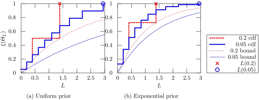
Figure 1: The mass of L-Lipschitz parameters, for two finite familes of Bernoulli distribu-tions with ∆∈ {0.2,0.05} (thick lines) together with their respective stochastic Lipschitz bounds (thin lines) and the corresponding uniform Lipschitz constantL.
sequence containing a 1 has probability 0. The same thing occurs when we take ∆→ 0 in Example 1. To avoid such problems, we relax the assumption by only requiring that B’s
prior probability ξ is concentrated in the regions of the family for which the likelihood is smoothest:
Assumption 2 (Stochastic Lipschitz continuity; Norkin, 1986) First, define the sub-set of parameter values
ΘL ,{θ∈Θ :`(θ)≤L} (4)
to be those parameters for which Lipschitz continuity holds with Lipschitz constantL. Then, there are some constants c, L0>0 such that, for all L≥L0:
ξ(ΘL)≥1−exp(−c(L−L0)) . (5)
By not requiring uniform smoothness, this weaker assumption is easier to meet but still yields useful guarantees. In fact, in Section 5, we demonstrate that this assumption is satisfied by many important example distribution families. However, it will be illustrative to consider the discrete Bernoulli family example at this point.
Example 2 (Continuation of Example 1) These conditions can be examined in terms of the finite family of Example 1. Figure 1 demonstrates the assumptions for ∆= 0.2 (red dashed lines) and ∆= 0.05 (blue solid lines).
In particular, the two thick lines Figure 1a show the probability mass of L-Lipschitz parameters for the two families. They are both step functions, as the families are discrete.7
The × and ◦ symbols show the corresponding Lipschitz constants for the two families re-spectively, and we can clearly see∆= 0.2has about half the Lipschitz constant of∆= 0.05. The thinner curves depict the highest lower bound on the probability mass defined in As-sumption 2. There we see that the higher curve is achieved by∆= 0.2.
In order to improve the lower bound, we need to modify our prior distribution on the family members so as to place less mass on the more sensitive parameters. The result of this operation is shown in Figure 1b, which uses the prior ξ(θ)∝exp(−`(θ)), i.e., it places exponentially smaller weight in more sensitive parameters. This results in both lower bounds being shifted upwards, corresponding to a higher c constant in Assumption 2. Of course, this has no effect on Assumption 1.
For completeness, we now show that verifying our assumptions for a distribution of a single random variable lifts to a corresponding property for the product distribution on i.i.d. samples.
Lemma 5 IfFΘsatisfies Assumption 1 (resp. Assumption 2) with respect to pseudo-metric
ρ and constant L (or c), then, for any fixed n∈ N, the product family Fn
Θ with densities
(sim. measures) pnΘ({xi}) =Qni=1pΘ(xi) satisfies the same assumption with respect to:
ρn({xi},{yi}) =
Pn
i=1ρ(xi, yi)
and constant L (or c).
2.2.1 Necessary Conditions
Finally, let us discuss whether the above conditions are necessary to achieve differential privacy. In fact, either the first condition must be true, or a similar condition must hold on the marginals for every possible data set pair (x, y). Our second condition can be seen as a specific case of the necessary condition for the marginals, as explained below.
Theorem 6 For a prior ξ to be 2L-differentially private for a family FΘ, either
sup θ∈Θ
lnPθ(x)
Pθ(y) ≤Lρ(x, y), or ln
φ(y)
φ(x) ≤Lρ(x, y) (6)
for all x, y∈ X.
Proof If neither condition holds for some pair (x, y) then there is θ such that lnPPθ(θ(xy)) > Lρ(x, y) and lnφφ((yx)) > Lρ(x, y). Simply adding the two, we obtain lnξξ((θθ||xy)) >2Lρ(x, y), and so the resulting posterior is notL-differentially private.
In our main results, we show that the first part of the conditions, which is equivalent to our first assumption, is also sufficient. However, the second part is too weak to imply differential privacy on its own.
2.2.2 The Choice of Metric and Sufficient Statistics
The extent to which our assumptions hold for a particular family of distributionsFΘdepends mainly onρ.8 The choice of metric is also important for achieving differential privacy with
respect to it. Let us specifically consider metrics defined in terms of a difference in statistics:
ρ(x, y),kτ(x)−τ(y)k ,
whereτ :S → V is a statistic mapping from data sets to a normed vector space.
In that case, our assumptions imply thatτ must be asufficient statistic, since ifτ(x) =
τ(y) then ρ(x, y) = 0 and it follows that Pθ(x) = Pθ(y). More generally, ρ must be such that if the distance between x, y is zero, then their probabilities should be equal. We will see some examples of such statistics for conjugate distributions in the exponential family in Section 5. That means that we cannot use a metric which simply ignores part of the data, for example.
Similarly, the very definition of differential privacy (Definition 2) implies that τ must be a Bayes-sufficient statistic. That means that for any x, y, it holds
τ(x) =τ(y) ⇒ ξ(B |x) =ξ(B|y), ∀B ∈SΘ.
Note that this is a slightly weaker condition than a sufficient statistic, which is necessary for our assumptions to hold.
2.3 Summary of Results
Given the above assumptions, we show: firstly, that if we choose an informative prior ξ, the resulting posterior is robust in terms of KL-divergence to small changes in the data. Secondly, that the posterior distribution is differentially private. Thirdly, that this implies that sampling from the posterior can be used as part of a differentially-private mechanism. We complement these with results on how easily an adversary can distinguish two similar data sets from posterior samples. Finally, we characterise the trade-off between utility and privacy, stated here informally for ease of exposition:
Claim 1 IfA prefers to use the priorξ?, butBuses a priorξsatisfying Assumption 1, and
A’s utility is bounded in [0,1], the following is true for the posterior sampling mechanism with N samples:
• The mechanism is2N L-differentially private.
• A’s utility loss isO[1−ξ?(Θ L)] +
p
1/N w.h.p., where ΘL is the support ofξ.
The following sections discuss our main results in detail. We begin by proving that our assumptions result in robust posteriors, in the sense that the KL divergence between posteriors arising from similar data sets is small. Then we show that they also result in differentially private posterior distributions, and analyse the resulting posterior sampling mechanism. We conclude with some examples and a discussion of related work.
3. Robustness of the Posterior Distribution
the case where we measure the distance between the posteriors in terms of the well-known KL-divergence:
D(P kQ) =
Z
S ln dP
dQdP .
The following theorem shows that any distribution family FΘ and prior ξ satisfying one of our assumptions is robust, in the sense that the posterior does not change significantly with small changes to the data set. It is notable that our mechanisms are simply tuned through the choice of prior.
Theorem 7 When ξ is a prior distribution onΘ andξ(· |x)and ξ(· |y)are the respective posterior distributions for data sets x, y∈ S, the following results hold:
1. Under a pseudo-metric ρ and L >0 satisfying Assumption 1,
D(ξ(· |x) k ξ(· |y))≤2Lρ(x, y) . (7)
2. Under a pseudo-metric ρ and c >1 satisfying Assumption 2,
D(ξ(· |x) k ξ(· |y))≤CFΘ
ξ 1 + 2L0+c−1
ρ(x, y) , (8)
where CFΘ
ξ is the ratio between the maximum and marginal likelihoods (9), and
as-suming there exists χ∈(0,1] such that: ∀x, y∈ S there is a sequence {zk} ⊂ S, with
z0=x, zn=y, satisfyingχρ(zk, zk+1)≤c−1 ∀zk.
Note that the second claim bounds the KL divergence in terms of B’s prior belief that
L is small, which is expressed via the constant c. The larger c is, the less prior mass is placed in large L and so the more robust inference becomes. Of course, choosing c to be too large may decrease efficiency.
It is important to also discuss the constantCFΘ
ξ . To get a better intuition, consider the case where Θ,X are finite. Let θ?ML(x) be the maximum-likelihood estimate for x. Then we have that:
CFΘ
ξ = maxx
Pθ?
ML(x)(x)
P
ΘPθ(x)ξ(θ)
≤ max x
1
ξ(θ?
ML(x))
, (9)
there is therefore a natural dependency on the prior mass placed on maximum-likelihood estimators.
Finally,χis going to be 1 for most metric spaces of interest. A notable exception is when the Hamming distance is used, which requires χ < 1 as an additional technical condition forc <2. However, this only affects our results under the second assumption.
4. Privacy and Utility
interpreted as the differential privacy of aposterior sampling mechanism for responding to queries (described in Section 4.2), for which we prove a bound on the utility depending on the number of samples taken. Section 4.3 examines an alternative notion of privacy, data set distinguishability, similar to Wasserman and Zhou (2010). For this, we prove a bound on privacy, that also depends on the number of samples taken. Together, these exhibit a trade off between utility and privacy controlled by choosing the number of samples appropriately, in a manner described in Section 4.4.
4.1 Differential Privacy of Posterior Distributions
We consider our generalised notion of differential privacy for posterior distributions (Defi-nition 2); and show that the type of differential privacy exhibited by the posterior depends on which assumption holds.
Theorem 8 1. Under a pseudo-metric ρ and L > 0 satisfying Assumption 1, for all
x, y∈ S, B ∈SΘ:
ξ(B |x)≤exp{2Lρ(x, y)}ξ(B |y).
i.e., the posteriorξ is (2L,0)-differentially private under pseudo-metric ρ.
2. Under a pseudo-metric ρ and c >1 satisfying Assumption 2, CFΘ
ξ defined in (9), for
allx, y∈ S, B∈SΘ:
|ξ(B |x)−ξ(B |y)| ≤
s
CFΘ
ξ
2 (1 + 2L0+c
−1)ρ(x, y),
i.e., the posterior ξ is0, O(
q
CFΘ
ξ (L0+ 1/c))
-differentially private9 under pseudo-metric √ρ.
The difference between the two bounds’ form is due to the fact that while the first claim has a direct proof, the second claim arises from the KL divergence bound in Theorem 7.
Finally, we show that posterior distributions are also randomly differentially private.
Corollary 9 Under pseudo-metric ρ, c >1 and L≥L0 >0 satisfying Assumption 2: P[∀B ∈SΘ:ξ(B|x)≤exp{2Lρ(x, y)}ξ(B|y),∀x, y∈ S]≥1−exp(−c(L−L0)).
i.e., the posterior ξ is (2L,0,exp(−c(L−L0)))-randomly differentially private (Hall et al., 2011) under pseudo-metric ρ.
This is a conceptually different definition from the original RDP, as the measure over which the randomness is defined is not the data distribution, but the prior measureξ.
This property of the posterior distribution directly leads to the definition of a posterior sampling mechanism which will be differentially private. This is explained in the following section.
4.2 Posterior Sampling Mechanism
Given that we have a full posterior distribution which is differentially private, we can use it to define a private mechanism. We may allow the adversary to submit an arbitrary set of queries {qt} with each qt ∈ Q. Each query warrants a response rt in a set of possible responses R. The adversary is allowed to condition the queries on our previous responses.
We extend our original approach (Dimitrakakis et al., 2014) to take some utility function
uinto account, which scores preferences of responses given a query. The algorithm requires a prior ξ to be defined on a family FΘ of probability distributions, whose members do not necessarily generate i.i.d. observations. They could be Markov chains for example. The first step is to simply draw a number of samples from the posterior, as in the original approach (Algorithm 2). After the algorithm calculates the posterior distributionξ(· |x),N
parameter samples are drawn from it, producing a parameter set ˆΘ. Thereafter, responses depend only on the utility function and the sample ˆΘ, and we do not draw new samples after every query. This allows us to work with a fixed privacy budget.
Algorithm 1 BAPS: Bayesian Posterior Sampling
1: inputpriorξ, datax∈ S
2: Calculate posteriorξ(θ|x).
3: fork= 1, . . . , N do 4: Sampleθ(k) ∼ξ(θ|D).
5: end for
6: return Θˆ =θ(k):k= 1, . . . , N .
Corollary 10 Algorithm 1 is differentially private under the conditions of Theorem 8, namely:
1. Under a pseudo-metricρandL >0satisfying Assumption 1, the algorithm is(2N L,0) -differentially private under pseudo-metric ρ; or
2. Under a pseudo-metric ρ andc >1 satisfying Assumption 2, CFΘ
ξ defined in (9), the
algorithm is 0, O(N
q
CFΘ
ξ (L0+ 1/c))
-differentially private under pseudo-metric
√
ρ.
Proof This follows directly from Theorems 8 and 4 (composition), as the algorithm sam-ples from the posterior distribution, which is differentially private.
Utility and optimal responses. We assume the collection of a set of utility functions
expected utility with respect to the posterior. This corresponds to marginalising outθ, and responding with:
rt ∈ arg max r
Z
Θ
uθ(qt, r) dξ(θ|x) .
The second is to use themaximum a posteriorivalue ofθ. The final, which we employ here, is to use sampling;i.e., to reply to each query using parameters sampled from the posterior. This allows us to reply to arbitrary queries without compromising privacy, since the most information an adversary could obtain is the set of sampled parameters. By adjusting the number of samples used, we can easily trade off between privacy and utility.
After this we respond to a series of queries. For thet-th received queryqt, the algorithm returns the optimal response over the sampled parameter set ˆΘ, in the manner shown in Algorithm 2. Since we allow arbitrary queries, the third party could simply ask for ˆΘ with a suitable choice of the utility function. Then if u is bounded, it is easy to show that the loss due to sampling is bounded.
Algorithm 2 PSAQR: Posterior Sample Query Response
1: inputParameter sample ˆΘ.
2: fort= 1, . . . do
3: Observe query qt∈ Q, perhaps depending onr1, . . . , rt−1 andq1, . . . , qt−1. 4: return rt∈arg maxr
P
θ∈Θˆuθ(qt, r)
5: end for
Lemma 11 The returned responses of the PSAQR mechanism have a utility which is within
O
p
ln(1/δ)/N
of the optimal value with probability at least 1−δ for any δ >0.
Now that we have demonstrated bounds on the utility for the algorithm above, we turn to the issue of how utility and privacy can be optimally tuned. First, we try and quantify the amount of samples an adversary needs to distinguish two data sets.
4.3 Distinguishability of Data Sets
In this section, we wish to relate the size of the sample ˆΘ to the amount of information about x that can be obtained by the adversary A. More precisely, we need to bound how well A can distinguish x from all alternative data sets y. Within the posterior sampling query model,A has to decide whetherB’s posterior isξ(· |x) orξ(· |y). However, he can only do so within some neighbourhoodof the original data. In this section, we boundA’s error in determining the posterior in terms of the number of samples used. This is analogous to the data set-size bounds on queries in interactive models of differential privacy (Dwork et al., 2006), as well as the point of view of privacy as hypothesis testing (Kairouz et al., 2015; Wasserman and Zhou, 2010) where an adversary wishes to distinguish the data set from two alternatives.
Then, the adversary needs only to construct the empirical distribution to approximate the posterior up to some sample error. By bounds on the KL divergence between the empirical and actual distributions we can bound his power in terms of how many samples he needs in order to distinguish betweenx and y.
Due to the sampling model, we first require a finite sample bound on the quality of the empirical distribution. The adversary could attempt to distinguish different posteriors by forming the empirical distribution on any sub-algebra S.
Lemma 12 For any δ ∈ (0,1), let M be a finite partition of the sample space S, of size
m≤log2p1/δ, generating the σ-algebra S=σ(M). Let x1, . . . , xn∼P be i.i.d. samples
from a probability measure P on S, let P|S be the restriction of P onS and let Pˆ|nS be the empirical measure on S. Then, with probability at least1−δ:
Pˆ
n
|S−P|S
1 ≤ r
3
nln
1
δ . (10)
We can combine this bound on the adversary’s estimation error with Theorem 7’s bound on the KL divergence between posteriors resulting from similar data to obtain a measure of how fine a distinction between data sets the adversary can make after a finite number of draws from the posterior:
Theorem 13 Under Assumption 1, the adversary can distinguish between data x, y with probability 1−δ if:
ρ(x, y)≥ 3
4Lnln
1
δ .
Under Assumption 2, this becomes:
ρ(x, y)≥ 3
2n
CFΘ
ξ + 2L0c−1
ln
1
δ .
Consequently, either smoother likelihoods (i.e., decreasing L), or a larger concentration on smoother likelihoods (i.e., increasingc), increases the effort required by the adversary and reduces the sensitivity of the posterior. Note that, unlike the results obtained for differential privacy of the posterior sampling mechanism, these results have the same algebraic form under both assumptions.
4.4 Trading off Utility and Privacy
By construction, in our setting there are three ways with which to tune privacy. The first is the choice of family; the second is the choice of prior; and the third is how many samples
N to draw. The choice of family is usually fixed due to other considerations. However, we have the choice of either tuning the prior, so that we can satisfy our assumptions with some suitable constantsL orc, or by tuning the number of samplesN in the posterior sampling framework.
Lemma 14 If our utility is bounded in [0,1], the private posterior we use is ξ, while the ideal posterior is ξ?, then the regret suffered is bounded by2kξ−ξ?k1.
Finally, consider the case where B, being a true Bayesian, is convinced that ξ? is the correct prior distribution to use, but needs to use the priorξin order to achieve privacy. The following theorem bounds the expected KL divergence between the two resulting posteriors.
Lemma 15 If ∀θ∈Θ, |lnξ?(θ)/ξ(θ)| ≤η then the expected KL divergence is
Ex∼φ?D(ξ?(· |x)kξ(· |x))≤2η ,
where φ? is the ξ? marginal distribution.
We can now combine Lemmas 11 and 14 with Lemma 15, to obtain the following result:
Corollary 16 If A has a preferred prior ξ?, while the private prior used by B is ξ and it satisfies the conditions of Lemma 15, then the loss of A in terms of theξ?-expected utility is Oη+pln(1/δ)/N, with probability at least 1−δ.
Consequently, ifA believes the correct prior should be ξ?, he can use the private posterior sample to make decisions, incurring a small loss. Finally, we already showed thatA cannot distinguish between data that are closer thanO(1/N) with high probability. Hence, in this setting we can tuneN to trade off utility and privacy.
The following theorem characterises the link between the choice of prior, the number of samples, privacy and utility directly. This connects several of our results in one place.
Theorem 17 If, instead of using a non-private prior ξ?, we use a prior ξ restricted on
ΘL (such that it satisfies Assumption 1 with constant L) and generate N samples from the
posterior, then (a) the sample is 2LN-differentially private and (b) the loss of A in terms of the ξ?-expected utility is O[1−ξ?(ΘL)] +
p
ln(1/δ)/N, with probability at least 1−δ
for anyδ >0.
Proof For (a) note that due to composition, N repetitions give 2LN-differential privacy. For (b), letΘLbe the support of ξ. Then, becauseξ is the restriction ofξ? on ΘL, it holds that:
kξ−ξ?k1=ξ(ΘL)−ξ?(ΘL) +ξ?(Θ\ΘL)−ξ(Θ\ΘL) = 2[1−ξ?(ΘL)] .
We now just need to couple this with Lemmas 14 and 11 to directly obtain the stated bound on the utility.
In practice, our choice ofξ gives us a base amount of privacy that depends only onL. By keepingξ fixed and increasing N, we can easily trade off privacy and utility.
4.5 Lower Bounds
It is possible to apply standard minimax theory to obtain lower bounds on the rate of convergence of the adversary’s estimate to the true data. In order to do so, we can for example apply the method due to LeCam (1973), which places lower bounds on the expected distance between an estimator and the true parameter. In order to apply it in our case, we simply replace the parameter space with the data set space.
Le Cam’s method assumes the existence of a family of probability measures indexed by some parameter, with the parameter space being equipped with a pseudo-metric. In our setting, we use Le Cam’s method in a slightly unorthodox, but very natural manner. Define the family of probability measures onΘ to be:
Ξ ,{ξ(· |x) :x∈ S },
the family of posterior measures in the parameter space, for a specific priorξ. Consequently, now S plays the role of the parameter space, while ρ is used as the pseudo-metric. The original family FΘ plays no further role in this construction, other than a way to specify the posterior distributions from the prior.
Now let ψ be an arbitrary estimator of the unknown datax. As in (LeCam, 1973), we extendρ to subsets ofS via
ρ(A, B),inf{ρ(x, y) :x∈A, y∈B} , A, B ⊂ S.
Now we can re-state the following well-known lemma for our specific setting.
Lemma 18 (Le Cam’s method) Let ψ be an estimator of x on Ξ taking values in the metric space(S, ρ). Suppose that there are well-separated subsetsS1,S2such thatρ(S1,S2)≥
2δ. Suppose also that Ξ1, Ξ2 are subsets of Ξ such that x∈ Si for ξ(· |x)∈Ξi. Then: sup
x∈SEξ
(ρ(ψ, x)|x)≥δ sup ξi∈co(Ξi)
kξ1∧ξ2k .
This lemma has an interesting interpretation in our case. The quantity
Eξ(ρ(ψ, x)|x) =
Z
Θ
ρ(ψ(θ), x) dξ(θ|x) ,
is the expected distance between the real dataxand the guessed dataψ(θ) whenθis drawn from the posterior distribution. Consequently, it is possible to apply this method directly to obtain results for specific families of posteriors. These would of course be dependent on the family, the prior and the metric. While we shall not engage in this exercise, we point the interested reader to (Yu, 1997), which provides two simple examples with minimax rates of
O(n−4/9) andO(n−4/5).
5. Examples Satisfying our Assumptions
where the main theorem for a new mechanism is a set of sufficient conditions on (e.g., Laplace) noise levels to be introduced to a response in order to guarantee a level of
-differential privacy.
For exponential families, we have the canonical formpθ(x) =h(x) expη>θτ(x)−A(ηθ) ,
whereh(x) is the base measure,ηθ is the distribution’s natural parameter corresponding to
θ, τ(x) is the distribution’s sufficient statistic, and A(ηθ) is its log-partition function. For distributions in this family, under the absolute log-ratio distance, the family of parameters
ΘL of Assumption 2 must satisfy, for all x, y ∈ S:
ln
h(x)
h(y) +η >
θ (τ(x)−τ(y))
≤ Lρ(x, y).
If the left-hand side has an amenable form, then we can quantify the set ΘL for which this requirement holds. Particularly, for distributions whereh(x) is constant and τ(x) is scalar (e.g., Bernoulli, exponential, and Laplace), this requirement simplifies to |τ(ρx()x,y−τ)(y)| ≤ ηL
θ.
One can then find the supremum of the left-hand side independent fromθ, yielding a simple formula for the feasibleLfor anyθ. For each example, a detailed proof can be found in Ap-pendix B. Note that in the following examples, we are making the conventional assumption in machine learning that data are bounded (||x|| ≤ B). Also we use ξ(θ)1[c1,c2] to denote
the trimmed density function obtained by setting the density outside [c1, c2] to zero and
renormalising the density.
We begin with a few simple examples for single observations, that are nevertheless illustrative.
Lemma 19 (Exponential-Exponential conjugate prior) The exponential distribution
Exp(x;θ) with a trimmed exponential conjugate prior θ∼ Exp(θ;λ)1[c1,c2], λ > 0, satisfies
Assumption 2 with parameterc=λ,L0 =c1,CξFΘ =c2/min
c1e−c1B, c2e−c2B and metric
ρ(x, y) =|x−y|.
Consequently, the trimmed-exponential prior results in a posterior sampling mechanism
that is (0, δ)-DP under ρ, with δ =
q 1 2C
FΘ
ξ (1 + 2c1+ 1/λ). It is also (0, δ)-DP under the classical definition if x, y∈[0,1].
Lemma 20 (Laplace-Exponential conjugate prior) The distribution Laplace(x;s, µ)
with a trimmed exponential conjugate prior 1/s= θ ∼ Exp(θ;λ)1[c1,c2], µ∈ R, s ≥1/L, λ >0 satisfies Assumption 2 with parameters c=λ, L0=c1,
CFΘ
ξ =
c2
2 min
n 1 2c2,
1 2c1exp
−B−µ c1
o , x < µ
c2
2 minn21c
2, 1 2c1exp
µ−B c1
o , x≥µ
,
and metricρ(x, y) =|x−y|.
It should come as no surprise that the same type of (0, δ)-privacy is achieved for the Laplace distribution with a trimmed exponential prior. Now we move on to an example from which we draw multiple samples.
where B(α) denotes the beta function with parametersα=β,
CFΘ
ξ =B(α)/B
n+ 2α−1
2 ,
n+ 2α+ 1 2
and metricρ(x, y) =kx−yk1, where x, y∈ {0,1}n.
This is an example of a conjugate prior pair that is (0, δ)-DP without trimming the prior,
with δ =
q 1 2C
FΘ
ξ (1 + 2 lnn+ 22α−1B(α)). Unfortunately, δ is increasing with n, and as Zheng (2015) shows, this result is essentially unimprovable with direct posterior sampling unless the prior is trimmed.
We next present two results on normal distributions.
Lemma 22 (Normal distribution with known mean and unknown variance) The normal distributionN(x;µ, σ2)with a trimmed exponential prior1/σ2 =θ∼Exp(θ;λ)1[c1,c2]
satisfies Assumption 2 with parameter c= max{ |2λµ|,1}, L0= c1max { |µ|,1}
2 ,
CFΘ
ξ = min
p
c2/c1exp
c1c22
2
,exp
c32
2
and metricρ(x, y) =x2−y2
+ 2|x−y|.
This example is interesting, because privacy is achieved under a rather unusual metric. However, note that the posterior is classically (0,3δ)-DP for data in [0,1].
Unbounded observation spaces are generally a problem for privacy, even for finite pa-rameter spaces, generally because likelihoods become vanishingly small, thus making log likelihood ratios arbitrarily large. However, the following two examples circumvent this problem. In the first example, we consider a general multivariate extension of Lemma 22. In the second we consider the case of discrete Bayesian networks, where privacy depends on the network connectivity and the probability of rare events—we have also considered posterior sampling of networks under complementary conditions, and output perturbation applied to posterior updates, in recent work (Zhang et al., 2016). In these examples, data is usually not i.i.d. (depending on the choice of network or covariance matrix) and the observation space is not a product space.
Lemma 23 (Multivariate normal distribution) The multivariate normal distribution
N(x;µ, A−1) satisfies our Assumption 1 with L= 12(Pn
i=1λ2i)
1
2 max{1,||µ||2} under metric ρ(x, y) = ||xx>−yy>||F + 2||x−y||2. When µ = 0, Assumption 1 is satisfied with L =
1 2(
Pn
i=1λ2i)
1
2 under metric ρ(x, y) =||(xx>−yy>)||F.
Once more, we achieved (,0)-DP under our metric, which implies a (3,0) classical DP for bounded data.
Lemma 24 (Discrete Bayesian networks) Consider a family of discrete Bayesian net-works on K variables, FΘ ={Pθ:θ∈Θ}. More specifically, each member Pθ, is a
distri-bution on a finite spaceS =QK
x = (x1, . . . , xK) in S. Let ε , minθ,xk,xP(k)Pθ(xk | xP(k)), be the smallest conditional
probability in the graph, where P(k) are the parents of node k.
Our observations can be independent samplesxt:t∈[T] of dependent variablesxt1, . . . , xtk. Define the connectivity vector v ∈NK such that v
k= 1 + deg(k), where deg(k) is the
out-degree of nodeK. We now define the distance between two data sets x, y to be
ρ(x, y),v>δ(x, y), δk(x, y), T
X
t=1
I{xk,t 6=yk,t}.
Then Assumption 1 is satisfied with L= ln 1/ε.
Consequently, discrete Bayesian networks, endowed with any prior on the family given in the above example, are (2 ln 1/ε,0)-DP under ρ. This also implies that they are 2kvk∞ln 1/ε
-DP under the classical definition.
A simple application of this example is to data drawn from a Markov model on a finite state space. In particular, consider a time-homogeneous family of transition matrices
θi,j , Pθ(xt+1 = i | xt = j). Then a prior consisting of product of truncated Dirichlet distributions that bound all multinomial probabilities aboveεsatisfies our assumptions and results in a 4 ln 1/ε-DP mechanism.
The above examples demonstrate that our assumptions are reasonable. In fact, for several of them we recover standard choices of prior distributions. However, for the privacy guarantees to be reasonable, it is best to restrict the prior to a set of parameters that is not very sensitive.
6. Discussion
We have presented a unifying framework for private and secure inference in a Bayesian set-ting. Under concentration conditions on the prior, we have shown that Bayesian inference is both robust and private. Firstly, we prove that similar data sets result in posterior distri-butions with small KL divergence. Secondly, we establish that the posterior is differentially private. This allows us to use a general posterior sampling mechanism for responding to queries, where privacy and utility are easy to trade off by adjusting the number of samples taken.
Owing to the fact that no additional machinery is required, this framework may serve as a fundamental building block for more sophisticated, private Bayesian inference. As an additional step towards this goal, we have demonstrated the application of our frame-work to deriving analytical expressions for well-known distribution families, and for dis-crete Bayesian networks. Finally, we bounded the amount of effort required of an attacker to breach privacy when observing samples from the posterior. This serves as a principled guide for how much access can be granted to querying the posterior, while still guaranteeing privacy.
Practical application of our results. In general, it is hard to verify whether an existing model family will satisfy DP, because it implies checking whether the log-likelihood function is Lipschitz. Some parametric conjugate families, like the ones we examined in the examples, are amenable to analytic treatment. In practice, though, this might not be possible. It is for this reason that we propose to use rejection sampling in order to sample from the truncated posterior distribution. In particular, it is possible to resample from the posterior distribution, until a sample within the allowed interval of parameters is obtained. This is an approach we recently used in an application paper successfully (Zhang et al., 2016).
6.1 Related Work
In the past, little research in differential privacy focused on the Bayesian paradigm, with Dim-itrakakis et al. (2014) being the first to establish conditions for differentially-private Bayesian inference. Nevertheless, our paper has many interesting links with both previous and follow up work, with respect to differential privacy, robustness and Bayesian inference, which we outline below. First, we discuss relations to other mechanisms achieving differential privacy and theoretical works about differential privacy; secondly, we discuss related work on the connection between robustness and privacy; and we conclude the related work section with a discussion of previous versions of this paper and follow-up work.
6.1.1 Differential Privacy
In our paper, we employ a Bayesian framework whereby optimal responses are charac-terised by the fact that they maximise expected utility. In Bayesian statistical decision theory (Berger, 1985; Bickel and Doksum, 2001; DeGroot, 1970), learning is cast as a sta-tistical inference problem and decision-theoretic criteria are used as a basis for assessing, selecting and designing procedures. In particular, for a given utility function, the Bayes-optimal procedure maximises the expected utility under the posterior distribution.
In our setting, however, decisions using the data are not taken by the statistician B. Instead, A provides a utility function, and trusts B to give him responses to queries that maximise expected utility. However B must also balance the need for privacy of the data provider, which results in some utility loss for A. This is naturally captured by the difference in utility by making the decision private. This idea had already been explored in the exponential mechanism by McSherry and Talwar (2007), which connected differential privacy to mechanism design.
Learning from private data. In a different direction, Duchi et al. (2013) provided information-theoretic bounds for private learning. This essentially represents the proto-col for interacting with an adversary as an arbitrary conditional distribution, rather than restricting it to specific mechanisms or models. In this way, they obtain fundamental bounds on rates of convergence from differentially-private views of data.
Bayesian inference and privacy. Other work at the intersection of privacy and Bayesian inference includes that of Williams and McSherry (2010) who applied Bayesian inference to improve the utility of differentially-private releases by computing posteriors in a noisy measurement model. In a similar vein, Xiao and Xiong (2012) used Bayesian credible intervals to respond to queries with as high utility as possible, subject to a privacy budget. In the PAC-Bayesian setting, Mir (2012) showed that the Gibbs estimator (McSherry and Talwar, 2007) is differentially private. While their algorithm corresponds to a posterior sampling mechanism, it is a posterior found by minimising risk bounds; by contrast, our results are purely Bayesian and come from conditions on the prior. It is also worthwhile noting that our Assumption 1 can in some cases be made equivalent to the definition of Pufferfish privacy (Kifer and Machanavajjhala, 2014), a privacy concept with Bayesian semantics. Thus, our results imply that in some cases Pufferfish privacy also results in differential privacy. Finally, independently to our preliminary work (Dimitrakakis et al., 2014), Wang et al. (2015) later proved differential privacy results for Gaussian processes under similar assumptions.
6.1.2 Robustness and Privacy
Dwork and Lei (2009) made the first connection between (frequentist) robust statistics and differential privacy, developing mechanisms for the interquartile, median andB-robust regression. While robust statistics are designed to operate near an ideal distribution, they can have prohibitively high global, worst-case sensitivity. In this case privacy was still achieved by performing a differentially-private test on local sensitivity before release (Dwork and Smith, 2009). In later work, Dwork et al. (2015) show that differentially-private views of the data result in good generalisation abilities. We discuss this more extensively in Section 6.1.3.
In a similar vein Chaudhuri and Hsu (2012) drew a quantitative connection between robust statistics and differential privacy by providing finite-sample convergence rates for differentially-private plug-in statistical estimators in terms of the gross error sensitivity, a common measure of robustness. These bounds can be seen as complementary to ours because our Bayesian estimators do not have private views of the data but use a suitably-defined prior instead.
In the Bayesian setting, robustness is typically handled through maximin policies. This is done by assuming that the prior distribution is selected arbitrarily by nature. In the field of robust statistics, the minimax asymptotic bias of a procedure incurred within an
ε-contamination neighbourhood is used as a robustness criterion giving rise to the notions of a procedure’s influence function and breakdown point to characterise robustness (Hampel et al., 1986; Huber, 1981). In a Bayesian context, robustness appears in several guises including minimax risk, robustness of the posterior withinε-contamination neighbourhoods, and robust priors (Berger, 1985). In this context Gr¨unwald and Dawid (2004) demonstrated the link between robustness in terms of the minimax expected score of the likelihood function and the (generalised) maximum entropy principle, whereby nature is allowed to select a worst-case prior.
6.1.3 Previous Versions and Follow Up Work
Finally, we note that preliminary versions of this work appeared on arXiv (Dimitrakakis et al., 2013. Latest version 2015.) and ALT (Dimitrakakis et al., 2014). This version cor-rects technical issues with one proof, which affected the leading constants. We also replaced the original mechanism with one taking a fixed sample, which allows us to maintain a fixed privacy budget for an arbitrary number of queries. We make a novel use of Le Cam’s method to prove lower bounds on indistinguishability, and we complement our original bounds with bounds for the utility of the mechanism. Finally, we discuss the relationship between poste-rior sampling, the exponential mechanism and thesafe Bayesian generalisation of Bayesian inference. Follow-up work includes: Wang et al. (2015) who, under similar assumptions proved differential privacy results for Gibbs samplers; Zheng (2015) who improved some of our original bounds and also presented new results for other members of the exponen-tial family; and Zhang et al. (2016) who recently initiated the exploration of the posterior sampler in probabilistic graphical models on multiple random variables.
Another important follow up work is that of Dwork et al. (2015). They have shown that
any differentially private algorithm results in robustness, in the sense that the divergence between posterior distribution arising from similar data is small. This has a direct impact on the generalisation ability of statistical models and inferences drawn, and consequently allows for what they call the “re-usable hold-out”. In our work, on the other hand, we have shown that with the right choice of prior, Bayesian inference is both private and robust. We have also shown that if the posterior distribution is robust, then it is also differentially private. In conclusion, robustness and privacy appear to be deeply linked, as our works have jointly shown conditions when one implies the other in three different ways: not only the same sufficient conditions can achieve both privacy and robustness, but privacy can also imply robustness, and robustness implies privacy. Further links between the two concepts are likely, as explained in the next section.
6.2 Future Directions
inhibited. Thus, c could be chosen to optimise the trade-off between privacy and learning. However, we believe that the choice of the number of samples is easier to control.
From the theoretical side, we believe that the constant CFΘ
ξ could be substantially improved, since right now it seems to be rather loose. It is also possible that its existence is only an artefact of the analysis, since it only appears for Assumption 2. However, we thought it crucial to include the results from this assumption in the paper, since they are connected to the second necessary condition. Hopefully, future work will uncover improved bounds for Assumption 2, or a similar condition to it.
Other future directions include investigating the links between posterior sampling and the exponential mechanism, as well as with the safe Bayesian approach (Gr¨unwald, 2012) to inference. Consider an exponential mechanism which, given a utility functionu:Θ×Q →R
and a base measure µon Θ returns θ∈Θ sampled from the density
f(θ)∝eu(θ,q) dµ(θ)
dλ .
As also noted by Wang et al. (2015), this has a similar form to the posterior distribution, by setting u(θ, q) = lnpθ(x) and settingµ=ξ to the prior. This idea was used independently by Zhang et al. (2016) for releasing MAP point estimates. In this framework, privacy is achieved by settingto a sufficiently small value. However, it is interesting to note that this is how Gr¨unwald (2012) obtains robustness results for modified Bayesian inference. This implies that in some cases we can gain both privacy and efficiency. We note that in our case, we have proven that privacy is attainable by altering the prior, which corresponds to the base measure in the exponential mechanism. Consequently, we believe it is worthwhile examining settings where adjusting bothand the prior measure may be advantageous.
Acknowledgments
We gratefully thank Aaron Roth, Kamalika Chaudhuri, and Matthias Bussas for their discussion and insights as well as the anonymous reviewers for their comments on the paper, which helped to improve it significantly. This work was partially supported by the Marie Curie Project “Efficient Sequential Decision Making Under Uncertainty”, Grant Number 237816; the People Programme (Marie Curie Actions) of the European Union’s Seventh Framework Programme (FP7/2007-2013) under REA grant agreement n 608743; the SNSF Project, “SwissSenseSynergia”; and the Australian Research Council (DE160100584).
Appendix A. Proofs of Main Results
Proof of Lemma 5 For Assumption 1, the proof follows directly from the definition of the absolute log-ratio distance; namely,
|lnpnθ({xi})−lnpnθ({yi})| ≤
Pn
i=1|lnpθ(xi)−lnpθ(yi)|
≤LPn
i=1ρ(xi, yi) .
and pseudo-metricρn. Then the same argument as above shows thatΘL⊆ΘLn. Hence, the same prior and parameterc yield the lower bound of Eq. (5), forΘnL.
Proof of Theorem 7 Let us now tackle claim 1. First, we can decompose the KL-divergence into two parts.
D(ξ(· |x) kξ(· |y)) =
Z
Θ
ln dξ(θ|x)
dξ(θ|y) dξ(θ|x)
=
Z
Θ
lnpθ(x)
pθ(y)
dξ(θ|x) +
Z
Θ
lnφ(y)
φ(x)dξ(θ|x)
≤ Z Θ
lnpθ(x)
pθ(y)
dξ(θ|x) +
Z
Θ
lnφ(y)
φ(x)dξ(θ|x)
≤ Lρ(x, y) +
lnφ(y)
φ(x)
. (11)
From Assumption 1, pθ(y)≤exp(Lρ(x, y))pθ(x) for allθ so:
φ(y) =
Z
Θ
pθ(y) dξ(θ)
≤exp(Lρ(x, y))
Z
Θ
pθ(x) dξ(θ) = exp(Lρ(x, y))φ(x) .
Combining this with (11) we obtain
D(ξ(· |x) kξ(· |y))≤2Lρ(x, y) .
Claim 2 is dealt with similarly. Once more, we can break down the distance in parts. In more detail, we first write:
D(ξ(· |x) kξ(· |y))≤
Z Θ
lnpθ(x)
pθ(y)
dξ(θ|x)
| {z }
A
+
Z
Θ
lnφ(y)
φ(x)dξ(θ|x)
| {z }
B
,
as before. Now, let us re-write theA term as
Z Θ
lnpθ(x)
pθ(y)
pθ(x)
φ(x) dξ(θ)≤supθ0 pθ0(x)
φ(x)
Z Θ
lnpθ(x)
pθ(y)
dξ(θ) ,
so that the left-hand side term is the ratio between the maximal likelihood and marginal likelihood. Using the same steps, we can boundB in the same manner.
Now, let us define a data-dependent and a data-independent bound:
CFΘ
ξ (x),sup θ
pθ(x)
φ(x) , C
FΘ
ξ ,sup
x
CFΘ
ξ (x) .
Replacing, we obtain:
D(ξ(· |x) kξ(· |y))≤CFΘ
ξ Z Θ
lnpθ(x)
pθ(y)
dξ(θ)
| {z }
A
+
Z
Θ
lnφ(y)
φ(x)dξ(θ|x)
| {z }
B
Now, to bound the individual terms, we start fromAand note that theorem 3 of (Norkin, 1986) on the Lipschitz property of the expectation of stochastic Lipschitz functions applies.
Theorem 25 (Norkin, 1986) If ξ is a probability measure on Θ and f :S ×Θ → R is a
ξ-measurable function, such that for any θ∈Θ, f(·, θ) is `(θ)-Lipschitz, then the function
fξ(x),Eξf(x, θ) is Lξ-Lipschitz, where Lξ =Eξ`(θ).
Recall that the expectation of a non-negative random variable can be written in terms of its CDF F as R∞
0 [1−F(t)] dt. In our case, `(θ) is a random variable on Θ, and we can
write its cumulative distribution function as
F(t),ξ({θ∈Θ:`(θ)≤t}) =ξ(Θt) ,
by the definition ofΘt. It follows that lnpθ(x) isLξ-Lipschitz, where through the formula for the expectation of positive variables:
Lξ=
Z ∞
0
[1−ξ(Θt)] dt≤L0ξ(ΘL0) + [1−ξ(ΘL0)]
Z ∞
0
e−ctdt≤L0+c−1 . (12)
So, termA becomesCFΘ
ξ L0+c−1
ρ(x, y).
Now let us move on to term B. For technical reasons, we start by considering a pair
x, y such thatρ(x, y) ≤c−1. This also implies thatc > 1, since the distance cannot be negative.
φ(x)
φ(y)
(a)
=
Z
Θ
pθ(x)
φ(y) dξ(θ)
(b)
≤
Z
Θ
pθ(y)e`(θ)ρ(x,y)
φ(y) dξ(θ)
(c)
≤ CFΘ
ξ
Z
Θ
e`(θ)ρ(x,y)dξ(θ) . (13)
Note that
θ∈Θ:e`(θ)ρ(x,y) ≤t =
θ∈Θ :`(θ)≤ρ(x, y)−1lnt =Θρ(x,y)−1lnt. So the
CDF of the random variable e`(θ) isF(t) =ξ(Θρ(x,y)−1lnt). Then:
For positive random variables,EXρ=ρR0∞tρ−1[1−F(t)]dt. Applying this to our case,
we get:
Eξe`(θ)ρ(x,y)=Eξ[e`(θ)ρ(x,y)|`≤L0]ξ(ΘL0) +Eξ[e
`(θ)ρ(x,y) |` > L
0][1−ξ(ΘL0)]
≤eL0ρ(x,y)+ρ(x, y)
Z ∞
t0
tρ(x,y)−1[1−ξ(Θlnt)] dt
≤eL0ρ(x,y)+ρ(x, y)
Z ∞
t0
elnt[ρ(x,y)−1]e−c(lnt−L0)dt (where t
0 =eL0)
=eL0ρ(x,y)+ρ(x, y)
Z ∞
t0
elnt[ρ(x,y)−c−1]+cL0dt
=eL0ρ(x,y)+ρ(x, y)ecL0
Z ∞
t0
tρ(x,y)−c−1dt
=eL0ρ(x,y)+ρ(x, y)ecL0 t
ρ(x,y)−c
0
c−ρ(x, y)
=eL0ρ(x,y)+ρ(x, y)ecL0e
L0(ρ(x,y)−c) c−ρ(x, y)
≤eL0ρ(x,y)+ρ(x, y)ecL0eL0(ρ(x,y)−c)