A NUMERICAL SOLUTION OF THE MODIFIED REGULARIZED LONG WAVE (MRLW) EQUATION USING QUARTIC B-SPLINES

(1)

A NUMERICAL SOLUTION OF THE MODIFIED REGULARIZED LONG WAVE (MRLW) EQUATION USING QUARTIC B-SPLINES

S. BATTAL GAZI KARAKOC1, TURABI GEYIKLI2, ALI BASHAN3§

Abstract. In this paper, a numerical solution of the modiﬁed regularized long

wave (MRLW) equation is obtained by subdomain ﬁnite element method using quartic B-spline functions. Solitary wave motion, interaction of two and three solitary waves and the development of the Maxwellian initial condition into solitary waves are studied using the proposed method. Accuracy and eﬃciency of the proposed method are tested by calculating the numerical conserved laws and error normsL2andL∞. The obtained

re-sults show that the method is an eﬀective numerical scheme to solve the MRLW equation. In addition, a linear stability analysis of the scheme is found to be unconditionally stable.

Keywords: MRLW equation, Finite element method, Subdomain, Quartic B-Splines, Solitary waves.

AMS Subject Classiﬁcation: 97N40, 65N30, 65D07, 76B25, 74S05,74J35

1. Introduction

The one-dimensional nonlinear partial diﬀerential equation

Ut+Ux+δU Ux−µUxxt= 0, (1) where δ and µ are positive parameters, is known as regularized long wave (RLW) equa-tion. The equation was first introduced by Peregrine [1] to describe the development of an undular bore. This equation is one of the most improtant equations of the nonlinear dispersive waves having many applications in different areas, including ion-acoustic and magneto hydrodynamic waves in plasma, the transverse waves in shallow water, phonon packets in non-linear crystals, pressure waves in liquid-gas bubble mixtures and rotating flow down a tube. Benjamin et al. [2] also introduced a mathematical theory of the equa-tion. Bona and Pryant [3] have discussed the existence and uniqueness of the equaequa-tion. There are few analytical solutions available in the literature. Thus, the numerical solu-tions of the RLW equation have been subject of many papers. Various numerical studies including finite difference [4-7], finite element [8-21] and pseudo-spectral[22] method have been reported recently. A special property of the equation is the fact that the solutions

1

Department of Math., Faculty of Science and Art, Nevsehir University, Nevsehir, 50300, TURKEY. e-mail: [email protected]

2

Department of Math., Faculty of Education, In¨on¨u University, Malatya, 44280, TURKEY. e-mail: [email protected]

3

Department of Math., Faculty of Education, In¨on¨u University, Malatya, 44280, TURKEY. e-mail: [email protected]

§ Manuscript received September 18, 2013.

.

(2)

may exhibit solitons whose magnitudes, shapes and velocities are not changed after the collision. RLW equation is a special case of the generalized long wave (GRLW) equation having the form

Ut+Ux+δUpUx−µUxxt= 0, (2) where p is a positive integer. Zhang[23] solved the GRLW equation by finite difference method for a Cauchy problem. Kaya et.al [24] also studied the GRLW equation with Adomian decomposition method. Ramos[25] used quasilinearization method based on fi-nite differences for solving the GRLW equation. Roshan[26] solved the GRLW equation numerically by the Petrov-Galerkin method using a linear hat function as the trial func-tion and a quintic B-spline funcfunc-tion as the test funcfunc-tion. In this paper, we consider the modified regularized long wave (MRLW) equation which is a special form of the GRLW equation. Gardner et al.[27] have developed a collocation solution to the MRLW equation using quintic B-splines finite elements. A. K. Khalifa et al.[28, 29] obtained the numer-ical solutions of the MRLW equation using finite difference method and cubic B-spline collocation finite element method. Solutions based on collocation method using quadratic B-spline finite elements and the central finite difference method for time are investigated by K. R. Raslan[30]. K. R. Raslan and S. M. Hassan[31] have solved the MRLW equa-tion by a collocaequa-tion finite element method using quadratic, cubic, quartic and quintic B-splines to obtain the numerical solutions of the single solitary wave. S. B. Gazi Karakoc and T.Geyikli[32] has solved the equation by Petrov-Galerkin method in which the ele-ment shape functions are cubic and weight functions are quadratic B-splines. Fazal-i-Haq et al.[33] have designed a numerical scheme based on quartic B-spline collocation method for the numerical solution of MRLW equation.

In the present paper, we set up a subdomain ﬁnite element solution using quartic B-splines for the MRLW equation. The performance and accuracy of the method have been tested on four numerical experiments: the motion of single solitary waves, interaction of two and three solitary waves, and ﬁnally the Maxwellian initial condition.

2. The governing equation and quartic B-splines

The MRLW equation takes the form

Ut+Ux+ 6U2Ux−µUxxt = 0, (3) with the boundary conditions

U(a, t) = 0, U(b, t) = 0,

Ux(a, t) = 0, Ux(b, t) = 0, t >0, (4)

and the initial condition

U(x,0) =f(x) a≤x≤b,

where µ is a positive parameter and the subscripts x and t denote the diﬀerentiation with the boundary conditions U → 0 as x → ±∞. The quartic B-splines ϕm(x), (m= -2(1)N+1), at the knots xm which form a basis over the interval [a, b] are deﬁned by the relationships [35]

ϕm(x) = 1

h4

              

(x−xm−2)4, x∈[xm−2, xm−1], (x−xm−2)4−5(x−xm−1)4, x∈[xm−1, xm], (x−xm−2)4−5(x−xm−1)4+ 10(x−xm)4, x∈[xm, xm+1], (xm+3−x)4−5(xm+2−x)4, x∈[xm+1, xm+2], (xm+3−x)4, x∈[xm+2, xm+3],

0, otherwise.

(3)

A global approximation UN(x, t) to the exact solution U(x, t) can be expressed in terms of the quartic B-splines as:

UN(x, t) = N_∑+1 j=−2

δj(t)ϕj(x) (6)

whereδjare time dependent quantities to be determined from both boundary and weighted residual conditions. Each quartic B-spline covers ﬁve elements so that each element [xm, xm+1] is covered by ﬁve splines. The nodal values Um, U

′ m,U

′′

m and U ′′′

m at the knots

xm are derived from Eq. (5) and Eq. (6) in the following form

Um =U(xm) =δm−2+ 11δm−1+ 11δm+δm+1,

U_m′ =U′(xm) = 4_h(−δm−2−3δm−1+ 3δm+δm+1),

U_m′′ =U′′(xm) = _h122(δm−2−δm−1−δm+δm+1),

U_m′′′ =U′′′(xm) = 24_h3(−δm−2+ 3δm−1−3δm+δm+1).

(7)

A typical ﬁnite interval [xm, xm+1] is mapped to the interval [0,1] by local coordinatesξ related to the global coordinates

hξ=x−xm, 0≤ξ≤1 (8)

so the quartic B-spline shape functions over the element [0,1] can be deﬁned as

ϕe=

          

ϕm−2= 1−4ξ+ 6ξ2−4ξ3+ξ4,

ϕm−1= 11−12ξ−6ξ2+ 12ξ3−ξ4,

ϕm = 11 + 12ξ−6ξ2−12ξ3+ξ4,

ϕm+1= 1 + 4ξ+ 6ξ2+ 4ξ3−ξ4,

ϕm+2=ξ4.

(9)

Since all splines apart from ϕm−2(x), ϕm−1(x), ϕm(x), ϕm+1(x) and ϕm+2(x) are zero over the element [0,1] , approximation Eq.(6) over this element can be written in terms of basis functions given in Eq. (9) as

UN(ξ, t) = m+2_∑

j=m−2

δj(t)ϕj(ξ)

whereδm−2, δm−1, δm, δm+1, δm+2act as element parameters and B-splinesϕm−2(x), ϕm−1,

ϕm, ϕm+1, ϕm+2 as element shape functions.

3. The subdomain solution

The ﬁnite interval [a, b] is partitioned into uniformly sized ﬁnite elements by the nodes xm such that a = x0 < x1· · · < xN = b and h = (xm+1 −xm). Applying the subdomain approach to Eq.(3) with the weight function

Wm(x) =

{

1, x∈[xm, xm+1],

0, otherwise (10)

we obtain the weak form of Eq. (3)

∫ xm+1

xm

(4)

Substituting the transformation (8) into the weak form (11) and integrating Eq.(11) term by term with some manupulation by parts, results in

h

5( ˙δm−2+ 26 ˙δm−1+ 66 ˙δm+ 26 ˙δm+1+ ˙δm+2) +Zm(−δm−2−10δm−1+ 10δm+1+δm+2)

−4µ

h( ˙δm−2+ 2 ˙δm−1−6 ˙δm+ 2 ˙δm+1+ ˙δm+2) = 0,

(12) where the dot denotes diﬀerentiation with respect tot, and

Zm= 6(δm−2+ 11δm−1+ 11δm+δm+1)2+ 1.

If time parameters δm and their time derivatives ˙δm in Eq. (12) are discretized by the Crank-Nicolson and forward diﬀerence approach respectively,

δm=

δn_m+δ_mn+1

2 , δ˙m =

δ_mn+1−δn_m

∆t (13)

we obtain a recurrence relationship between the two time levelsnand n+ 1 relating two unknown parametersδn+1_i and δ_in, for i=m−2, m−1, ..., m+ 2,

αm1δmn+1−2+αm2δn+1m−1+αm3δmn+1+αm4δm+1n+1 +αm5δn+1m+2=

αm5δmn−2+αm4δnm−1+αm3δmn +αm2δm+1n +αm1δm+2n , m= 0,1, ..., N −1

(14)

where

αm1 = 1−EZm−M, αm2= 26−10EZm−2M, αm3= 66 + 6M,

αm4 = 26 + 10EZm−2M, αm5 = 1 +EZm−M, and

E = 5∆t 2h , M =

20µ h2 .

The system (14) consists ofN linear equations inN+4 unknowns (δ₋2, δ−1, ..., δN+1). To get a solution to this system, we need four additional constraints. These are obtained from the boundary conditions (4) and can be used to eliminate δ₋2, δ−1, δN and δN+1 from the system (14) which then becomes a matrix equation for the N unknowns d = (δ0, δ1, ..., δN−1) of the form

Adn+1=Bdn.

A lumped value forZm is obtained from (Um+Um+1)2/4 as

Zm= 6

4(δm−2+ 12δm−1+ 22δm+ 12δm+1+δm+2) 2_{+ 1}_.

The resulting system can be eﬃciently solved with a variant of the Thomas algorithm, and we need an inner iteration (δ∗)n+1 =δn+1₂(δn+1−δn) at each time step to deal with the non-linear termZm. A typical member of the matrix system (14) can be written in terms of the nodal parametersδn

m as follows

γ1δ_mn+1₋₂+γ2δn+1_m₋₁+γ3δn+1m +γ4δn+1_m+1+γ5δn+1_m+2 =

γ5δmn−2+γ4δn+_m₋₁+γ3δnm+γ2δm+1n +γ1δm+2n

(15)

where

γ1 =α−β−λ, γ2 = 26α−10β−2λ, γ3 = 66α+ 6λ,

γ4 = 26α+ 10β−2λ, γ5 =α+β−λ. and

(5)

Before the solution process begins iteratively, the initial vector δ0= (δ0, δ1, ..., δN−1) must be determined by using the initial condition and the following derivatives at the boundaries:

U′(a,0) = 4

h(−δ

0

−2−3δ0−1+ 3δ00+δ10) = 0,

U′′(a,0) = 12

h2(δ 0

−2−δ0−1−δ00+δ10) = 0,

U(xm,0) = δm0−2+ 11δ0m−1+ 11δ0m+δm+10 =f(x), m= 0,1, ..., N −1

U′(b,0) = 4

h(−δ

0

N−2−3δN0−1+ 3δ0N+δN+10 ) = 0,

U′′(b,0) = 12

h2(δ 0

N−2−δN0−1−δ0N+δN+10 ) = 0.

Eliminatingδ₋0₂, δ₋0₁, δ_N0 , δ_N+10 from the system (14),we getN×N matrix system of the form:

W δ0 =B

whereW is

W=

       

18 6 11.5 11.5 1

1 11 11 1

1 11 11 1 2 14 8

       

,

δ0 _{= [}_δ0

0, δ01, ..., δ0N−1]T and B = [U(x0,0), U(x1,0), ..., U(xN−1,0)]T. This matrix system can be solved eﬃciently by using a variant of Thomas algorithm.

4. Linear Stability analysis

The Von Neumann stability analysis will be applied. For this, the growth factor of a typical Fourier mode deﬁned as

δ_jn=ξneijkh (16)

where k is mode number and h the element size, will be determined for a linearization of numerical scheme. In order to apply the stability analysis, the MRLW equation needs to be linearized by assuming that the quantityU in the non-linear term U2_U

x is locally constant. Substituting the Eq.(16) into the scheme (15) we have

g= a−ib

a+ib, (17)

where

a= 33 + 3λ+ (26−2λ) coskh+ (1−λ) cos 2kh,

b= 10βsin(kh) +βsin(2kh). (18)

Taking the modulus of equation (17) gives|g|= 1, therefore we ﬁnd that the scheme (15) is unconditionally stable.

5. Numerical examples and results

(6)

of the numerical solutions, diﬀerence between analytical and numerical solutions at some speciﬁed times is computed by both the error normL2

L2=Uexact−UN₂≃

v u u t_h∑N

J=1

U_jexact−(UN)j 2

,

and the error normL_∞

L_∞=Uexact−UN_∞≃max j

U_jexact−(UN)_j, j = 1,2, ..., N −1.

The MRLW equation (3) possesses only three conservation constants given by

I1 =

∫b

aU dx≃h

∑N

J=1Ujn,

I2 =

∫b a[U

2₊_µ₍_U x)

2

]dx≃h∑N_J=1[(U_jn)2+µ(Ux)nj],

I3 =

∫b a(U

4₋_µU2

x)dx≃h

∑N

J=1

[

(U_jn)4−µ(U_x)n_j

]

,

which correspond to conversation of mass, momentum and energy, respectively[34]. In the simulation of solitary wave motion, the invariantsI1,I2 and I3 are observed to check the conversation of the numerical algorithm.

5.1. The motion of single solitary wave. For this problem, we consider Eq.(3) with the boundary conditionsU →0 as x→ ±∞and the initial condition

U(x,0) =√csech[p(x−x0)].

The theoretical solitary wave solution of the MRLW has the following form

U(x, t) =√csech[p(x−(c+ 1)t−x0)]

where p = √_µ(c+1)c , x0 and c are arbitrary constants. The constants of motion, for a solitary wave of amplitude√c and width depending on p may be evaluated analytically as [27]

I1=

π√c

p , I2 =

2c p +

2µpc

3 , I3 = 4c2

3p −

2µpc

3 . (19)

First, we have chosen the parameters µ = 1, c = 1, h = 0.2, k = 0.025 and x0 = 40 through the interval [0,100] to make a comparison with the results of Refs.[27, 28]. The computed values of the invariants with error norms L2 and L∞ are presented at some selected times up tot= 10 in Table1.As it is seen from the Table(1) the error normsL2and

L_∞ are obtained suﬃciently small and the the numerical values of invariants are in good agreement with their analytical values I1 = 4.4428829, I2 = 3.2998316, I3 = 1.4142135. The percentage of the relative error of the conserved quantitiesI1,I2 andI3are calculated with respect to the conserved quantities att= 0.Percentage of relative changes of I1,I2 andI3 are found 0.041×10−3 %,0.048×10−3 %,0.097×10−3 %,respectively. Thus the quantities in the invariants remain almost constant during the computer run. Table(2) presents a comparison of the values of the invariants and error norms obtained by the present method with those obtained by other methods [27, 28]. It is clearly seen from the Table(2) that the error norm L_∞ obtained by the present method is smaller than those given in Ref.[28] whereas the error norm L2 is almost the same those given in Ref.[28] but smaller than those obtained with the others. The motion of solitary wave using our method is plotted at diﬀerent time levels in Fig.(1).

(7)

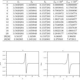
x0 = 40 with range [0,100] are taken. Error norms L2 and L∞ and conserved quanti-ties are illustrated in Table(3) for the time t = 20, together with results obtained with Ref.[28, 30]. It is seen that the predicted error norms L2 and L∞ are smaller than those obtained in Ref.[28, 30], and also invariants are reasonably in good agreement with their analytical values given by Eq.19. Percentage of relative changes ofI1,I2 and I3 are found 0.009×10−3 %,0.009×10−3 %,0.025×10−3 %,respectively. Moreover, the invariants

I1 and I2 change from their initial values by less than 3×10−7 and 1×10−7 respec-tively, during the time of running whereas, the change of invariant I3 approaches to zero throughout the run. Fig.(2) illustrates the motion of the solitary wave at diﬀerent time leves. Error distributions at timet= 10 and t= 20 are depicted graphically for solitary waves amplitudes 1 and 0.3 in Fig.(3). It is seen that the maximum errors are about the tip of the solitary waves and between−6×10−3 and 6×10−3, −2×10−4 and 2×10−4, respectively.

Table 1. Invariants and error norms for single solitary wave with c = 1,

h= 0.2, k= 0.025,0≤x≤100.

t I1 I2 I3 L2×103 _L ∞×103 0 4.4428660 3.2998251 1.4142022 0.00000000 0.00000000 1 4.4428662 3.2998252 1.4142023 1.01730104 0.54356142 2 4.4428667 3.2998257 1.4142028 2.02079556 1.08637566 3 4.4428671 3.2998261 1.4142031 3.00493932 1.59302250 4 4.4428674 3.2998264 1.4142033 3.97153841 2.08447826 5 4.4428676 3.2998265 1.4142034 4.92641719 2.57019590 6 4.4428677 3.2998266 1.4142035 5.87417096 3.05402949 7 4.4428678 3.2998266 1.4142035 6.81766748 3.53682732 8 4.4428678 3.2998266 1.4142035 7.75861590 4.01910803 9 4.4428678 3.2998266 1.4142035 8.69803722 4.50111164 10 4.4428678 3.2998266 1.4142035 9.23663428 4.98295436

0 20 40 60 80 100 -0.2

0.0 0.2 0.4 0.6 0.8 1.0

t=10 t=5 t=2 t=0

Figure 1. Single solitary wave with c = 1, h= 0.2,∆t = 0.025,0 ≤ x ≤ 100t= 0,2,5 and 10.

Table 2. Errors and invariants for single solitary wave with the order of convergence at c= 1, h= 0.2, k= 0.025,0≤x≤100, t= 10.

Method I1 I2 I3 L2×103 _L

∞×103

Analytical 4.44288 3.29983 1.41421 0 0

(8)

0 20 40 60 80 100 -0.2

0.0 0.2 0.4 0.6

t=20 t=10 t=5 t=0

Figure 2. Single solitary wave with c= 0.3, h= 0.1,∆t= 0.01,0≤x≤ 100 at level timest= 0,5,10 and 20.

Table 3. Invariants and error norms for single solitary wave withc= 0.3,

h= 0.1, k= 0.01,0≤x≤100.

t I1 I2 I3 L2×104 _L ∞×104 0 3.5820205 1.3450941 0.1537283 0.0000000 0.0000000 2 3.5820205 1.3450941 0.1537283 0.3959945 0.1793739 4 3.5820205 1.3450941 0.1537283 0.7903879 0.3500696 6 3.5820205 1.3450940 0.1537283 1.1833872 0.5158774 8 3.5820205 1.3450940 0.1537283 1.5741643 0.6800477 10 3.5820205 1.3450940 0.1537283 1.9627120 0.8456977 12 3.5820204 1.3450940 0.1537283 2.3494186 1.0096076 14 3.5820204 1.3450940 0.1537283 2.7346926 1.1724977 16 3.5820204 1.3450940 0.1537283 2.9188710 1.3347649 18 3.5820203 1.3450940 0.1537283 3.0022136 1.4966417 20 3.5820202 1.3450940 0.1537283 3.2849177 1.6582700 20[28] 3.58197 1.34508 0.153723 6.06885 2.96650 20[30] 3.582265 1.345182 0.1538901 3.379583 7.672911

0 20 40 60 80 100 -6.0x10

-3 -4.0x10 -3 -2.0x10 -3 0.0 2.0x10 -3 4.0x10 -3 6.0x10 -3

a)

E

r

o

r

x

0 20 40 60 80 100 -2.0x10

-4 -1.0x10 -4 0.0 1.0x10 -4 2.0x10 -4

b)

E

r

o

r

x

Figure 3. Error with a) c = 1, h= 0.2,∆t= 0.025, t = 10,0 ≤x ≤100 b) c= 0.3, h= 0.1,∆t= 0.01, t= 20,0≤x≤100.

5.2. Interaction of two solitary waves. For this problem, we study the behavior of the interaction of two solitary waves having diﬀerent amplitudes and travelling in the same direction. Initial condition of two well-seperated solitary waves of diﬀerent amplitudes has the following form:

U(x,0) = 2

∑

j=1

(9)

whereAj =√cj,pj =

√ _c

j

µ(cj+1),j= 1,2, cjandxj are arbitrary constants. The analytical

values of the conservation laws can be found from the Eq. (19) as

I1 = 2

∑

j=1

π√cj

pj

= 11.467698,

I2 = 2

∑

j=1

(

2cj

pj

+2µpjcj 3

)

= 14.629243, (21)

I3 = 2

∑

j=1

(

4c2_j

3pj − 2µpjcj

3

)

= 22.880466.

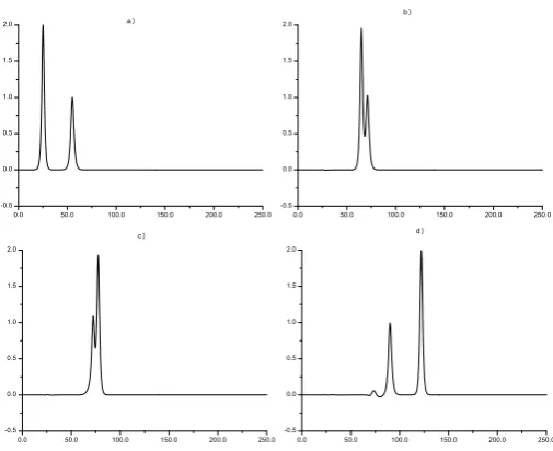
For the numerical simulation, we choose the parameters µ = 1, h = 0.2, k = 0.025, c1= 4, c2= 1, x1= 25, x2 = 55 over the interval 0≤x≤250 to coincide with those used by Ref.[28]. The calculations are performed from t = 0 to t = 20 and the values of the invariant quantitiesI1, I2 andI3 are recorded in Table(4). Table(4) displays a comparison of the values of the invariants obtained by the present method with those obtained in Ref. [28]. It is seen that the obtained values of the invariants remain almost constant during the computer run. Figure(4) illustrates the behaviour of the interaction of two solitary waves. It is observed from the Fig.(4) that at t= 0 the wave with larger amplitude is on the left of the second wave with smaller amplitude. Since the taller wave moves faster than the shorter one, it catches up and collides with the shorter one at t= 8 and then moves away from the shorter one as time increases. At t= 20, the amplitude of larger wave is 1.992788 at the point x = 127.2 whereas the amplitude of the smaller one is 0.994175 at the pointx= 92.2. It is found that the absolute diﬀerence in amplitude is 5.82×10−3 for the smaller wave and 7.2×10−3 for the larger wave for this algorithm.

Table 4. Comparison of invariants for the interaction of two solitary waves with results from [28] with h= 0.2, k= 0.025 in the region 0≤x≤250.

Present method [28]

t I1 I2 I3 I1 I2 I3 0 11.4677 14.6292 22.8803 11.4677 14.6291 22.8806 2 11.4675 14.6288 22.8785 11.4677 14.6292 22.8807 4 11.4673 14.6283 22.8766 11.4677 14.6292 22.8807 6 11.4672 14.6279 22.8747 11.4677 14.6295 22.8806 8 11.4684 14.6300 22.8793 11.4677 14.6451 22.8454 10 11.4682 14.6299 22.8784 11.4677 14.5963 22.8913 12 11.4663 14.6263 22.8704 11.4677 14.6287 22.8814 14 11.4664 14.6261 22.8687 11.4677 14.6295 22.8807 16 11.4664 14.6258 22.8669 11.4677 14.6294 22.8808 18 11.4663 14.6253 22.8650 11.4677 14.6293 22.8809 20 11.4661 14.6249 22.8631 11.4677 14.6292 22.8809

5.3. Interaction of three solitary waves. In this part, the behavior of the in-teraction of three solitary waves having diﬀerent amplitudes and travelling in the same direction are studied. We consider the MRLW equation with initial condition given by the linear sum of three well-seperated solitary waves of diﬀerent amplitudes

U(x,0) = 3

∑

j=1

(10)

0.0 50.0 100.0 150.0 200.0 250.0 -0.5

0.0 0.5 1.0 1.5 2.0

a )

0.0 50.0 100.0 150.0 200.0 250.0 -0.5

0.0 0.5 1.0 1.5 2.0

b )

0.0 50.0 100.0 150.0 200.0 250.0 -0.5

0.0 0.5 1.0 1.5 2.0

c )

0.0 50.0 100.0 150.0 200.0 250.0 -0.5

0.0 0.5 1.0 1.5 2.0

d )

Figure 4. Interaction of two solitary waves at a)t= 0, b)t= 8, c)t= 10,

d)t= 19.

where Aj = √cj, pj =

√ _c

j

µ(cj+1), j = 1,2,3, cj and xj are arbitrary constants. The

analytical values of the conservation laws can be found from the Eq.(19) as

I1 = 3

∑

j=1

π√cj

pj

= 14.9801,

I2 = 3

∑

j=1

(

2cj

pj

+ 2µpjcj 3

)

= 15.8218, (23)

I3 = 3

∑

j=1

(

4c2_j

3pj −

2µpjcj 3

)

= 22.9923.

To ensure an interaction of three solitary waves take place, calculation is carried out with the parameters µ = 1, h = 0.2, k = 0.025, c1 = 4, c2 = 1, c3 = 0.25, x1 = 15, x2 = 45, x3= 60 over the region 0≤x≤250.Simulations are run up to time t= 45.Table(5) compares the computed values of the invariants of the three solitary waves obtained by the Ref. [28]. It is observed that the obtained values of the invariants remain almost the same during the computer run and they are found to be very close to the values given in Ref. [28] which are all in good agreement with their analytical values given by Eq.(23). The absolute diﬀerence between the values of the conservative constants obtained by the present method at timest = 0 andt= 45 are ∆I1 = 2.67×10−2, ∆I2 = 8.5×10−3,∆I3 = 4.32×10−2. Figure(5) shows the interaction of these solitary waves at diﬀerent times. As it is seen from the Fig.(5),the interaction started about timet= 10,overlapping processes occured between timet = 15 and t = 40 and waves started to resume their original shapes after the timet= 40.

5.4. The Maxwellian initial condition. As our last problem, we have considered the evolution of an initial Maxwellian pulse into solitary waves using an initial condition of the form

(11)

Table 5. Comparison of invariants for the interaction of three solitary waves with results from [28] withh= 0.2, k = 0.025 in the region 0≤x≤

250.

Present method [28]

t I1 I2 I3 I1 I2 I3 0 14.9801 15.8375 23.0081 13.6891 15.4549 22.8816 5 14.9799 15.8365 23.0036 13.6891 15.3109 22.6939 10 14.9850 15.8453 23.0207 13.6891 15.6514 22.8388 15 14.9809 15.8367 22.9986 13.6891 15.6548 22.9347 20 14.9790 15.8340 22.9927 13.6891 15.6557 22.9330 25 14.9780 15.8323 22.9876 13.6892 156559 22.9336 30 14.9777 15.8311 22.9827 13.6894 15.6559 22.9348 35 14.9778 15.8299 22.9779 13.6913 15.6564 22.9343 40 14.9795 15.8291 22.9728 13.7015 15.6566 22.9335 45 14.9534 15.8290 22.9649 13.7043 15.6563 22.9303

0.0 50.0 100.0 150.0 200.0 250.0 -0.5

0.0 0.5 1.0 1.5 2.0

a )

0.0 50.0 100.0 150.0 200.0 250.0 -0.5

0.0 0.5 1.0 1.5 2.0

b )

0.0 50.0 100.0 150.0 200.0 250.0 -0.5

0.0 0.5 1.0 1.5 2.0

c )

0.0 50.0 100.0 150.0 200.0 250.0 -0.5

0.0 0.5 1.0 1.5 2.0

d )

Figure 5. Interaction of three solitary waves at a)t= 0, b)t= 5, c)t= 15,

d)t= 40.

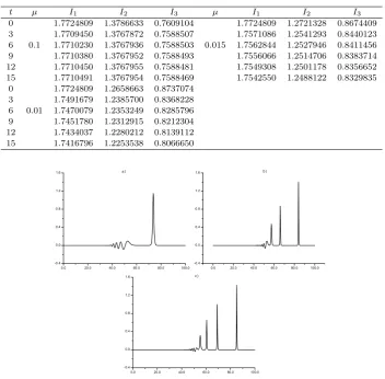
It is known that with the Maxwellian condition (24), the behavior of the solution de-pends on the values of µ. We study each of the following cases: µ = 0.1, µ = 0.015 and µ = 0.01. For µ = 0.1, only a single soliton is formed as shown in Fig.(5a). When

µ= 0.015,three stable solitons are formed as shown in Fig.(5b).Forµ= 0.01,four solitary waves are formed as shown in Fig. (5c). The peaks of the well developed wave lie on a straight line so that their velocities are linearly dependent on their amplitudes and also we observe a small oscillating tail appearing behind the last wave in all Maxwellian ﬁgures. The recorded values of the invariantsI1, I2 andI3 are given in Table(6).

6. Conclusion

(12)

Table 6. Invariants of MRLW equation using the Maxwellian initial condition.

t µ I1 I2 I3 µ I1 I2 I3 0 1.7724809 1.3786633 0.7609104 1.7724809 1.2721328 0.8674409 3 1.7709450 1.3767872 0.7588507 1.7571086 1.2541293 0.8440123 6 0.1 1.7710230 1.3767936 0.7588503 0.015 1.7562844 1.2527946 0.8411456 9 1.7710380 1.3767952 0.7588493 1.7556066 1.2514706 0.8383714 12 1.7710450 1.3767955 0.7588481 1.7549308 1.2501178 0.8356652 15 1.7710491 1.3767954 0.7588469 1.7542550 1.2488122 0.8329835

0 1.7724809 1.2658663 0.8737074 3 1.7491679 1.2385700 0.8368228 6 0.01 1.7470079 1.2353249 0.8285796 9 1.7451780 1.2312915 0.8212304 12 1.7434037 1.2280212 0.8139112 15 1.7416796 1.2253538 0.8066650

0.0 20.0 40.0 60.0 80.0 100.0 -0.4

0.0 0.4 0.8 1.2

1.6 a )

0.0 20.0 40.0 60.0 80.0 100.0 -0.4

0.0 0.4 0.8 1.2

1.6 b )

0.0 20.0 40.0 60.0 80.0 100.0 -0.4

0.0 0.4 0.8 1.2

1.6 c )

Figure 6. Maxwellian initial condition at t= 14.5 witha)µ= 0.1, b)µ= 0.015, c)µ= 0.01.

numerical solutions of the test problems, we have calculated the error norms L2 and

L_∞. The method successfully models the motion, the interaction of solitary waves and Maxwellian initial condition. The obtained results show that the Subdomain method using quartic B-spline shape functions is a remarkably successful numerical technique for solving the MRLW equation and can also be eﬃciently applied to a broad class of physically important non-linear partial diﬀerential equations.

References

[1] D. H. Peregrine, Calculations of the development of an undular bore, J. Fluid Mech. V.25,1966, pp.321-330.

[2] T. B. Benjamin, J. L. Bona and J. L. Mahoney, Model equations for long waves in nonlinear dispersive media,Phil. Trans. Roy. Soc. Lond. A 272, 1972, pp.47-78.

[3] J. L. Bona and P. J. Pryant, A mathematical model for long wave generated by wave makers in nonlinear dispersive systems,Proc. Cambridge Phil. Soc.V.73, 1973, pp.391-405.

[4] J. C. Eilbeck, G. R. McGuire, Numerical study of the regularized long wave equation, II:Interaction of solitary wave,J. Comput. Phys.V.19, N.1, 1975, pp. 43-57.

(13)

[6] D. Bhardwaj, R. Shankar, A computational method for regularized long wave equation, Comput. Math. Appl., V.40, N.12, 2000, pp. 1397-1404.

[7] Q. Chang, G. Wang, B. Guo, Conservative scheme for a model of nonlinear dispersive waves and its solitary waves induced by boundary motion, J. Comput. Phys.V.93, N.2, 1995, pp. 360-375. [8] L. R. T. Gardner, G. A. Gardner, Solitary waves of the regularized long wave equation, J. Comput.

Phys.V.91, 1990, pp.441-459.

[9] L. R. T. Gardner, G. A. Gardner, A. Dogan, A least-squares ﬁnite element scheme for the RLW equation,Commun. Numer. Meth. Eng.V.12, N.11, 1996, pp.795-804.

[10] L. R. T. Gardner, G. A. Gardner, I. Dag, A B-spline ﬁnite element method for the regularized long wave equation,Commun. Numer. Meth. Eng.V.11, N.1,1995, pp.59-68.

[11] M. E. Alexander, J. L. Morris, Galerkin method applied to some model equations for nonlinear dispersive waves,J. Comput. Phys.V.30, N.3, 1979, pp. 428-451.

[12] J. M. Sanz Serna, I. Christie, Petrov Galerkin methods for nonlinear dispersive wave, J. Comput. Phys. V.39 ,1981, pp.94-102.

[13] A.Dogan, Numerical solution of RLW equation using linear ﬁnite elements within Galerkin’s method, Appl. Math. Model., V.26, N.7, 2002, pp.771-783.

[14] A. Esen, S. Kutluay, Application of lumped Galerkin method to the regularized long wave equation, Appl. Math. Comput.V.174,N.2,2006, pp.833-845

[15] A. A. Soliman, K. R. Raslan, Collocation method using quadratic B-spline for the RLW equation, Int. J. Comput. Math.V.78, N.3, 2001, pp.399-412.

[16] A. A. Soliman, M. H. Hussien, Collocation solution for RLW equation with septic spline, Appl. Math. Comput.V.161, N.2, 2005, pp.623-636.

[17] K. R. Raslan, A computational method for the regularized long wave (RLW) equation,Appl. Math. Comput.V.167, N.2, 2005, pp.1101-1118.

[18] B. Saka, I. Dag and A. Dogan, Galerkin method for the numerical solution of the RLW equation using quadratic B-splines,Int. J. Comput. Math.V.81, N.6, 2004, pp.727-739.

[19] I. Dag, B. Saka, D. Irk, Application of cubic B-splines for numerical solution of the RLW equation, Appl. Math. Comput.V.159, N.2, 2004, pp.373-389.

[20] I. Dag, M. N. Ozer, Approximation of RLW equation by least-square cubic B-spline ﬁnite element method,Appl. Math. Model.V.25, N.3, 2001, pp.221-231.

[21] S. I .Zaki, Solitary waves of the splitted RLW equation,Comput. Phys. Commun. V.138, N.1, 2001, pp. 80-91.

[22] B. Y. Gou, W. M. Cao, The Fourier pseudo-spectral method with a restrain operator for the RLW equation, J. Comput. Phys.V.74, N.1, 1988, pp.110-126.

[23] L. Zhang, A ﬁnite diﬀerence scheme for generalized long wave equation, Appl. Math. Comput. V.168,N.2 2005,pp. 962-972.

[24] D. Kaya, S. M. El-Sayed, An application of the decomposition method for the generalized KdV and RLW equations, Chaos, Solitons and Fractals, V.17, N.5, 2003, pp.869-877.

[25] J. I. Ramos, Solitary wave interactions of the GRLW equation,Chaos, Solitons and Fractals, V.33, N.2, 2007, pp.479-491.

[26] T. Roshan, A Petrov-Galerkin method for solving the generalized regularized long wave (GRLW) equation, Comput. Math. Appl. V.63, N.5, 2012, pp.943-956.

[27] L. R. T. Gardner, G. A. Gardner, F. A. Ayoup, N. K. Amein, Simulations of solitary waves of the MRLW equation by B-spline ﬁnite element,Arab. J. Sci. Eng.V.22, 1997, pp. 183-193.

[28] A. K. Khalifa, K. R. Raslan, H. M. Alzubaidi, A collocation method with cubic B- splines for solving the MRLW equation, J. Comput. Appl. Math. V.212, N.2, 2008, pp.406-418.

[29] A. K. Khalifa, K. R. Raslan, H. M. Alzubaidi, A ﬁnite diﬀerence scheme for the MRLW and solitary wave interactions,Appl. Math. Comput.V.189, N.1, 2007, pp.346-354.

[30] K. R. Raslan, Numerical study of the modiﬁed regularized long wave equation, Chaos, Solitons and Fractals, V.42, N.3, 2009, pp.1845-1853.

[31] K. R. Raslan and S. M. Hassan, Solitary waves for the MRLW equation,Appl. Math. Lett.V.22, N.7, 2009, pp.984-989.

[32] S. B. Gazi Karakoc and T. Geyikli, Petrov-Galerkin ﬁnite element method for solving the MRLW equation,Mathematical Sciences, 7:25, 2013.

[33] F. Haq, S. Islam and I. A. Tirmizi, A numerical technique for solution of the MRLW equation usibng quartic B-splines,Appl. Math. Model.V.34, N.12, 2010, pp.4151-4160.

(14)

[35] P. M. Prenter,Splines and Variational Methods, (New York:John Wiley), (1975).

Seydi Battal Gazi Karakois now an assistant professor in Department of Mathematics at Nevsehir university ; Nevsehir (Turkey). He obtained his M.Sc. (2006) and Ph.D. (2011) degree from Inonu university. His re-search interests include numerical analysis, ﬁnite element methods, numeri-cal solutions of the partial diﬀerential equations, wave equations, variational methods. He has published articles journals related wave equations.

Turabi Geyikliis currently an assistant professor in Department of Math-ematics at Inonu university ; Malatya (Turkey). He got his Ph.D. (1994) degree from University of North Wales-U.K. His research interests include ﬁnite element methods, numerical solutions to partial diﬀerential equations, numerical analysis, wave equations, variational methods. He has published more than 10 articles.