DEMOGRAPHIC RESEARCH
A peer-reviewed, open-access journal of population sciences
DEMOGRAPHIC RESEARCH
VOLUME 38, ARTICLE 60, PAGES 1843–1884
PUBLISHED 8 JUNE 2018
http://www.demographic-research.org/Volumes/Vol38/60/ DOI: 10.4054/DemRes.2018.38.60
Research Article
Probabilistic projection of subnational total
fertility rates
Hana ˇSevˇc´ıkov´a
Adrian E. Raftery
Patrick Gerland
c
2018 ˇSevˇc´ıkov´a, Raftery & Gerland.
This open-access work is published under the terms of the Creative Commons Attribution 3.0 Germany (CC BY 3.0 DE), which permits use, reproduction, and distribution in any medium, provided the original author(s) and source are given credit.
1 Introduction 1844
2 Data 1846
3 Review of the national Bayesian hierarchical model 1850
4 Methods for subnational projections 1852
4.1 Scale method 1852
4.2 Scale-AR(1) 1853
4.3 One-directional BHM 1854
4.4 Correlation between regions 1855
5 Results 1856
5.1 TFR projections 1856
5.2 Out-of-sample predictive validation 1859
6 Discussion 1861
7 Acknowledgments 1863
References 1864
Probabilistic projection of subnational total fertility rates
Hana ˇSevˇc´ıkov´a1
Adrian E. Raftery2
Patrick Gerland3
Abstract
BACKGROUND
We consider the problem of probabilistic projection of the total fertility rate (TFR) for subnational regions.
OBJECTIVE
We seek a method that is consistent with the UN’s recently adopted Bayesian method for probabilistic TFR projections for all countries and works well for all countries.
METHODS
We assess various possible methods using subnational TFR data for 47 countries. RESULTS
We find that the method that performs best in terms of out-of-sample predictive perfor-mance and also in terms of reproducing the within-country correlation in TFR is a method that scales each national trajectory from the national predictive posterior distribution by a region-specific scale factor that is allowed to vary slowly over time.
CONCLUSIONS
Probabilistic projections of TFR for subnational units are best produced by scaling the national projection by a slowly time-varying region-specific scale factor. This supports the hypothesis of Watkins (1990, 1991) that within-country TFR converges over time in response to country-specific factors, and thus extends the Watkins hypothesis to the last 50 years and to a much wider range of countries around the world.
CONTRIBUTION
We have developed a new method for probabilistic projection of subnational TFR that
1Center for Statistics and the Social Sciences, University of Washington, Seattle, USA. Email:[email protected]. 2Departments of Statistics and Sociology, University of Washington, Seattle, USA.
works well and outperforms other methods. This also sheds light on the extent to which within-country TFR converges over time.
1. Introduction
The United Nations Population Division issued official probabilistic population projec-tions for all countries for the first time in 2015 (United Naprojec-tions 2015), using the method-ology described by Raftery et al. (2012). One of the key components of the projection methodology is a Bayesian hierarchical model for the total fertility rate (TFR) in all coun-tries (Alkema et al. 2011; Raftery, Alkema, and Gerland 2014; Fosdick and Raftery 2014). Population projections for subnational administrative units, such as provinces, states, counties, regions, or d´epartements (hereafter all referred to simply as regions), are of great interest to national and local governments for planning, policy, and decision-making (Rayer, Smith, and Tayman 2009). Typically these are used by policy and decision-makers at the national or subnational level.
A common current practice is to generate subnational projections deterministically by scaling national projections (US Census Bureau 2016). Specifically, the US Census Bureau provides a workbook for users to generate subnational TFR projections for up to 32 regions. The method requires the user to enter an ultimate TFR level (lower asymp-tote), to which the regional TFR converges, and a deterministic projection of the national TFR. The subnational TFR is then projected in such a way that it approaches the target TFR at the same rate as the national TFR approaches this target. The methods used by several other national agencies were reviewed by Rees et al. (2015), including methods used in Wales (Statistics for Wales 2017), Northern Ireland (NISRA 2014), and Canada (Statistics Canada 2014). These methods do not yield probabilistic projections.
We contrast two broad approaches to subnational probabilistic projection of TFR. One approach is a direct extension of the UN method (Alkema et al. 2011) to subnational data, effectively treating the country in the same way the UN model treats the world, and treating the regions in the same way the UN model treats the countries. Borges (2015) proposed an approach along these lines for the provinces of Brazil.
The other approach is motivated by the observation of Watkins (1990, 1991) that within-country variation in TFR in Europe decreased over the period of the fertility tran-sition there, between 1870 and 1960. This observation has been confirmed for a more re-cent period for the German-speaking countries (Basten, Huinink, and Kl¨usener 2012), to some extent for India (Arokiasmy and Goli 2012; Wilson et al. 2012), while the evidence is more equivocal for the United States (O’Connell 1981). Watkins posits that this was due to increased integration of national markets, expansion of the role of the state, and nation-building in the form of linguistic standardization over this period. Calhoun (1993) argues that, of these three mechanisms, only linguistic standardization clearly supports her argument.
However, some support for the importance of the role of the nation state for fertility is provided by the fact that nation states have specific and different policies aimed at affecting fertility rates (Tomlinson 1985; Chamie 1994), and some of these policies have been shown to be effective (Kalwij 2010; Luci-Greulich and Th´evenon 2013). Gauthier (2007) argues on the other hand that family policies have little impact. Note that Kl¨usener, Perelli-Harris, and Gassen (2013) investigated subnational convergence of non-marital fertility in Europe in recent decades and found that within-country variation increased. Similarly, de Beer and Deerenberg (2007) used a regression model to project differences in the level of fertility between Dutch municipalities and concluded that fertility is not likely to converge. These results are in contrast with the trends noted by other authors.
One question is then whether the direct extension of the UN method for countries to the subnational context adequately accounts for this tendency of TFR to converge within countries over time. Note that this extension of the UN method does predict within-country convergence of fertility rates over time during the fertility transition; the question is whether it adequately accounts for this convergence.
To investigate this question, we consider a different general approach, which starts from the national probabilistic projections produced by the UN method and then scales them for each region by a scaling factor that varies stochastically, but stays relatively constant. This induces more within-country correlation than the direct extension of the UN method. It could be viewed as a probabilistic extension of the method currently used by the US Census Bureau. It is also related to the method of Wilson (2013), but with some significant differences.
hypothesis of increasing within-country correlation, and they provide some guidance on how to carry out subnational probabilistic TFR projection.
Note that there is substantial literature on convergence of fertility rates in different countries to one another, with different conclusions argued (Wilson 2001, 2004; Reher 2004, 2007; Dorius 2008; Wilson 2011). Our work here has implications for within-country fertility convergence, but it is agnostic about fertility convergence between coun-tries and so does not have implications for global fertility convergence, for example.
The paper is organized as follows. We first describe the data used in this study and review the model for national probabilistic projections. We then introduce our proposed methodology for subnational probabilistic projections and present the results. The paper concludes with a discussion.
2. Data
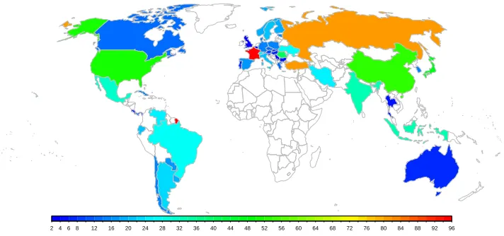
Figure 1: Map of 47 countries with subnational TFR data
2 4 6 8 12 16 20 24 28 32 36 40 44 48 52 56 60 64 68 72 76 80 84 88 92 96
Note: The color scale shows the number of regions for each country, which ranges from 2 to 96.
For statistical purposes, Eurostat has developed a Nomenclature of Territorial Units for Statistics for the European Union (NUTS, http://ec.europa.eu/eurostat/web/nuts/
overview). No equivalent statistical nomenclature exists at the international level for
other regions, but we provide a NUTS-equivalent assessment for regions outside Europe to assist the comparison between countries.
The subnational data used in this analysis has been compiled by the authors and are based on national data sources described in Table A-3 for each country. The reliability of this data varies between countries, but for a majority of the countries the fertility estimates are based on birth registration data. For Asian and Latin American countries which lack nationally representative vital registration, these fertility estimates are based on surveys and censuses. For all European countries for which Eurostat series are available, this data has been used, unless longer time series were available directly from national data sources.
The selection of countries used for this analysis is based on a combination of factors: (1) availability of fertility rates at subnational level for a meaningful length of time, (2) reasonably stable geographical divisions over time allowing meaningful comparisons, (3) sufficient population size to allow subnational disaggregation, (4) a range of countries covering different regions, to the extent possible, and (5) having completed most or all of the Phase II of their fertility transition at the national level.
representa-tive vital registration publishing fertility rates by subnational divisions. Several additional European countries could not be included in this analysis due to factors 1–3 that created substantial breaks in the time series due to major administrative changes or availability only for the most recent decade (e.g., Albania, Belarus, Bosnia and Herzegovina, Croatia, Ireland, Latvia, Luxembourg, Malta, Montenegro, Netherlands, TFYR Macedonia).
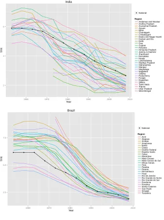
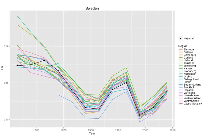
Figure 2 shows an example of the data for four countries (United States, India, Brazil, and Sweden). It illustrates that the data varies with respect to the correlation between regions. It also shows that the data started later than 1950 for some regions. In the figure, the national TFR from United Nations (2013) is shown as a black curve.
Figure 2: Observed data for regions of the United States, India, Brazil, and Sweden ● ● ● ● ● ● ● ● ● ● ● ● 2 3 4 5
1960 1970 1980 1990 2000 2010
Figure 2: (Continued) ● ● ● ● ● ● ● ● ● ● ● ● 2 4 6
1960 1970 1980 1990 2000 2010
Year
TFR
●National
Region
Andaman and Nicobar Andhra Pradesh Arunachal Pradesh Assam Bihar Chandigarh Chhattisgarh Dadra and Nagar Haveli Daman and Diu Delhi Goa Gujarat Haryana Himachal Pradesh Jammu & Kashmir Jharkhand Karnataka Kerala Lakshadweep Madhya Pradesh Maharashtra Manipur Meghalaya Nagaland Odisha Puducherry Punjab Rajasthan Sikkim Tamil Nadu Tripura Uttar Pradesh West Bengal India ● ● ● ● ● ● ● ● ● ● ● ● 2.5 5.0 7.5
1960 1970 1980 1990 2000 2010
Figure 2: (Continued)
● ●
●
●
●
● ●
● ●
● ●
●
1.5 2.0 2.5
1960 1970 1980 1990 2000 2010
Year
TFR
● National
Region Blekinge Dalarna Gavleborg Gotland Halland Jamtland Jonkoping Kalmar Kronoberg Norrbotten Orebro Ostergotland Skane Sodermanland Stockholm Uppsala Varmland Vasterbotten Vasternorrland Vastmanland Vastra Gotaland Sweden
Note: The national TFR is shown by the black curve.
3. Review of the national Bayesian hierarchical model
Our starting point for developing a methodology for subnational projections is the prob-abilistic model for projecting national TFR proposed by Alkema et al. (2011), which has now been adopted by the UN for its official projections. We start by summarizing the main ideas of this Bayesian hierarchical model (BHM). More detail can be found in Alkema et al. (2011) and Raftery, Alkema, and Gerland (2014).
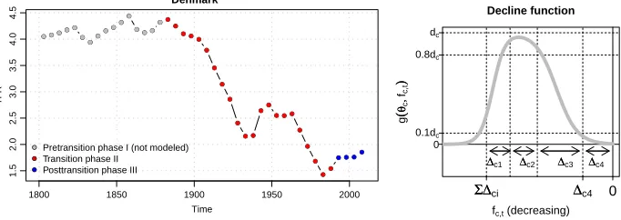
period (blue dots), during which fertility fluctuates at low levels, possibly recovering towards the replacement level.
Figure 3: Three phases of the typical TFR evolution for the example of Denmark (left); cartoon of a double logistic decline curve (right)
● ●●● ●● ●● ●●● ● ●● ● ● ●● ● ●● ● ● ● ● ● ● ● ●● ● ● ● ● ● ● ●● ● ● ●●
1800 1850 1900 1950 2000
1.5 2.0 2.5 3.0 3.5 4.0 4.5 Denmark Time TFR ● ● ● ●● ● ● ● ● ● ● ● ●● ● ● ● ● ● ● ●● ● ●●● ●● ●● ●●● ● ●● ● ● ● ● ●● ● ● ●
Pretransition phase I (not modeled) Transition phase II
Posttransition phase III
Decline function
fc,t (decreasing)
g
((
θθc
,,
fc,t
))
0
ΣΣ∆∆ci ∆∆c4 0
dc
0.8dc
0.1dc
∆∆c1 ∆∆c2 ∆∆c3 ∆∆c4
Note: The right panel shows a double logistic decline curve for countrycwith its parameters defining the shape.
fc,ton thexaxis denotes the TFR, whileg(θc,fc,t)on theyaxis denotes the first order difference in TFR.
To model the fertility declines in each five-year period during Phase II, a double logistic decline function is used. An example of this function is shown in the right panel of Figure 3. The function is parametrized by a set of country-specific parameters that define the shape of the country’s decline curve. Those parameters are drawn from a world distribution. The resulting BHM is estimated using Markov chain Monte Carlo (MCMC).
Phase III is modeled using a Bayesian hierarchical first-order autoregressive, or AR(1), process of the form:
fc,t+1−µc=ρc(fc,t−µc) +εc,t, with εc,t iid
∼N(0,σε2).
It implies that fertility for country c has a country-specific long-term mean, µc, and
autoregressive parameter, ρc, which are assumed to be drawn from a world
distribu-tion. The parameters of this world distribution in turn have a joint prior distribution, thus defining a three-level hierarchical model, where the three levels are the observation, the country, and the world. The resulting model is again estimated by MCMC.
parameters cannot be estimated. In such cases, the ‘world’ means and autoregressive pa-rameters are used. The estimated papa-rameters are then used to generate a set of future TFR trajectories yielding probabilistic TFR projections for all countries of the world.
4. Methods for subnational projections
Ideally, we seek a method for generating probabilistic subnational TFR projections that reflects the literature and theory of fertility transitions, is based on the national method-ology used by the UN and described above, works well for all countries, is as simple as possible, and yields correlations between regions that are similar to the correlations in the observed data.
We first describe a simple Scale method that provides an initial probabilistic exten-sion of methods used by the US Census Bureau and other national agencies. This simple approach works well from many points of view, but it does not allow for the possibility of crossovers between regions, whereas in fact these do happen. We therefore elaborate this model to allow the scale factor to change stochastically, but slowly over time, yielding the so-called Scale-AR(1) method. Finally we describe a quite different approach, called the one-directional BHM, which directly generalizes the national approach to the subnational context, allowing regions to vary more freely within a country.
4.1 Scale method
We start with a simple intuitive scale method where, for each trajectory from the prob-abilistic projection, the regional TFR is simply a product of the simulated national TFR and a time-independent but region-specific scale factor.
Letfc,t,idenote the national TFR projection for countrycat timetfrom trajectory
i, simulated from its posterior distribution as described above. We modelfrc,t,i, the TFR
for regionrcof countrycat timetin thei-th trajectory, by
frc,t,i=αrcfc,t,i, (1)
whereαrc denotes the regional scaling factor derived from the last observed (present)
time period denoted byP:
αrc=frc,t=P/fc,t=P. (2)
Note thatαrc is the same for all trajectories. This method yields a set of regional
Our numerical experiments, described below, indicated that this simple method per-formed surprisingly well. However, it also has a serious drawback. Scaling by a constant factor induces a perfect correlation, i.e., it does not allow for the possibility of crossovers between regions over time. However, such crossovers do happen, and the scale method says that they are impossible, which is not fully satisfactory.
4.2 Scale-AR(1)
To avoid this drawback, and modify the scale method so as to allow for the possibility of crossovers, we propose a variation of the simple Scale method where we model the regional scale factor using a first-order autoregressive, or AR(1), process:
αrc,t−1 =φ(αrc,t−1−1) +εrc,t, with εrc,t
iid
∼N(0,σ2c). (3)
The regional TFRfrc,t,i is then derived as in (1) with the additional lower bound
restriction,frc,t,i>0.5.
This model implies that the scaling factor will fluctuate around 1 in the long term. Regardless of its initial value, it will converge to a distribution that is centered around 1, and the rate of convergence is determined by theφparameter. We use the following settings for the model parameters, estimated from the data for all 47 countries available:
φ = 0.925, (4)
σ2c = min{σ2, (1−φ2)Varr∈Rc(αr,t=P)}, (5)
σ = 0.0452, (6)
where P again denotes the present time period and Rc denotes the set of regions of
countryc. The minimum restriction in (5) ensures that the variation ofα·,tacross regions
is not larger than the variation in the last observed time period, in line with the Watkins hypothesis and the long-term observed data.
We experimented with different methods of determining these parameters, including the use of country-specific values. The method we used is based on the asymptotic vari-ance ofαand yielded the best validation results. Reasonable changes inφandσmade very little difference to the results. Details of how these parameters were estimated are given in the appendix.
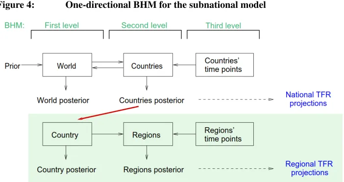
4.3 One-directional BHM
Next, we consider an extension of the world three-level BHM, which is depicted in Fig-ure 4. The three levels of this model are the world level, country level, and time point or observation level. In the world version, information from all countries is combined into the world level, which in turn influences the country level, yielding a two-directional BHM. The prior distribution of the hyperparameters is vague for most parameters, but also reflects expert knowledge in some cases. The model yields a posterior distribution of the world parameters, and the country-specific parameters, which is then used to generate the national projections.
Figure 4: One-directional BHM for the subnational model
Our extension has a similar setup, but moves down by one level of geography and works in one direction only. Thus the top level of our national model is the country, the next level is the region, and the bottom level is the time point. The upper level of our model corresponds to the country level of the world model; that is, we carry over the country-specific posterior from a world simulation and use it as the distribution of the hyperparameters in our national model (red arrow in Figure 4). On the lower level, data from all regions of a country is handled individually. The estimation of the regional parameters is informed by the hyperparameters, but the regional level does not influence the country level of the model. The resulting regional posterior distribution is used to project subnational TFR.
world posterior. As a result, all regions of those countries inherit the ‘world’ Phase III parameters.
4.4 Correlation between regions
For aggregating TFR over sets of regions, for example for deriving country’s averages, it is important to capture correlation in model errors between regions of a country, as was done by Fosdick and Raftery (2014) for capturing correlation between countries.
We will model the forecast errors as follows:
εt∼N(0, Σt=σt0Aσt), (7)
whereσt is a vector consisting of the forecast standard deviations for each region. For
Phase II this is the standard deviation of the errors in the double logistic model, and for Phase III it is the standard deviation of the error term in the AR(1) model. In (7),Ais a matrix where each elementAr,scorresponds to the correlation between the model errors
of country’s regionrandsover all time periods.
Letfr,t denote the observed TFR for region r at timet. We denote byer,t the
normalized forecast error, namely the forecast error divided by its standard deviation. The normalized forecast errorer,tis estimated as follows:
• Phase II: For each valuegr,t,iof a double logistic (DL) trajectoryiand the standard
deviation of DLσr,itakedr,t,i= (fr,t−gr,t,i)/σr,i. Thener,tis the mean ofdr,t,i
overi.
• Phase III: For each valuehr,t,iin a phase III trajectoryiand the standard deviation
of these trajectoriesσε,r,i, take the differencedr,t,i = (fr,t−hr,t,i)/σε,r,i. Then,
er,tis the mean ofdr,t,ioveri.
We define the correlation matrixAas
A=
¯
T −1
¯
T ˜
A+ 1
2 ¯T,
5. Results
We now compare results from the three methods described in the previous section. All three methods depend on a national BHM simulation. We used a simulation that was used to produce the official UN TFR projections in the WPP 2012 (United Nations 2013). Our version has 2,000 TFR trajectories for each country and was produced using the bayesTFR R package ( ˇSevˇc´ıkov´a, Alkema, and Raftery 2011).
For the Scale-AR(1) method, for each regionrc we set the initial scaling factor to
αrc,P = frc,P/fc,P withP being the last observed time period. Then we produced
projections ofαrc,tfor t > P using (3). Finally we applied (1), as in the case of the
simple Scale method, using each of the 2,000 TFR trajectories for countryc as fc,t,i.
This yielded 2,000 regional TFR trajectories.
For the one-directional BHM (1d-BHM), we ran the regional BHM while using the country posterior from the national BHM simulation. Then we projected 2,000 regional TFR trajectories using a sample of the regional posterior parameters. We explored two versions of this model, one that accounts for correlation between regions’ error terms and one that does not, the latter denoted by ‘1d-BHM (indep).’
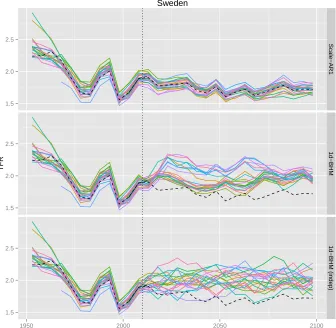
5.1 TFR projections
Figure 5: Observed data and one randomly selected projection trajectory for all regions of Sweden
1.5 2.0 2.5
1.5 2.0 2.5
1.5 2.0 2.5
Scale−AR1
1d−BHM
1d−BHM (indep)
1950 2000 2050 2100
TFR
Sweden
Note: The projections were obtained via three different methods: Scale-AR(1) (top), the one-directional BHM that accounts for correlation (center), and the one-directional BHM that treats regions independently (bottom). The vertical dotted line marks the last observed time period. The black dashed line marks the corresponding national trajectory.
if correlation is not taken into account, there are many more crossovers between regions than are typically seen in the past data.
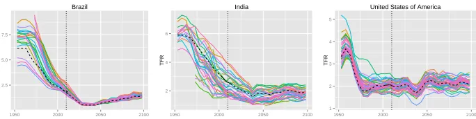
All the 47 countries in our dataset show the same pattern in terms of the differences between the methods. In Figure 6 we selected three countries for which one trajectory obtained via the Scale-AR(1) method is shown for each region (as in the top panel of Figure 5). As in the case of Sweden, the trajectories are highly correlated and closely follow the national trajectory.
Figure 6: Observed data and one randomly selected projection trajectory for each region, obtained via the Scale-AR(1) method for all regions of Brazil, India, and the United States
2.5 5.0 7.5
1950 2000 2050 2100
TFR
Brazil
2 4 6
1950 2000 2050 2100
TFR
India
1 2 3 4 5
1950 2000 2050 2100
TFR
United States of America
Note: The vertical dotted line marks the last observed time period. The black dashed line marks the corresponding national trajectory.
Showing one trajectory for each region, as in Figures 5 and 6, is a good way to see the correlation between regions. It must be the same trajectory, corresponding to the same set of parameters. A mean or median curve, which averages over trajectories, would not convey this information.
Figure 7: TFR projections for three regions of India
2 4 6
1950 2000 2050 2100
TFR
Assam
India
2 4 6
1950 2000 2050 2100
TFR
Uttar Pradesh
India
2 4 6
1950 2000 2050 2100
TFR
Goa
India
Note: Observed data and median projections are shown by the red line, and the 80% prediction interval is shown by the red shaded area. National data, projection median, and 80% prediction interval are shown as the gray line and the shaded area, respectively. The dotted line shows the median projection resulting from the simple Scale method.
Uttar Pradesh in the center is a type of region where current TFR is substantially higher than the national TFR. The underlying AR(1) process causes the median projection of such a region to converge to the national median in the long term, thus decreasing the gap between them. If simple scaling were applied, that gap would remain constant, resulting in much higher projections of TFR for the region.
Finally, Goa on the right, with its current TFR well below the national one, is pro-jected to increase on average, again yielding a smaller gap between the national and regional medians. Here simple scaling results in much lower projections.
Probabilistic projections for the regions of all 47 countries are provided in the sup-plementary material.
5.2 Out-of-sample predictive validation
We validated our methodology via predictive out-of-sample experiments, one for pre-dicting the period 1995–2010 and another one for prepre-dicting the period 1990–2010. We first assessed the various methods in terms of average predictive performance over all regions of the 47 countries. To assess their performance for predicting aggregates (and hence, for example, in capturing the between-region correlations), we further assessed the predictions of the average TFR across the regions of each country.
The results are shown in Table 1 for 1995–2010 and Table 2 for 1990–2010. The measures in the left part of each table (Marginal TFR) were derived by comparing the probabilistic projections of TFR for all regions to their observed values. The quantities in the right part of the tables (Average TFR) were derived by comparing a TFR averaged over all regions of each country with the observed average TFR for each country.
Table 1: Out-of-sample validation of probabilistic subnational TFR projections over 1995–2010
Marginal TFR Average TFR
MAE Bias CRPS 80% 95% MAE Bias CRPS 80% 95%
Scale-AR(1) 0.205 –0.088 –0.147 82.0 96.3 0.172 –0.117 –0.127 82.5 95.6 1d-BHM 0.228 –0.067 –0.167 75.1 90.1 0.169 –0.101 –0.123 71.5 89.1 1d-BHM (indep) 0.228 –0.071 –0.167 75.2 89.8 0.169 –0.103 –0.142 38.7 50.4 Scale 0.220 –0.106 –0.156 76.2 92.2 0.182 –0.136 –0.133 78.8 95.6
Persistence 0.365 –0.305 –0.365 – – 0.334 –0.303 –0.334 – –
Note: MAE is mean absolute error. CRPS is continuous ranked probability score, for which larger is better. The 80% and 95% columns refer to the percentage of the observations that fell within their prediction interval. The marginal TFR was validated on 3199 values; the average TFR was validated on 137 values. The Scale-AR(1) parameters wereφ= 0.898 andσ= 0.0533.
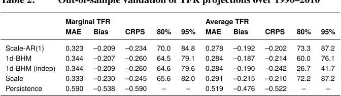
Table 2: Out-of-sample validation of TFR projections over 1990–2010
Marginal TFR Average TFR
MAE Bias CRPS 80% 95% MAE Bias CRPS 80% 95%
Scale-AR(1) 0.323 –0.209 –0.234 70.0 84.8 0.278 –0.192 –0.202 73.3 87.2 1d-BHM 0.344 –0.207 –0.260 64.5 79.1 0.284 –0.187 –0.214 60.0 76.1 1d-BHM (indep) 0.344 –0.209 –0.260 64.6 79.6 0.284 –0.190 –0.242 26.7 41.7 Scale 0.333 –0.230 –0.245 65.6 82.0 0.291 –0.215 –0.210 72.2 87.2
Persistence 0.590 –0.538 –0.590 – – 0.519 –0.476 –0.522 – –
Note: The marginal TFR was validated on 4144 values; the average TFR was validated on 180 values. The Scale-AR(1) parameters wereφ= 0.910 andσ= 0.0513.
For comparison purposes, we also added the Persistence method, in which the TFR stays at the same level over time, and so the forecast for all future time periods is equal to the last observed value. While this could be viewed as a straw man forecast, persistence forecasts have been found to perform surprisingly well in many forecasting contexts, and so it is worth making this comparison.
the coverage to be close to the nominal level. Thus, for example, ideally the coverage of the 80% interval would be close to 80%.
The appendix gives details of the derivation of these metrics. For MAE and bias, the smaller the absolute value the better. For the two coverage columns an ideal method would match the numbers to the corresponding percentage. The CRPS is a generalization of the MAE to the case of probabilistic forecast. It is a combination of an error-based and a variation-based measure that assesses the difference between the cumulative distribution function of the forecasts and the corresponding cumulative distribution function of the observations. Since it is an overall measure of the quality of the forecast, we give it a high weight when selecting the best method. In this case, a better method corresponds to a larger value of CRPS.
For the marginal TFR, the Scale-AR(1) method performed best in terms of CRPS, MAE, and coverage. The simple Scale method came in second. However, we would not recommend using the simple Scale method because it produces trajectories that are unrealistic in that they do not allow the possibility of crossovers between regions, as men-tioned previously. Note that by design, the Scale-AR(1) method yields larger uncertainty than the simple Scale method, which in this case translated to a better coverage and CRPS. The Scale method includes only the uncertainty from the national BHM model, whereas the Scale-AR(1) method has in addition the uncertainty included in the AR(1) process. There was essentially no difference between the 1d-BHM with and without correlation for the marginal TFR. This is expected, as the correlation plays a role only in aggregated indicators.
For the average TFR, the Scale-AR(1) and 1d-BHM had similar performance in terms of CRPS (one was better in Table 1, the other in Table 2). However, Scale-AR(1) had consistently better coverage. Here we see a big difference in coverage between the two versions of 1d-BHM, which does not have good performance if correlation between regions is not taken into account. The good performance of the Scale-AR(1) method suggests that it is accounting adequately for between-region spatial correlation.
6. Discussion
We have developed several methods for subnational probabilistic projection of TFR and applied them to data from 47 very diverse countries. All the methods take the national projections from the UN method as their starting point. We found that all the methods we propose performed well in terms of out-of-sample predictive performance and outper-formed a simple baseline persistence method.
this does not yield enough within-country correlation. Even when we introduce additional between-region correlation into this model, it still does not have enough within-country correlation overall.
We have compared several different methods, but there are still others in the lit-erature. Rayer, Smith, and Tayman (2009) considered ex-post assessment of predictive uncertainty for US counties, extending the national ex-post approach of Keyfitz (1981) and Stoto (1983) to the subnational context. Raymer, Abel, and Rogers (2012) used a vector autoregressive model for crude birth rates in three regions of England. While these methods may work well for developed countries that have had low fertility for an extended period, they do not capture the systematic variation in fertility decline rates among higher-fertility countries documented by Alkema et al. (2011), and so they may not be so appropriate for our goal here to develop a method applicable to countries at all levels of the fertility transition.
The extant method closest to our preferred Scale-AR(1) method is one proposed by Wilson (2013), who also proposed scaling a national TFR forecast by a region-specific scale factor that varies according to an AR(1) model and applied it to Sydney, Australia. However, there are several differences between the Scale-AR(1) method we propose here, and Wilson’s approach for TFR. The national TFR forecast used by Wilson is based on an AR(1) process centered around an externally specified main forecast. As discussed, this may not carry over well to higher-fertility countries. Our method, in contrast, is centered around the probabilistic forecast from the UN’s BHM, which is designed to work well for countries at all fertility levels and includes uncertainty about national projections. Also, in our method the model is statistically estimated, while in Wilson’s approach the parameters are adjusted manually.
Our preferred Scale-AR(1) method does not incorporate spatially-indexed between-region correlation. Instead, spatial correlation is modeled by a strong country effect. Our 1-d BHM method does incorporate spatial correlation in the variant that includes between-region correlation estimated from the data (especially methods 8–11 described in the Appendix section on estimating the error correlations). However, this did not allow us to include enough between-region correlation. This may be because within-country correlation seems to be dominated by a strong country effect rather than spatially indexed correlation, as can be seen for example for Sweden in Figure 5. This is also shown by the good calibration of the Scale-AR(1). Thus we feel it is likely that adding additional spatial correlation would not substantially improve fit of the model to the data at hand.
The Scale-AR(1) method is implemented as part of the R package bayesTFR ( ˇSevˇc´ıkov´a, Alkema, and Raftery 2011). The help page for the functiontfr.predict.subnat
gives details on how to use it. An R script to replicate results in this article is available on the journal’s website.
7. Acknowledgments
References
Abbasi-Shavazi, M. and McDonald, P. (2005). National and provincial-level fertility trends in Iran, 1972–2000. Canberra: Australian National University (Working Papers in Demography No. 94).
Alkema, L., Raftery, A.E., Gerland, P., Clark, S.J., Pelletier, F., Buettner, T., and Heilig, G.K. (2011). Probabilistic projections of the total fertility rate for all countries.
De-mography48(3): 815–839.doi:10.1007/s13524-011-0040-5.
Andreev, E. (2012). Age-specific fertility rates for Russia in 1959–2010 and regions in
1989–2010.
Andreev, E., Darsky, L., and Kharkova, T. (1998).Demographic history of Russia: 1927– 1959. Moscow: Informatika.
Arokiasmy, P. and Goli, S. (2012). Fertility convergence in the Indian states: An assess-ment of changes in averages and inequalities in fertility. Genus68: 65–88.
Australian Bureau of Statistics (2008). 3105.0.65.001: Australian Historial Pop-ulation Statistics, 2008. [electronic resource]. Canberra: Australian Bu-reau of Statistics. http://www.abs.gov.au/AUSSTATS/abs.nsf/Lookup/3105.0.65.
001Main+Features12008?OpenDocument.
Australian Bureau of Statistics (2010). 3101.0: Australian Demographic Statistics, June 2010. [electronic resource]. Canberra: Australian Bureau of Statistics.
Badan Pusat Statistik (2010). Fertilitas penduduk Indonesia: Hasil sensus penduduk 2010. Jakarta: Badan Pusat Statistik.
Basten, S., Huinink, J., and Kl¨usener, S. (2012). Spatial variation of sub-national fertility trends in Austria, Germany and Switzerland.Comparative Population Studies36(2–3): 12–52.doi:10.4232/10.CPoS-2011-08en.
Borges, G.M. (2015). Subnational fertility projections in Brazil: A Bayesian
probabilis-tic approach application. Poster presented at the Annual Meeting of the Population
Association of America, San Diego, USA, April 30–May 2, 2015.
Brenes, G. (2012). Evaluation of the 2011 census and demographic estimates for the period 1950–2011 [unpublished manuscript]. San Jose: Centro Centroamerican de Poblacion, Universidad de Costa Rica.
Calhoun, C. (1993). Book review:From provinces into nations: Demographic integration
in Western Europe, 1870–1960, by Susan Cotts Watkins. Journal of Modern History
65(3): 597–599. doi:10.1086/244688.
in 1990, 1995 and 1998–2011. Warsaw: Central Statistical Office of Poland.
Chamie, J. (1994). Trends, variations, and contradictions in national policies to in-fluence fertility. Population and Development Review 20(Supplement): 37–50.
doi:10.2307/2807938.
Czech Statistical Office (2012a). Demographic yearbooks 1982–1990. [electronic resource]. Prague: Czech Statistical Office. http://www.czso.cz/csu/redakce.nsf/i/
casova rada demografie.
Czech Statistical Office (2012b). Fertility in Czech Republic since 1991–2006: National
and regional level, NUTS3 and LAU1. Prague: Czech Statistical Office.
Czech Statistical Office (2012c). Demographic yearbook of the regions of the Czech Republic 2002–2011. [electronic resource]. Prague: Czech Statistical Office.
http://www.czso.cz/csu/2012edicniplan.nsf/engpubl/4027-12-engr2012.
de Beer, J. and Deerenberg, I. (2007). An explanatory model for projecting regional fertility differences in the Netherlands.Population Research and Policy Review26(5). Dorius, S.F. (2008). Global demographic convergence? A reconsideration of changing intercountry inequality in fertility. Population and Development Review34(3): 519–
537. doi:10.1111/j.1728-4457.2008.00235.x.
ECLAC and CELADE (2012a). Redatam+SP custom tabulations 10/26/2012 of Esti-maci´on Indirecta de la Fecundidad for Chile: Censo de Poblaci´on y Vivienda 1980– 2002 by regions. [electronic resource]. Santiago de Chile: Economic Commission for Latin America and the Caribbean and the Latin American and Caribbean Demographic Centre.http://www.redatam.org/redatam/en/.
ECLAC and CELADE (2012b). Redatam+SP custom tabulations 10/26/2012 of Esti-maci´on Indirecta de la Fecundidad for Brasil states: Censo de Poblaci´on y Vivienda 1980–2010 by states. [electronic resource]. Santiago de Chile: Economic Commission for Latin America and the Caribbean and the Latin American and Caribbean Demo-graphic Centre.http://www.redatam.org/redatam/en/.
ECLAC and CELADE (2012c). Redatam+SP custom tabulations 10/26/2012 of Esti-maci´on Indirecta de la Fecundidad for Ecuador: Censo de Poblaci´on y Vivienda 1982– 2010 by provinces. [electronic resource]. Santiago de Chile: Economic Commission for Latin America and the Caribbean and the Latin American and Caribbean Demo-graphic Centre.http://www.redatam.org/redatam/en/.
Cen-tre.http://www.redatam.org/redatam/en/.
ECLAC and CELADE (2012e). Redatam+SP custom tabulations 10/26/2012 of Esti-maci´on Indirecta de la Fecundidad for Panama: Censo de Poblaci´on y Vivienda 1990– 2010 by provinces. [electronic resource]. Santiago de Chile: Economic Commission for Latin America and the Caribbean and the Latin American and Caribbean Demo-graphic Centre.http://www.redatam.org/redatam/en/.
ECLAC and CELADE (2012f). Redatam+SP custom tabulations 10/26/2012 of Esti-maci´on Indirecta de la Fecundidad for Paraguay: Censo de Poblaci´on y Vivienda 1982–2002 by departments. [electronic resource]. Santiago de Chile: Economic Com-mission for Latin America and the Caribbean and the Latin American and Caribbean Demographic Centre.http://www.redatam.org/redatam/en/.
ECLAC and CELADE (2012g). Redatam+SP custom tabulations 10/26/2012 of Es-timaci´on Indirecta de la Fecundidad for Uruguay: Censo de Poblaci´on y Vivienda 1985–2011 by departments. [electronic resource]. Santiago de Chile: Economic Com-mission for Latin America and the Caribbean and the Latin American and Caribbean Demographic Centre.http://www.redatam.org/redatam/en/.
ECLAC and CELADE (2012h). Redatam+SP custom tabulations 10/26/2012 of Esti-maci´on Indirecta de la Fecundidad for Venezuela: Censo de Poblaci´on y Vivienda 1990–2011 by states. [electronic resource]. Santiago de Chile: Economic Commission for Latin America and the Caribbean and the Latin American and Caribbean Demo-graphic Centre.http://www.redatam.org/redatam/en/.
ESCAP (1987). Levels and trends of fertility in Indonesia based on the 1971 and 1980
population censuses: A study of regional differentials. Bangkok: United Nations,
Eco-nomic and Social Commission for Asia and the Pacific.
Eurostat (2012). Fertility rates by age and NUTS 2 region. [electronic resource]. Lux-embourg: Eurostat. http://ec.europa.eu/eurostat/web/products-datasets/product?code=
demo r frate2.
Fosdick, B.K. and Raftery, A.E. (2014). Regional probabilistic fertility forecasting by modeling between-country correlations. Demographic Research30(35): 1011–1034.
doi:10.4054/DemRes.2014.30.35.
Gauthier, A.H. (2007). The impact of family policies on fertility in industrialized coun-tries: A review of the literature. Population Research and Policy Review26(3): 323–
346.doi:10.1007/s11113-007-9033-x.
Germany Federal Statistical Office (2012).Zusammengefasste Geburtenziffer (total fertil-ity rate) auf Bundeslandebene (Einheit: Kinder je Frau) for 1990–2010 by Bundesland:
Gneiting, T. and Raftery, A.E. (2007). Strictly proper scoring rules, prediction, and estimation. Journal of the American Statistical Association 102(477): 359–378.
doi:10.1198/016214506000001437.
Gullickson, A. (2001). Multiregional probabilistic forecasting [unpublished manuscript]. Berkeley: University of California. http://u.demog.berkeley.edu/aarong/PAPERS/
gullick iiasa stochmig.pdf.
Gullickson, A. and Moen, J. (2001). The use of stochastic methods in local area population forecasts [unpublished manuscript]. Berkeley: University of Cal-ifornia. http://www.demog.berkeley.edu/aarong/PAPERS/gullickmoen paa2001
stochminn.pdf.
Hersbach, H. (2000). Decomposition of the continuous ranked probability score for en-semble prediction systems.Weather and Forecasting15: 559–570.
doi:10.1175/1520-0434(2000)015¡0559:DOTCRP¿2.0.CO;2.
Hirschman, C. (1994). Why fertility changes. Annual Review of Sociology20(1): 203–
233. doi:10.1146/annurev.soc.20.1.203.
IBGE (2012). Tfr estimates by Brazilian states for 1940–2000 from census data and for 2001–2009 from Pesquisa Nacional por Amostra de Domic´ılios (PNAD) survey data (TFR BY Brazil 1940-2009.xlsx). [electronic resource]. Rio de Janeiro: Instituto Brasileiro de Geografia e Estat´ıstica.https://www.ibge.gov.br/english/.
INDEC (2012). Din´amica y estructura de la poblaci´on: Tasa bruta de natalidad por provincia: A˜nos 1980–2009. [electronic resource]. Canberra: Instituto Nacional de Estad´ıstica y Censo. https://web.archive.org/web/20131114005930/http://www.indec.
gov.ar/principal.asp?id tema=7924.
INE (2012). Demograf´ıa y poblaci´on. [electronic resource]. Madrid: Instituto Nacional de Estad´ıstica. http://www.ine.es/dyngs/INEbase/es/categoria.htm?c=Estadistica
Pcid=1254734710990.
INE Chile (2012). TFR estimates for 1997–2010 by Chilean regions. [elec-tronic resource]. Santiago de Chile: Instituto Nacional de Estad´ısticas.
http://palma.ine.cl/demografia/SELECCION INDICADORES.aspx.
INSEE (2006). Donn´ees de d´emographie r´egionale 1954 `a 1999: CD-ROM. Paris: Institut National de la Statistique et des ´Etudes ´Economiques.
INSEE (2012). 1990–2009 statistiques de l’´etat civil et estimations de population: Tableau p3d: Indicateurs g´en´eraux de population par d´epartement et r´egion. [elec-tronic resource]. Paris: Institut National de la Statistique et des ´Etudes ´Economiques.
ISTAT (2012). Serie storiche: Tavola 2.7.1. [electronic resource]. Rome: Italian National Institute of Statistics.http://seriestoriche.istat.it/index.php?id=1no cache=1L=1. Kalwij, A. (2010). The impact of family policy expenditure on fertility in Western
Eu-rope. Demography47(2): 503–519. doi:10.1353/dem.0.0104.
Keyfitz, N. (1981). The limits of population forecasting. Population and Development
Review7(4): 579–593.doi:10.2307/1972799.
Kl¨usener, S. (2012). TFR by Laender for selected years covering 1950–2008: Courtesy
of Frank Swiaczny. Rostock: Max Planck Institute for Demographic Research.
Kl¨usener, S., Perelli-Harris, B., and Gassen, N.S. (2013). Spatial aspects of the rise of nonmarital fertility across Europe since 1960: The role of states and regions in shaping patterns of change. European Journal of Population 29(2): 137–165.
doi:10.1007/s10680-012-9278-x.
Lee, R., Miller, T., and Edwards, R.D. (2003). The growth and aging of California’s pop-ulation: Demographic and fiscal projections, characteristics and service needs. Berke-ley: University of California (CEDA Papers, Special Report).
Lincot, L. and Lutinier, B. (2006). Les evolutions demographiques departementales et
regionales entre 1975 et 1994. Paris: Institut National de la Statistique et des ´Etudes
´
Economiques.
Linder, F. and Grover, R. (1947). Vital statistics rates in the United States 1900–1940. Washington, D.C.: National Office of Vital Statistics.
Luci-Greulich, A. and Th´evenon, O. (2013). The impact of family policies on fertil-ity trends in developed countries. European Journal of Population29(4): 387–416.
doi:10.1007/s10680-013-9295-4.
National Bureau of Statistics of China (1993). Data of the 1990 Population Census of
China. Beijing: China Statistical Publishing House.
National Bureau of Statistics of China (2002).Tabulation on the 2000 Population Census
of China. Beijing: China Statistical Publishing House.
National Bureau of Statistics of China (2007).Results of the 2005 national 1% population
sample census. Beijing: China Statistical Publishing House.
National Bureau of Statistics of China (2012).Tabulation on the 2010 Population Census
of the People’s Republic of China. Beijing: China Statistical Publishing House.
National Bureau of Statistics of China and East-West Centre (2007). Fertility estimates
for provinces of China: 1975–2000. Beijing: China Statistical Publishing House.
Demo-graphic sourcebook: Vital statistics for 1930–2003 by prefectures. [electronic re-source]. Tokyo: Ministry of Health, Labour and Welfare. http://www8.cao.go.jp/
shoushi/whitepaper/w-2004/html-h/html/g3400000.html.
National Institute of Statistics of Romania (2006). Demographic yearbook 2006: Table
7: Live births and live-birth rate by counties, 1966–2005. Bucharest: National Institute
of Statistics.
National Institute of Statistics of Romania (2012). Evenimente demografice ˆın anul 1993– 2010: Indicatorul conjunctural al fertilitatii by counties: Table 23 for 1993, table 22 for 1994, tables 34 for 1995–2010). [electronic resource]. Bucharest: National Institute of Statistics.http://www.insse.ro.
National Statistical Institute of Bulgaria (no year). Population: Demography, mi-gration and projections). [electronic resource]. Sofia: National Statistical In-stitute. http://www.nsi.bg/en/content/6593/population-demography-migration-and-projections.
National Statistics Office of Thailand (1997). Report on the 1995–1996 Survey of
popu-lation change. Bangkok: National Statistics Office.
NCHS (1977). Birth and fertility rates for states and metropolitan areas. Hyattsville: National Center for Health Statistics (DHEW Publication No. (HRA) 78-1905). NCHS (no year). Vital statistics data. [electronic resource]. Hyattsville: National Center
for Health Statistics. https://www.cdc.gov/nchs/data access/vitalstatsonline.htm. NISRA (2014). Population projections for areas within Northern Ireland:
2014-based. Belfast: Northern Ireland Statistics and Research Agency (Methodol-ogy Paper).
https://www.nisra.gov.uk/sites/nisra.gov.uk/files/publications/SNPP14-Methodology.pdf.
O’Connell, M. (1981). Regional fertility patterns in the United States: Con-vergence or diCon-vergence? International Regional Science Review 6(1): 1–14.
doi:10.1177/016001768100600101.
Office F´ed´eral de la Statistique (2012). Indicateur conjoncturel de f´econdit´e selon le
canton. Neuchˆatel: Office f´ed´eral de la statistique. https://www.bfs.admin.ch/bfs/de/
home/statistiken/bevoelkerung.assetdetail.3442623.html.
Office of the Registrar General and Census Commissioner (no year). 1971–2010 sam-ple registration system. [electronic resource]. New Delhi: Office of the Registrar General and Census Commissioner. http://www.censusindia.gov.in/2011-Common/
Sample Registration System.html.
Tomo I. Havana: Oficina Nacional de Estad´ısticas de Cuba.
Oficina Nacional de Estad´ısticas de Cuba (2005b). anuario demogr´afico de Cuba 2005– 2011. [electronic resource]. Havana: Oficina Nacional de Estad´ısticas de Cuba.
http://www.one.cu/PublicacionesDigitales/PublicacionesDigitales.asp?cod=A.
ONS (2012). Total fertility rates for the UK and its constituent countries for 1938–2010. [electronic resource]. London: Office for National Statistics, Vital Statistics Outputs Branch.http://www.ons.gov.uk/ons/datasets-and-tables/index.html.
Pantelides, E.A. (1989).La fecundidad adolescente en la Argentina al comienzo del Siglo XXI. Buenos Aires: Centro de Estudios de Poblaci´on.
Pantelides, E.A. (2006). La transicion de la fecundidad en la Argentina 1869–1947. Buenos Aires: Centro de Estudios de Poblaci´on.
Partida Bush, V. (2008). Proyecciones de la poblaci´on de m´exico, de las entidades fed-erativas, de los municipios y de las localidades 2005–2050. Mexico City: Consejo Nacional de Poblaci´on (Documento metodol´ogico).
PCO and DPS (1985).1982 Population Census of China: Results of computer tabulation. Beijing: China Statistical Publishing House.
Pejaranonda, C. (1985). Declines in fertility by district in Thailand: An analysis of the
1980 census. Bangkok: United Nations, Economic and Social Commission for Asia
and the Pacific.
Raftery, A.E., Alkema, L., and Gerland, P. (2014). Bayesian population projections for the United Nations.Statistical Science29(1): 58–68.doi:10.1214/13-STS419. Raftery, A.E., Li, N., ˇSevˇc´ıkov´a, H., Gerland, P., and Heilig, G.K. (2012). Bayesian
prob-abilistic population projections for all countries.Proceedings of the National Academy
of Sciences109(35): 13915–13921. doi:10.1073/pnas.1211452109.
Ram, U. and Ram, F. (2009). Fertility in India: Policy issues and program challenges. In: Singh, K., Yadava, R., and Pandey, A. (eds.).Population, poverty and health:
Analyti-cal approaches. New Delhi: Hindustan: 45–67.
Rayer, S., Smith, S.K., and Tayman, J. (2009). Empirical prediction intervals for county population forecasts. Population Research and Policy Review28: 773–793.
doi:10.1007/s11113-009-9128-7.
Raymer, J., Abel, G.J., and Rogers, A. (2012). Does specification matter? Experiments with simple multiregional probabilistic population projections.Environment and
Plan-ning A44(11): 2664–2686.doi:10.1068/a4533.
popula-tion forecasting. Paper presented at the GeoComputation 98 conference, Bristol, UK, September 17–19, 1998.
Rees, P., Wohland, P., Norman, P., and Lomax, N. (2015). Sub-national projection meth-ods for Scotland and Scottish areas: A review and recommendations. Leeds: White Rose University Consortium, University of Leeds (Research report).
Reher, D.S. (2004). The demographic transition revisited as a global process.Population,
Space and Place10(1): 19–41. doi:10.1002/psp.313.
Reher, D.S. (2007). Towards long-term population decline: A discussion of relevant numbers. European Journal of Population23(2): 189–207. doi:10.1007/s10680-007-9120-z.
Rele, J. (1987). Fertility levels and trends in India, 1951–1981. Population and
Develop-ment Review13(3): 513–530. doi:10.2307/1973137.
Rele, J. (1988). 70 years of fertility change in Korea: New estimates from 1916 to 1985.
Asia-Pacific Population Journal3(2): 29–54.
Rosero-Bixby, L. (2012). Estimates of fertility in the provinces of Costa Rica 1956–2011 [unpublished manuscript]. San Jose: Centro Centroamerican de Poblacion, Universi-dad de Costa Rica.
Russian Federal State Statistics Service (2012). Age-specific fertility rates per regions
for 1978–1979, 1982–1983, 1984–1985, 1986–1987, 1988–1989. Moscow: Russian
Federal State Statistics Service.
ˇSevˇc´ıkov´a, H., Alkema, L., and Raftery, A.E. (2011). bayesTFR: An R package for probabilistic projections of the total fertility rate.Journal of Statistical Software43(1): 1–29.doi:10.18637/jss.v043.i01.
Shorter, F., Macura, M., and the Panel on Turkey (1982).Trends in fertility and mortality
in Turkey, 1935–1975. Washington, D.C.: National Academy Press.
Smith, S.K. and Sincich, T. (1988). Stability over time in the distribution of population forecast errors.Demography25(3): 461–474.
Smith, S.K. and Tayman, J. (2004).Confidence intervals for population forecasts: A case
study of time series models for states. Paper presented at the Population Association of
America Meeting, Boston, USA, April 1–3, 2004.
State Statistics Service of Ukraine (2012). Population. [electronic resource]. Kiev: State Statistics Service of Ukraine. http://database.ukrcensus.gov.ua/MULT/
Database/Population/databasetree en.aspandhttp://www.ukrstat.gov.ua/druk/katalog/
Statistical Centre of Iran (2001). Estimation of levels and patterns of fertility in Iran:
With application of own-children method (1972–1996). Tehran: Statistical Centre of
Iran.
Statistical Office of the Republic of Serbia (2012). Demographic yearbook 2002 and
2003: Table 2-11: General, specific and total fertility rates, 1950–2003, by regions.
Belgrade: Statistical Office of the Republic of Serbia, Division of Demography. Statistical Office of the Republic of Slovenia (2012). Basic data on total
fer-tility rates, statistical regions, Slovenia, annually for 2002 onward. [elec-tronic resource]. Ljubljana: Statistical Office of the Republic of
Slove-nia. http://pxweb.stat.si/pxweb/Dialog/varval.asp?ma=05J2008Eti=path=../Database/
Demographics/05 population/30 Fertility/10 05J20 Fertility RE OBC/lang=1.
Statistical Office of the Slovak Republic (2012). Age-specific live births, female popula-tion, and fertility rates for 1996–2010 by regions (NUTS 3) and the Slovak Republic
(K´opia - up hmr cmr 1996-2010 kraje sj.xls). Bratislava: Statistical Office of the
Slo-vak Republic.
Statistics Austria (2012). Geborene: Langfristiger Trend. [electronic resource]. Vienna: Statistics Austria. http://statistik.at/web de/statistiken/menschen und gesellschaft/
bevoelkerung/geborene/index.html.
Statistics Belgium (2012). Tableaux sur les naissances et f´econdit´e: Table 24: Taux de f´econdit´e selon l’ˆage des femmes atteint dans l’ann´ee, de 15 `a 49 ans pour le pays et les regions (NI 03.24 historique FR v4.xls). [electronic resource]. Brussels: Statis-tics Belgium, Direction g´en´erale Statistique et Information ´economique: Direction th´ematique Soci´et´e.http://statbel.fgov.be/fr.
Statistics Canada (2012). Births and total fertility rate, by province and territory. [elec-tronic resource]. Ottawa: Statistics Canada.https://www.statcan.gc.ca/tables-tableaux/
sum-som/l01/cst01/hlth85b-eng.htm.
Statistics Canada (2014). Population projections for Canada (2013 to 2063), provinces and territories (2013 to 2038): Technical report on methodology and assumptions. Ottawa: Statistics Canada (Statistics Canada Catalogue 91-620-X).
http://www.statcan.gc.ca/pub/91-620-x/91-620-x2014001-eng.htm.
Statistics Denmark (2012). StatBank. [electronic resource]. Copenhagen: Statistics Denmark. http://www.statbank.dk/statbank5a/default.asp?w=1280.
Statistics Finland (2012). Total fertility rate by region 1987–2011. [electronic resource]. Helsinki: Statistics Finland.http://tilastokeskus.fi/index en.html.
Statistics for Wales (2017). Sub-national projections for Wales. Cardiff: Welsh Govern-ment (Technical report).
http://gov.wales/docs/statistics/2017/171019-local-authority-population-projections-technical-en.pdf.
Statistics Korea (2012). KOSIS 1970–2011 statistics table for live births, crude birth rate and total fertility rate by province. [electronic resource]. Seoul: Statistics Korea.
http://kosis.kr/statHtml/statHtml.do?orgId=101tblId=DT 1B81A21.
Statistics Norway (2012). StatBank Table 08556: Total fertility rate and age-specific fertility rates for 5-year periods. [electronic resource]. Oslo: Statistics Norway.
http://www.ssb.no/en/table/08556.
Statistics of Japan (2012). 2010 vital statistics of Japan: Volume 1: Natality, table 4.5: Trends in total fertility rates by each prefecture for 1960–2010. [electronic resource]. Tokyo: Ministry of Health, Labour and Welfare. http://www.e-stat.go.jp/SG1/estat/
CsvdlE.do?sinfid=000012659212.
Statistics Portugal (2012). Demographic indicators: Total fertility rate (no.) by place of residence (NUTS – 2002). [electronic resource]. Lisboa: Statistics Portugal. https://ine.pt/xportal/xmain?xpid=INExpgid=ine indicadoresindOcorrCod=
0000600contexto=ptiselTab=tab10.
Statistics Sweden (1999). Befolkningsutvecklingen under 250 ˚ar: Historisk statistik f¨or
Sverige [Population development in Sweden in a 250-year perspective]. Stockholm:
Statistiska centralbyr˚an.
Statistics Sweden (2012a). Population by region, marital status, age and sex for 1968–2011. [electronic resource]. Stockholm: Statistiska centralbyr˚an.
http://www.statistikdatabasen.scb.se/pxweb/en/ssd/START BE BE0101 BE0101A/
BefolkningNy/?rxid=86abd797-7854-4564-9150-c9b06ae3ab07.
Statistics Sweden (2012b). Live births by region, mothers age and childs sex for 1968–2011. [electronic resource]. Stockholm: Statistiska centralbyr˚an.
http://www.statistikdatabasen.scb.se/pxweb/en/ssd/START BE BE0101 BE0101H/
FoddaK/?rxid=86abd797-7854-4564-9150-c9b06ae3ab07.
Stoto, M.A. (1983). The accuracy of population projections. Journal of the American
Statistical Association78(381): 13–20. doi:10.1080/01621459.1983.10477916.
Tayman, J. (2011). Assessing uncertainty in small area forecasts: State of the practice and implementation strategy. Population Research and Policy Review30(5): 781–800.
Tayman, J., Schafer, E., and Carter, L. (1998). The role of population size in the deter-mination and prediction of population forecast errors: An evaluation using confidence intervals for subcounty areas. Population Research and Policy Review17(1): 1–20.
doi:10.1023/A:1005766424443.
Tomlinson, R. (1985). The ‘disappearance’ of France, 1896–1940: French politics and the birth rate.Historical Journal28(2): 405–415.doi:10.1017/S0018246X00003198. UNFPA (2011). Impact of demographic change in Thailand. Bangkok: United Nations
Population Fund.
United Nations (2013). World population prospects: The 2012 revision. New York: United Nations.
United Nations (2015). World population prospects: The 2015 revision, probabilistic
population projections. New York: Population Division, Department of Economic and
Social Affairs, United Nations.
United Nations (2017). World population prospects: The 2017 revision. New York: Population Division, Department of Economic and Social Affairs, United Nations.
http://esa.un.org/unpd/wpp.
US Census Bureau (2016). Subnational projections toolkit: Methods: Projtfr32. [elec-tronic resource]. Suitland: US Census Bureau. https://www2.census.gov/software/
sptoolkit/documentation/projtfr32-methods.pdf.
US Census Office (1902). 1900 census: Volume III: Vital statistics, Part 1: Analy-sis and ratio tables. [electronic resource]. Washington, D.C.: US Census Office.
https://www.census.gov/library/publications/1902/dec/vol-03-vital-stats.html.
Wanner, P. (2000). Caract´eristiques des r´egimes d´emographiques des cantons suisses 1870–1996. In: Association Internationale des D´emographes de Langue Franc¸aise (ed.).Colloque international de la Rochelle, 22–26 septembre 1998. Paris: Presses Universitaires de France: 243–253.
Watkins, S.C. (1990). From local to national communities: The transformation of demo-graphic regimes in Western Europe, 1870–1960.Population and Development Review
16(2): 241–272. doi:10.2307/1971590.
Watkins, S.C. (1991).From provinces into nations: Demographic integration in Western
Europe, 1870–1960. Princeton: Princeton University Press.
Wilson, C. (2001). On the scale of global demographic convergence 1950– 2000. Population and Development Review 27(1): 155–171.
doi:10.1111/j.1728-4457.2001.00155.x.
doi:10.1126/science.304.5668.207c.
Wilson, C. (2011). Understanding global demographic convergence since 1950.
Population and Development Review 37(2): 375–388.
doi:10.1111/j.1728-4457.2011.00415.x.
Wilson, C., Singh, A., Singh, A., and Pallikadavath, S. (2012). Convergence and
con-tinuity in Indian fertility: A long-run perspective, 1871–2008. Paper presented at the
Annual Meeting of the Population Association of America, San Francisco, US, May 3–5, 2012.http://paa2012.princeton.edu/abstracts/120470.
Wilson, T. (2013). Quantifying the uncertainty of regional demographic forecasts.
Ap-plied Geography42: 108–115.doi:10.1016/j.apgeog.2013.05.006.
Wilson, T. and Bell, M. (2007). Probabilistic regional population forecasts: The example of Queensland, Australia. Geographical Analysis 29(1): 1–25.
doi:10.1111/j.1538-4632.2006.00693.x.
Appendix: Methods
Estimation of the Scale-AR(1) parameters
Here we give details on estimating parameters of the Scale-AR(1) model.
The model is based on an AR(1) process for region-specific scale factorsαrc,tcentered
at one, namely
αrc,t−1 =φ(αrc,t−1−1) +εrc,t, with εrc,t
iid
∼N(0,σc2). (8)
We impose the restriction that the scale factors not diverge indefinitely over time. We implement this by requiring thatσ2
c is such that
lim
t→∞Var(αrc,t)≤Varq∈Rc(αq,t=P), (9)
wherePdenotes the present time period andRcdenotes the set of regions in country
c. This yields
σc2= min{σ2, (1−φ2)Varr∈Rc(αr,t=P)}. (10)
We are interested in estimating the country- and region-independent parametersφand
σ. We know from the observed data that the standard deviation ofαrc,tdeclines as
TFR declines, which is also in line with the theoretical expectations of Watkins (1990, 1991). Thus we need to find asymptotic values for those parameters.
Let∆αrc,tdenote the first order differences over time, namely
∆αrc,t=αrc,t−αrc,t−1. (11)
Then
lim
t→∞Var(αrc,t) =
σ2
1−φ2 and (12)
lim
t→∞Var(∆αrc,t) = 2(1−φ)Var(αrc,t). (13)
Equations (12) and (13) imply that
φ = 1−Var(∆αrc,t)
2Var(αrc,t)
and (14)
σ2 = Var(∆αrc,t)−(1−φ)
2Var(α
Assuming a normal distribution ofαrc,twe can write
Var(αrc,t) =
π
2(E[|αrc,t−1|])
2,
(16)
Var(∆αrc,t) =
π
2(E[|∆αrc,t|])
2. (17)
From the observed data we know that both|αrc,t−1|and|∆αrc,t| decline as TFR
declines (see Figure A-1). The nonparametrically estimated conditional expectation of |αrc,t−1|given TFR reaches a minimum, as a function of TFR, of0.09475at TFR
= 1.768, as shown by the dotted lines in Figure A-1. At this level of TFR, the nonpara-metrically estimated value ofE(|∆αrc,t|)is 0.03678, which is close to its minimum.
Taking the mean ofαrc,tto be 1, and using the fact that the standard deviation of a
normal random variable ispπ/2times its mean absolute deviation, we find that
SD(αrc,t) =
r π
20.09475 = 0.11875, (18)
SD(∆αrc,t) =
r π
20.03678 = 0.04610. (19)
Figure A-1: The loess curve for|αrc,t−1| ∼TFR (left panel) and for
|∆αrc,t| ∼TFR (right panel)
0.0 0.1 0.2 0.3 0.4 0.5
2 4
6 8
TFR
|
αrct
−
1
|
0.000 0.025 0.050 0.075
2 4
6 8
TFR
|
∆α
rct
|
Note: The loess curves are based on 9,566 data points.
Substituting the values from Equations (18) and (19) for Var(αrc,t)and Var(∆αrc,t)
φ = 0.92464, (20)
σ = 0.04522.
These are the values we use for our projections.
Estimating the error correlations
The model errors are defined by
εt∼N(0, Σt=σ0tAσt).
We have experimented with eleven different ways of estimating the correlations of the errors, which are the elementsArsof the matrixA. Leter,tdenote the model error
of regionrat timet. LetA˜denote a matrix where each elementA˜rsis the empirical
correlation betweener·andes·over all time periodst, namely
˜
Ar,s=
P
Ter,tes,t
q P
Te2r,t·
q P
Te2s,t
. (21)
Furthermore,A˜truncated at zero will be denoted byA˜[≥0]. If positive definiteness is assured, it is denoted byA˜∗.
We considered the following methods for estimating the matrixA. In the first seven methods, all the within-country correlations are taken to be equal. The estimator ofAis denoted byAˆ. In all cases,Aˆr,r = 1for allr, so in what follows,Aˆr,srefers
to the cases wherer6=s.
1. Aˆr,s=mean{aij∈A˜[≥0]andi6=j}for allr6=s.
2. Aˆr,s=median{aij ∈A[˜≥0]andi6=j}for allr6=s.
3. Aˆr,sis the Bayesian posterior mean of the intraclass correlation coefficient.
4. Aˆr,sis the Bayesian posterior mode of the intraclass correlation coefficient.
5. Similar to 3, but with errors divided byq1/nP
r,te2r,twithnbeing the number
of available errors.
6. Similar to 4, but with errors divided byq1/nP
r,te
2
r,twithnbeing the number
7. Aˆr,s=B/Cfor allr6=s, where
B = 1
Nb T
X
t=1
R−1 X
i=1
R
X
j=i+1
ei,t·ej,t,
C = 1
Nc T X t=1 R X i=1 e2i,t,
Nb andNcthe number of terms in the corresponding sum that are not missing,
andRis the number of regions.
8. The estimator ofA is an approximation to the elementwise posterior median with uniform priorU[0, 1], namely:
ˆ
A=
¯
T −1
¯
T ˜
A∗[≥0]+
1 2 ¯T,
whereT¯is the average number of time periods per region. It is a weighted aver-age of the prior mean and the data. Note that this is our chosen method. We will now show that ifA˜∗[≥0]is positive definite, thenAis also positive definite. We can write
ˆ
A= T−1
T B+
1
2TJ, (22)
whereBis positive definite andJ is the matrix all of whose entries are 1. NowAˆ is positive definite if and only ifx0Aˆx >0for allx6= 0. Now
x0Aˆx=T−1
T x
0Bx+ 1
2Tx
0Jx. (23)
The first term on the right-hand side of (23) is positive by definition, sinceBis positive definitive. The second term is non-negative:
x0Jx= (
n
X
i=1
xi)2≥0. (24)
Thus (23) is positive and soAˆ is positive definite. 9. Similar to 8, but with elements ofA˜computed as
˜
Ar,s=
1/TP
Ter,tes,t
q 1/TP
Te2r,t·
q 1/TP
Te2s,t
10. Bayesian method introduced by Fosdick and Raftery (2014): First, standardize
er,tby dividing the errors by
q 1/nP
r,te2r,twithnbeing the number of
avail-able errors. Then the elements of the estimated correlation matrixAˆ are given as
ˆ
Ar,s=
R1
0 ρ
1 √
1−ρ2
T
exph− 1
2(1−ρ2)[SSr−2ρSSr,s+SSs]
i dρ R1 0 1 √
1−ρ2
T
exph− 1
2(1−ρ2)[SSr−2ρSSr,s+SSs]
i dρ
,
whereSSr = PTe2r,t,SSs = PTes2,t, and SSr,s =PTer,tes,t. Note that
we are summing only over those time periods for which both countries,rands, have errors available.
11. Similar to 10, but using(T+ 1)instead ofT in both the nominator and the de-nominator. This corresponds to the arcsin prior in Fosdick and Raftery (2014). Note that a version of this method was tested where the errors were not standard-ized, but it performed less well, producing smaller correlations.
Fosdick and Raftery (2014) found that correlations between countries were quite differ-ent for high and low TFR values. In light of this, we estimated two separate correlation matrices, one for the cases where the country had overall TFR 5 or above and the other when the TFR was below 5.
The estimated correlation matrices resulting from methods 1–7 have the same value for all off-diagonal elements. The elements of matrices resulting from methods 8–11 differ from one another. In the latter case, all nondefined elements are set to the mean of the off-diagonal elements.
Out of sample validation measures
This section provides detailed definitions for our out-of-sample validation measures. We denote byCthe number of countries in our dataset, byRcthe number of regions
for countryc, byR the total number of regions, so that R = PC
c=1Rc, and byT
the number of time periods over which we validate. Furthermore,frc,tdenotes the
ob-served TFR, andfˆrc,tdenotes the point projection of the TFR (median of the predictive
distribution), respectively, for regionrof countrycat timet. The mean absolute error, MAE, is given by
MAE= 1
RT C X Rc X T X