DEMOGRAPHIC RESEARCH
A peer-reviewed, open-access journal of population sciences
DEMOGRAPHIC RESEARCH
VOLUME 41, ARTICLE 43, PAGES 1235–1268
PUBLISHED 14 NOVEMBER 2019
http://www.demographic-research.org/Volumes/Vol41/43/ DOI: 10.4054/DemRes.2019.41.43
Research Article
The impact of the choice of life table statistics
when forecasting mortality
Marie-Pier Bergeron-Boucher
Søren Kjærgaard
Jim Oeppen
James W. Vaupel
c
2019 Bergeron-Boucher, Kjærgaard, Oeppen & Vaupel.
This open-access work is published under the terms of the Creative Commons Attribution 3.0 Germany (CC BY 3.0 DE), which permits use, reproduction, and distribution in any medium, provided the original author(s) and source are given credit.
1 Introduction 1236
2 Indicators, methods, and data 1238
2.1 The indicators 1238
2.2 The models 1239
2.3 Interpretation of the parameters 1240
2.4 Time changes 1241
2.5 Evaluating the models’ accuracy 1242
2.6 Data 1242
3 Results 1243
3.1 Inherent time changes of models M, Q, L, D, and E 1243
3.2 Which indicator gives the most accurate forecasts? 1247
4 Discussion and conclusion 1249
4.1 Why do the models produce different forecasts? 1250
4.2 Which indicator should be used for forecasting? 1251
4.3 Future directions 1252
5 Acknowledgments 1252
The impact of the choice of life table statistics when forecasting
mortality
Marie-Pier Bergeron-Boucher1 Søren Kjærgaard2
Jim Oeppen2 James W. Vaupel2
Abstract
BACKGROUND
Different ways to forecast mortality have been suggested, with many forecasting mod-els based on the extrapolation of age-specific death rates. Recent studies, however, have looked into forecasting models based on other mortality indicators, such as life expectancy or life table deaths.
OBJECTIVE
Here we ask, what are the implications of choosing one indicator over another to forecast mortality?
METHODS
We compare five extrapolative models based on different life table statistics: death rates, death probabilities, survival probabilities, life table deaths, and life expectancy at birth. We show the consequences of using a specific indicator for the forecast results by looking into time changes in the indicators produced by the models.
RESULTS
The results show that forecasting based on death rates and probabilities of death leads to more pessimistic forecasts than using survival probabilities, life table deaths, and life expectancy when applying existing models based on linear extrapolation of (transformed) indicators.
1Interdisciplinary Center on Population Dynamics, Syddansk Universitet, Odense, Denmark. Email:
CONTRIBUTIONS
The paper raises awareness that the use of a specific life table statistic as input for mor-tality forecasting has a significant impact on the forecast results.
1. Introduction
Life expectancy forecasts underpin social, economic, and medical decisions as well as individuals’ choices, for example, about savings and retirement. Accurate mortality fore-casts are crucial, but no consensus exists about what and how to forecast. Forecast indi-cators, methods, and results are diverse (Booth and Tickle 2008). However, many mor-tality forecasting models are based on extrapolative measures of specific indicators, often changing (log-)linearly over time (Stoeldraijer et al. 2013; Booth and Tickle 2008; Booth et al. 2006; Oeppen and Vaupel 2002).
A simple model is linear extrapolation of the trends in life expectancy (Booth and Tickle 2008). White (2002) has shown that changes in life expectancy at birth have been linear in high-income countries, especially for the average life expectancy of a group of countries. Oeppen and Vaupel (2002) showed that the highest life expectancy reached by any country each year has increased linearly since 1840. Torri and Vaupel (2012) used this linearity in the best practice to forecast countries’ life expectancies by using the gap between the national performance and the best-performing level. This method was further developed and extended to sex-specific forecasts by Pascariu, Canudas-Romo, and Vaupel (2018). Raftery et al. (2013); Raftery, Lalic, and Gerland (2014) also used life expectancy as an indicator to forecast mortality, based on a probabilistic approach.
improve the forecast compared with applying a random-walk with drift procedure to each age separately (Booth and Tickle 2008; Ediev 2008). Direct extrapolation of age-specific death rates has been a common procedure to forecast mortality (Ediev 2008; Wilmoth 2005; Pollard 1987).
Instead of using death rates, some authors have preferred basing forecasts on age-specific probabilities of death (King and Soneji 2011; Cairns et al. 2009; Deb´on, Montes, and Puig 2008; Cairns, Blake, and Dowd 2006). King and Soneji (2011) argue that proba-bilities of death should be preferred to forecast mortality, as the exposure time required to estimate person-years – used as denominator to calculate death rates – is often unknown in the forecasts. The authors applied a Lee–Carter model to the log probabilities of death and integrated a lagged smoking factor. When forecasting with theqx,t, thelogit
transfor-mation is, however, often preferred due to the constraint that the indicator varies between 0 and 1. Cairns, Blake, and Dowd (2006), among others, forecast thelogit(qx,t)using a
two time factors model. Their model has also been extensively used and extensions have been developed (Li, O’Hare, and Zhang 2015; Sweeting 2011; Cairns et al. 2009).
Oeppen (2008) suggested using Compositional Data Analysis (CoDA) to forecast life table deaths (dx), an approach further developed by Bergeron-Boucher et al. (2017,
2018). Compositional data are data representing parts of a whole and always sum to a constant. For example, life table deaths represent the age distribution of the total number of deaths and always sum to the life table radix. As the data are restricted to vary between two limits and have to sum to a constant, standard statistical analysis should not be applied to model and forecastdx. For example, forecastingdxin a log-linear way will, more often
than not, forecast a death distribution that does not sum to the life table radix. CoDA is a methodology designed to analyze data with such a sum constraint. The sum constraint does not allowdx to vary independently by age over time, which is manifested in the
covariance structure of the components (Aitchison 1986; Bergeron-Boucher et al. 2017). Aitchison (1986) developed a series of tools to treat compositional data, including ways of representing the data in a different space, via a log-ratio transformation, in which the data are not restricted to vary between two limits. Oeppen (2008) applied a principal components analysis, similar to the Lee–Carter model, within a CoDA methodology to model and forecast life table deaths. Basellini and Camarda (2019) also used the age-at-death distribution to forecast mortality based on a transformation function.
Brass (1971) introduced a relational system between the survivorship probabili-ties (lx) of two life tables, based on alogit transformation of these probabilities. The Brass logittransformation of survival probabilities from birth has also been used to fore-cast mortality (Scherbov and Ediev 2016; Keyfitz 1991).
the variables in a more linear form. For example, Lee and Carter (1992) log-transformed the death rates matrix before applying an SVD, a procedure that often reveals a dominant linear time trend. After transformation, most of the variance related to the time dimension of the SVD, in many of the indicators, can be explained with a time-series model with a linear deterministic trend (Bergeron-Boucher et al. 2017; Cairns, Blake, and Dowd 2006; White 2002; Lee and Carter 1992). These observed linear trends are convenient in mor-tality forecasts as they imply that the pace of change has been steady over a relatively long period of time, which leads one to believe that the pattern might continue in the close or not-so-close future.
These models focus on the extrapolation of past trends using different life table statistics. While those indicators are linked in the life table, their modeling and fore-casting might lead to different results. We ask, what are the implications of using each life table indicator for the forecast results? To the authors’ knowledge, no studies have looked at the effect of using different indicators to forecast mortality. Bergeron-Boucher et al. (2017, 2018) mentioned that the use of life table deaths could explain, at least partly, why their model produces more optimistic forecasts than a similar model based on death rates, but they only compare models based on the use of death rates and life table deaths. Previous studies have, however, evaluated the impact of different mortality forecasting models, often based on the same indicator (Scherbov and Ediev 2016; Stoeldraijer et al. 2013; Cairns et al. 2009; Booth et al. 2006). The aim of this article is to evaluate the implications of using a specific life table statistic for mortality forecasts.
2. Indicators, methods, and data
2.1 The indicators
The forecasts of five models based on five life table statistics are compared. All five se-lected indicators have been used to forecast mortality and appear in the forecast literature. We here give a brief description of each of these indicators and their characteristics.
The first indicator is the age-specific death ratemx, that is, the occurrence of deaths
expressed per person-year at each age. They are the point of entry in a life table. Themx
can only be positive and can be added and subtracted. This additive property has been shown to be an advantage for causes of death analysis (Preston, Heuveline, and Guillot 2001).
The second indicator is the age-specific probability of death (qx). Theqxare closely
related tomx(Preston, Heuveline, and Guillot 2001; Wilmoth 1990) and tend to behave
similarly – in a discrete time setting and for a one-year age intervalqx = 1+(1−max x)mx,
represents the likelihood that deaths occur in a certain period of time, at each age. Theqx
can vary only between 0 and 1 and do not share the additive property ofmx.
The life table deaths (dx) are the third indicator and represent the age distribution of
deaths. Thedxcan only vary between 0 and the life table radix. They are constrained
to sum to the life table radix and, due to this sum constraint, cannot vary independently from one another over time. For example, a decrease ind0will have to lead to an increase
in at least onedx,x= 1,. . .,ω. This property can refer to a lifesaving process (Vaupel
and Yashin 1987).
The life table survival to agex(lx) is the likelihood of surviving from birth to agex,
when the radix of the life table is 1, and represents the number of people alive at exact age
xrelative to the radix. It can vary only between 0 and the life table radix (for example, 1 or 100,000). In the current paper, the radix is set to 1. This indicator is a decremental index over age, so that the age-specific values cannot vary independently, unlikemxand
qx.
The last indicator is the life expectancy at birth (e0). It represents the average number
of years lived by a cohort of individuals. The period life expectancy is based on a hypo-thetical cohort (Preston, Heuveline, and Guillot 2001). This indicator is also a cumulative index, summarizing the mortality experience of a cohort from birth. This indicator does not have an upper limit, in theory.
2.2 The models
The approaches we compare use the five life table indicators above mentioned, mea-sured over timet: (1)mx,t, (2)qx,t, (3)lx,t, (4)dx,t, and (5)e0,t. In cases (1) to (4),
the indicators are transformed using a transformation adapted to their characteristics and constraints, namelylog(mx,t),logit(qx,t),logit(lx,t), andclr(dx,t). The transformation logit(qx,t) = log
qx,t 1−qx,t
. Similarly, the transformationlogit(lx,t) = log 1−lx,t
lx,t 5.
The transformationclr(dx,t)is less well known in the demographic and
forecast-ing literature. It was developed by Aitchison (1986) for studies of compositional data and can be applied to the age composition of deaths (Oeppen 2008; Bergeron-Boucher et al. 2017). Asdx,tare compositional data, the transformation used should respect the
sum constraint (Aitchison 1986; Oeppen 2008; Pawlowsky-Glahn and Buccianti 2011).
The transformationclr(dx,t) = log( dx,t
gt ), where gt =
X+1qQX+1
x=0 dx,t, represents the
geometric mean of each age composition, andXis the last age in each composition. To simplify comparison between models, we apply a Lee–Carter (LC) type of model to all the transformed variables. We selected an LC type of analysis – based on principal
5TheBrass logittransformation is generally expressed as0.5 log 1−lx,t lx,t
component analysis – to forecast mortality because this kind of model can be applied to all age-specific indicators and has previously been used to forecastmx,t,qx,tanddx,t
(e.g., King and Soneji 2011; Oeppen 2008; Cairns, Blake, and Dowd 2006; Lee and Carter 1992). The LC model is based onlog(mx,t):
log(mx,t) =αx+sβxκt+x,t, (1)
whereαxis the age-specific average over time,βxandκtare the first singular vectors
of the age mode and time mode found with an SVD, andsis the leading singular value. The same expression on the right-hand side of equation (1) can be applied iflogit(qx,t), logit(lx,t), orclr(dx,t)6 is on the left-hand side. Hence it is possible to estimate four
alternative models, based on a different indicator, with similar procedures, and then to compare forecast results: we call these models M, Q, L, and D, respectively. The general expression of this model using transformationτand indicatorIx,tis
τ(Ix,t) =αx+sβxκt+x,t. (2)
We do not use the normalization procedures of the parameters suggested by Lee and Carter (1992) because this procedure does not apply to all indicators (Bergeron-Boucher et al. 2017). Not normalizing leads to some identifiability problems but will not affect the forecast results, as shown in Appendix A-1. The parameterκtis fitted and forecast
using linear regression. Time-series models, such as the random walk with drift, are often preferred to forecastκt. To simplify the analysis, we use a linear regression as it allows
us to better illustrate the fitted and forecast trends based on a linear change assumption and to estimate the effect of using a specific transformation (see Appendix A-2). The conclusions of the paper do not change if a linear regression or random walk with drift is used for the forecast.
Linearly extrapolating life expectancy at birth, another widely used method (see, e.g., Oeppen and Vaupel 2002; White 2002; Pascariu, Canudas-Romo, and Vaupel 2018), provides a fifth model, which we call model E.
2.3 Interpretation of the parameters
As stated by Booth and Tickle (2008), the interpretability of the parameters is an impor-tant criterion in the choice of the underlying model. The interpretation of the time index
κtis very similar for all models. That is, it is an index of the general mortality changes
over time. However, the interpretation of the age patternβxdiffers across models but
generally represents the age-specific sensitivity toκt.
With model M, theβxindicate the pace of mortality decrease at each age, on a log
scale (Lee and Carter 1992). With model D, the age pattern indicates how the density of deaths is shifted from one age to another in relative terms (Bergeron-Boucher et al. 2017). With model Q, the age pattern can be seen as the pace of decrease in the log odds of dying (versus surviving) between agexandx+ 1. With model L, it can be seen as the pace of decrease in the log odds of dying (versus surviving) from birth until agex.
By using different indicators, the forecasts also have different interpretations. With model M, the changes in mortality risk are forecast. With model Q, we rather forecast the probabilities of dying between agexandx+ 1. With model D, the forecasts can be seen as a lifesaving process. That is, a decrease in the number of deaths at some ages will lead to an increase in deaths at other ages (a similar idea to that expressed by Vaupel and Yashin 1987). With model L, the improvements in the probabilities of surviving from birth to agexare forecast. Finally, with model E, the average number of years lived by a synthetic cohort is forecast directly.
2.4 Time changes
To evaluate the implication of forecasting with models based on different indicators and transformations, we compare how their forecast results change over time. First, we com-pare the changes ine0,tover time, denotedδ0,t, resulting from forecasting with the five
above-mentioned models (M, Q, L, D, and E) :
δ0,t= ˆe0,t+1−eˆ0,t, (3)
whereeˆ0,t is the fitted and forecast life expectancy at birth at time t. As models M,
Q, L, and D are based on age-specific improvement, their age-specific rate of mortality improvement over time, denotedρx,t, is also calculated. The statisticρx,tallows one to
see where and how fast the death rates by age are changing over time. For example, an increasingρx,t is interpreted as an accelerating decline in mortality. As models M, Q,
L, and D are based on four different indicators, we transform the modeled and forecast
qx,t,lx,tanddx,tintomx,tusing standard life table procedures (Preston, Heuveline, and
Guillot 2001). Rates of mortality improvement at each age (ρx,t) are hereafter compared
(Kannisto et al. 1994):
ρx,t=−
mˆx,t+1
ˆ
mx,t
2.5 Evaluating the models’ accuracy
To evaluate the forecast accuracy of each model, an out-of-sample analysis is performed. We forecast observed life expectancy for a horizon (h) of 5 to 25 years. The maximum length of 25 years is selected because longer forecasts will provide us with a too-short fitting period for estimation of the models’ parameters. We use data from year 1960 to year2014−has reference and forecast life expectancy at birth from year2014−(h+ 1)
to 2014. For example, ifh = 15, then the reference period is 1960–1999 and the life expectancy is forecast for the period 2000–2014. The root mean square error (RM SE) of the life expectancy at birth is then calculated for each horizon:
RM SEh=
s P2014
t=2014−(h+1)(e h
0,t−ˆeh0,t)2
h , (5)
whereeh0,tandeˆh0,tare the observed and forecast life expectancy at birth with horizonh, respectively. TheRM SEhare then averaged over the horizon (RM SE) when
compar-ing the models’ accuracy.
Additionally, a model confidence set (MCS) procedure is applied to theRM SEh.
As some models can have similar accuracy, the MCS procedure tests if the difference in a loss function, here theRM SEh, is significant based on t-statistics. The MCS procedure
tests the significance of theRM SEhdifferences between models and identifies the set of
models with the best forecast performance or, if possible, the model with the best fore-cast performance. The MCS procedure constructs a set of preferred models, comprising models with predictive abilities that are not significantly different from one another, for a 95% confidence level, considering the out-of-sample performance of the models (Hansen, Lunde, and Nason 2011; Bernardi and Catania 2015). Such an approach has previously been used by Shang and Haberman (2018) and Haldrup and Rosenskjold (2019) in mor-tality forecasting. The MCS procedure is further detailed in Appendix A-3.
2.6 Data
The death counts and exposure data were extracted from the Human Mortality Database (HMD 2019), and life tables were calculated from the non-smoothed data. The multi-plicative replacement strategy to treat 0 counts (Mart´ın-Fern´andez, Barcel´o-Vidal, and Pawlowsky-Glahn 2003) was used to avoid 0 values at younger ages, as the selected transformation cannot always be applied when 0s are present in the datasets (Bergeron-Boucher et al. 2017). However, 0s are rare in the dataset. To avoid problems with 0 or missing values at higher ages (above age 80), we replaced these values with a Kannisto model fitted from age 80 to age 110, only ifmx,t = 0,mx,t > 1 ormx,tis missing
We compare the results for females and males in 18 countries/regions: Australia (AUS), Austria (AUT), Denmark (DNK), Finland (FIN), France (FRA), East Germany (DEU–E), West Germany (DEU–W), Ireland (IRL), Italy (ITA), Japan (JPN), the Nether-lands (NLD), Norway (NOR), Portugal (PRT), Spain (ESP), Sweden (SWE), Switzerland (CHE), United Kingdom (UK) and the United States (USA). These countries have similar mortality trends that are generally considered linear (Hatzopoulos and Haberman 2013; Bergeron-Boucher et al. 2017; White 2002; Lee and Carter 1992). We use the period 1960–2014 for our analysis, it being common to all selected countries within the HMD.
3. Results
3.1 Inherent time changes of models M, Q, L, D, and E
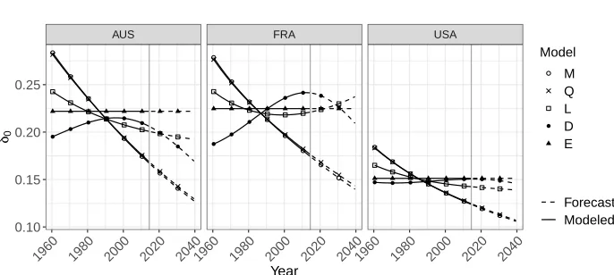
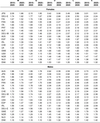
Table 1 shows the gains in life expectancy at birth produced by forecasting mortality with models M, Q, L, D, and E between 2015 and 2025 and between 2025 and 2035. For all countries and both sexes, the gains in life expectancy are forecast to be smaller with models M and Q than with the remaining three models. Models M and Q further lead to smaller gains ine0,tfor the period 2025–2035 than for the period 2015–2025. Figure 1
helps explain these results by showing the yearly changes in life expectancy produced by models M, Q, L, D, and E for three countries. A linear model of thelog(mx,t)(M) leads
Figure 1: Change in female life expectancy at birth over time (δ0), fitted and forecast with extrapolative models based on five (transformed) indicators for Australia, France, and the United States, 1960–2040
AUS FRA USA
1960 1980 2000 2020 20401960 1980 2000 2020 20401960 1980 2000 2020 2040 0.10
0.15 0.20 0.25
Year
δ0
Model
M Q L D E
Forecast Modeled
The other three models (L, D, and E) are generally more optimistic. Models L and D allow mixed patterns of life expectancy changes. That is, sometimes the increase in life expectancy accelerates (e.g., East Germany), sometimes it decelerates (e.g., Spain), and sometimes it alternates between acceleration and deceleration (e.g., France). In the long run, model E is often the most optimistic, due to its constant rate of increase. Life expectancy forecasts based onlx,t,dx,t,mx,t, andqx,twill compress against the last age
Table 1: Gains in life expectancy at birth for the periods 2015–2025 and 2025–2035 resulting from forecasting mortality with five models, females and males, 18 countries
M Q D L E
2015– 2025
2025– 2035
2015– 2025
2025– 2035
2015– 2025
2025– 2035
2015– 2025
2025– 2035
2015– 2025
2025– 2035
Females
JPN 2.09 1.88 2.15 1.95 3.42 3.06 3.49 3.86 3.01 3.01 DEU–E 1.74 1.62 1.77 1.67 2.58 2.68 2.30 2.50 2.24 2.24 FIN 1.67 1.52 1.70 1.56 2.44 2.34 2.31 2.43 2.21 2.21 FRA 1.66 1.52 1.69 1.55 2.38 2.27 2.24 2.30 2.25 2.25 ITA 1.66 1.50 1.69 1.53 2.33 2.19 2.27 2.31 2.55 2.55 PRT 1.62 1.45 1.64 1.47 2.14 2.02 2.23 2.18 3.23 3.23 AUT 1.61 1.46 1.63 1.49 2.18 2.08 2.10 2.12 2.31 2.31 DEU–W 1.58 1.45 1.60 1.48 2.20 2.14 2.07 2.12 2.19 2.19 AUS 1.58 1.42 1.59 1.44 2.00 1.86 1.99 1.95 2.22 2.22 ESP 1.54 1.35 1.56 1.37 1.98 1.76 2.05 1.97 2.58 2.58 IRL 1.52 1.39 1.54 1.41 1.97 1.93 1.91 1.92 2.15 2.15 CHE 1.51 1.37 1.53 1.40 2.12 1.98 2.03 2.05 2.06 2.06 UK 1.39 1.30 1.40 1.32 1.79 1.78 1.67 1.69 1.75 1.75 SWE 1.27 1.18 1.29 1.20 1.68 1.63 1.60 1.60 1.63 1.63 USA 1.20 1.12 1.20 1.13 1.50 1.49 1.42 1.40 1.51 1.51 NOR 1.15 1.08 1.17 1.10 1.48 1.49 1.42 1.44 1.47 1.47 NLD 1.12 1.06 1.14 1.08 1.47 1.47 1.37 1.38 1.38 1.38 DNK 1.09 1.04 1.10 1.05 1.53 1.61 1.35 1.39 1.32 1.32
Males
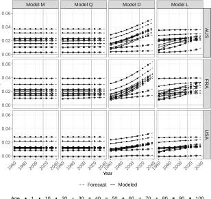
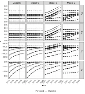
Figure 2 shows the fitted and forecastρx,t with models M, Q, L, and D for
Aus-tralia, France, and the United States. Theρx,twhen modeling and forecasting with model
M is constant in time but differs across ages. The constantρx,tis due to the use of the
log transformation and linear changes as shown in Table A-1 of Appendix A-2. With this model,ρx,tis generally lower at older ages due to relatively moderate decreases in
mortality observed at older ages compared with younger ages. As people keep surviving longer and thus dying at older ages, progress in life expectancy will become more depen-dent on mortality improvement at these ages. Asρx,tstays at lower levels at advanced
ages than at younger ages with this model, the decrease ofδ0,t over time observed in
Figure 1 is expected.
Figure 2: Fitted and forecast age-specific rate of mortality improvement (ρx) with four models based on the linear modeling of four transformed indicators for Australia, France, and the United States, females
ModelM ModelQ ModelD ModelL
A
U
S
F
R
A
U
S
A
1960 1980 2000 2020 20401960 1980 2000 2020 20401960 1980 2000 2020 20401960 1980 2000 2020 2040
0.00 0.02 0.04 0.06
0.00 0.02 0.04 0.06
0.00 0.02 0.04 0.06
Year
ρ
Forecast Modeled
For models Q, L, and D, ρx,t is increasing over time, at all ages. When life
ex-pectancy increase becomes dependent on mortality improvement at higher ages, progress in life expectancy would thus not necessarily be slowed down with these models but will depend, nevertheless, on how fastρx,tat older ages increases over time. We can thus
ex-pect that life exex-pectancy forecasts based on these models would be more optimistic than the forecasts based on a linear extrapolation oflog(mx,t).
The value ofρx,tfor model Q does change over time. However,ρx,tfor this model
stays relatively similar to theρx,tof model M. Despite changing rates of mortality
im-provement, the life expectancy forecasts using model Q remain more pessimistic than for models L and D.
Selecting a specific (transformed) indicator to forecast mortality thus affects the re-sults. Using a similar linear extrapolative model on the different (transformed) indicators leads to differences in life expectancy between 0.8 years (Danish males) and 6.1 years (Portuguese females) at the end of a 25-year forecast horizon (by 2040).
3.2 Which indicator gives the most accurate forecasts?
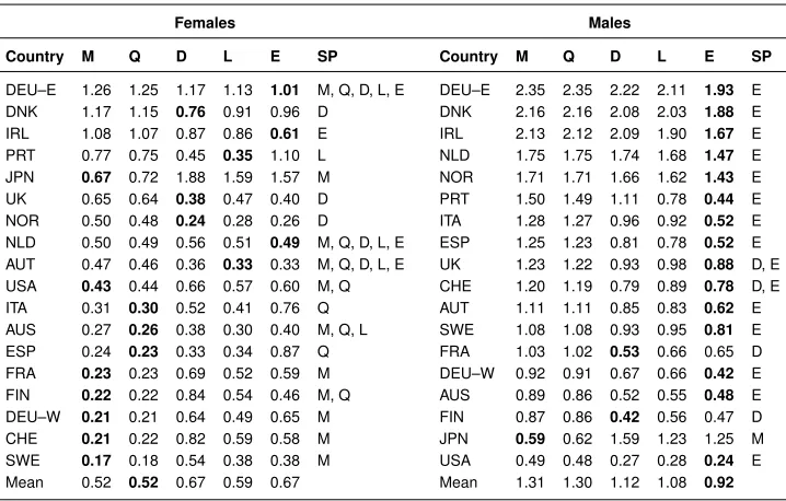
Table 2 shows the RM SE and the set of preferred models (SP), based on the MCS procedure, for life expectancy forecast by country and sex. The linear extrapolation of the
logit(qx,t)would have been, on average, the most accurate model for females. However,
model Q is only part of the SP for eight countries. Model M has the lowestRM SEh
statistics or no statistically different results from the best model (part of the SP) for 11 countries, model D for six countries, model L for five countries, and model E for four countries.
For males, life expectancy at birth over the period 1990–2014 would have been best predicted by the “optimistic” indicators, that is,lx,t,dx,t, ande0,t, for all countries, with
the exception of Japan. Model E would have been, on average, the most accurate model among those compared. Male life expectancy increased faster over this period, resulting from narrowing the gap with female life expectancy (Mesl´e 2004; Glei and Horiuchi 2007). Model E has the lowestRM SEhstatistics or no statistically different results from
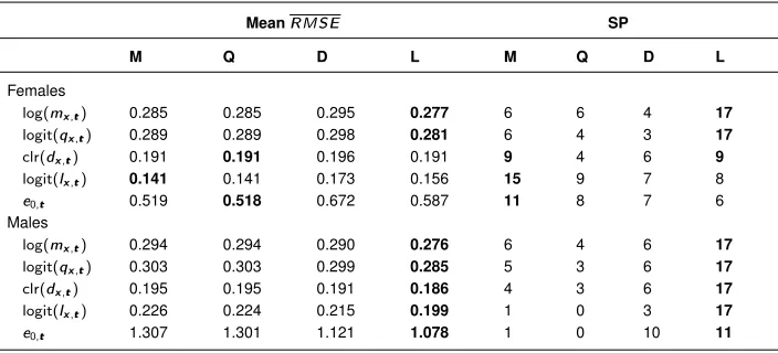
Table 2: Average root mean square error (RMSE) over forecast horizonhof the forecast life expectancy at birth for the period 1990 to 2014, with the bestRMSEvalue per country in bold and preferred set of models (SP) for 18 countries, females and males
Females Males
Country M Q D L E SP Country M Q D L E SP
DEU–E 1.26 1.25 1.17 1.13 1.01 M, Q, D, L, E DEU–E 2.35 2.35 2.22 2.11 1.93 E DNK 1.17 1.15 0.76 0.91 0.96 D DNK 2.16 2.16 2.08 2.03 1.88 E IRL 1.08 1.07 0.87 0.86 0.61 E IRL 2.13 2.12 2.09 1.90 1.67 E PRT 0.77 0.75 0.45 0.35 1.10 L NLD 1.75 1.75 1.74 1.68 1.47 E JPN 0.67 0.72 1.88 1.59 1.57 M NOR 1.71 1.71 1.66 1.62 1.43 E UK 0.65 0.64 0.38 0.47 0.40 D PRT 1.50 1.49 1.11 0.78 0.44 E NOR 0.50 0.48 0.24 0.28 0.26 D ITA 1.28 1.27 0.96 0.92 0.52 E NLD 0.50 0.49 0.56 0.51 0.49 M, Q, D, L, E ESP 1.25 1.23 0.81 0.78 0.52 E AUT 0.47 0.46 0.36 0.33 0.33 M, Q, D, L, E UK 1.23 1.22 0.93 0.98 0.88 D, E USA 0.43 0.44 0.66 0.57 0.60 M, Q CHE 1.20 1.19 0.79 0.89 0.78 D, E ITA 0.31 0.30 0.52 0.41 0.76 Q AUT 1.11 1.11 0.85 0.83 0.62 E AUS 0.27 0.26 0.38 0.30 0.40 M, Q, L SWE 1.08 1.08 0.93 0.95 0.81 E ESP 0.24 0.23 0.33 0.34 0.87 Q FRA 1.03 1.02 0.53 0.66 0.65 D FRA 0.23 0.23 0.69 0.52 0.59 M DEU–W 0.92 0.91 0.67 0.66 0.42 E FIN 0.22 0.22 0.84 0.54 0.46 M, Q AUS 0.89 0.86 0.52 0.55 0.48 E DEU–W 0.21 0.21 0.64 0.49 0.65 M FIN 0.87 0.86 0.42 0.56 0.47 D CHE 0.21 0.22 0.82 0.59 0.58 M JPN 0.59 0.62 1.59 1.23 1.25 M SWE 0.17 0.18 0.54 0.38 0.38 M USA 0.49 0.48 0.27 0.28 0.24 E Mean 0.52 0.52 0.67 0.59 0.67 Mean 1.31 1.30 1.12 1.08 0.92
Evaluating which indicators would have been the most accurate in predicting life expectancy is a complicated task as the results can change between countries, sexes, and periods. A trade-off between population forecast accuracy might be necessary in cases where more than one population is of interest, for example, losing accuracy for females to gain some for males. On average, for both sexes and all countries, model E would have been the most accurate model (RM SE= 0.79), followed by models L (RM SE= 0.83), D (RM SE = 0.90), Q (RM SE = 0.91), and M (RM SE = 0.91). When looking into the number of times a model is part of the preferred set (SP), for both females and males, model E still comes first (SP = 19), followed by models M (SP = 12), D (SP= 10), Q (SP= 8), and L (SP= 5).
Table 3: Average root mean square error (RMSE) over forecast horizon and country of the different transformed mortality indicators, with the bestRMSEvalue in bold, and number of times the model was part of the preferred set of models (SP), females and males
MeanRMSE SP
M Q D L M Q D L
Females
log(mx,t) 0.285 0.285 0.295 0.277 6 6 4 17
logit(qx,t) 0.289 0.289 0.298 0.281 6 4 3 17
clr(dx,t) 0.191 0.191 0.196 0.191 9 4 6 9
logit(lx,t) 0.141 0.141 0.173 0.156 15 9 7 8
e0,t 0.519 0.518 0.672 0.587 11 8 7 6 Males
log(mx,t) 0.294 0.294 0.290 0.276 6 4 6 17
logit(qx,t) 0.303 0.303 0.299 0.285 5 3 6 17
clr(dx,t) 0.195 0.195 0.191 0.186 4 3 6 17
logit(lx,t) 0.226 0.224 0.215 0.199 1 0 3 17
e0,t 1.307 1.301 1.121 1.078 1 0 10 11
4. Discussion and conclusion
This study is an overview of the implications the choice of life table statistic has for fore-casts. The results indicate that the LC type of models based onmx,tandqx,t
systemat-ically lead to more pessimistic forecasts than similar models based ondx,t,lx,tande0,t.
The choice of indicators is thus an important step when selecting a forecasting model, which can lead to important differences in the results.
The conclusions of the paper are generalizable to other populations, to other fitting periods, and for longer forecast horizons. Models M and Q will lead to more pessimistic forecasts than models D, L, and E for any population with decreasing mortality. The differences between models are, however, increasing with the forecast horizons. These conclusions arise as the pessimism of the forecasts of models M and Q seems to be rooted in the indicator and/or transformation used in these models, as further discussed in Section 4.1.
However, the conclusions of the paper might not be generalizable if the models are modified. Our models compare only simple linear extrapolation of the past trends for five (transformed) indicators, using a similar method. In practice, the models can, and sometime should, be modified to obtain better forecasts. For example, no modification has been made to model L to ensure that the forecastlx,tdecline monotonically with age.
models adapted to the acceleration or deceleration of rates of improvement over time exist and can better adapt to nonconstant rates of improvement (Bohk-Ewald and Rau 2017; Haberman and Renshaw 2012). Also, nonlinear extrapolation or adding covariates could potentially increase forecast accuracy (Raftery et al. 2013; Janssen, van Wissen, and Kunst 2013). Models considering the catch-up of laggards and coherence between populations have also shown potential (Li and Lee 2005; Hyndman, Booth, and Yasmeen 2013; Bergeron-Boucher et al. 2017; Pascariu, Canudas-Romo, and Vaupel 2018). Mod-ifications to the models could, and probably will, have an impact on the forecast results.
4.1 Why do the models produce different forecasts?
Given the similar methodology of models M, Q, D, L, and E, the difference between forecasts can be due to the use of a different indicator and the use of a different transfor-mation.
The effect of using one transformation rather than another is summarized in Ap-pendix A-2. The basic findings are that (1) the log transformation leads to a constant
ρx,tover time; (2) thelogittransformation allows for increasingρx,tover time that will
converge toward an upper limit; (3) the‘Brass’ logittransformation produces a changing
ρx,twith a limit of 0; and (4) the clr transformation allows for changingρx,tover time,
with no limit. The choice of transformation will thus have an impact on the forecast re-sults. For example, using alogittransformation ofmx,twill not lead to a constant rate
of improvement by age over time, as the log transformation does. However, a specific transformation cannot be applied to all indicators, as the transformation used should be adapted to the indicator’s characteristics. It is important to emphasise that only log-based transformations are compared in this paper. Other transformations are available, such as normal scores transformation, including the Wang transformation (e.g., de Jong and Marshall 2007). It is to be expected that the use of a normal scores transformation will provide different forecast results.
Quantifying the effect of choosing one indicator over another for the forecast results can be difficult. The relations between indicators in the life table are based on changes over ages (Preston, Heuveline, and Guillot 2001). However, when forecasting, the interest is also in changes over time. To estimate exactly how life table relations affect time changes, we need to know the relation over age between indicators (see Appendix A-5). For example, in the Lee and Carter (1992) model, we would need to know how the parametersαxandβxare changing over age (see equation (2)). These age patterns are
not linear and their modeling can be difficult as, for example,βxdoes not have a clearly
A-5 shows that life table relations modify the rates of mortality changes of indicators in the same set of life tables. For example, iflog(mx,t)are forecast linearly over time, log(lx,t)in the same life tables are not linear. The same modeling on different indicators,
for example, log-linear, would thus lead to different forecasts. Owing to the relations within the life table, modeling and forecasting an indicator in a certain way leads to different modeling of the other life table indicators and ultimately affects the trends in life expectancy.
4.2 Which indicator should be used for forecasting?
It has been established that basing a forecast on one indicator rather than another will have an impact on the results. However, the results do not provide us with a clear and universal guideline as to which indicator should be used to produce the most accurate forecast. The choice of indicator can depend on the purpose of the forecast, the research question, and the population of interest. Additionally, the results of the out-of-sample analysis in Section 3.2 are dependent on the fitting period, and the results might change if other data periods or longer forecast horizons were used for the analyis (see Appendix A-6).
Using life expectancy at birth as the forecasting indicator provides linear and steady forecasts. Model E is also more parsimonious in terms of parameters and tends to predict male life expectancy better than other models. However, this indicator does not provide any information about age distributions of mortality and provides less accurate forecasts for females when compared with the other models.
Models based on mx,t andqx,t are the most common, and the results show that
models M and Q tend to produce more accurate forecasts for females than other mod-els, especially for recent periods (Table 2). However, these models tend to overpredict mortality, especially for males or long forecast horizons (Appendix A-6).
Model L would have predicted the age and time patterns of mortality more accurately than the other age-specific models, in the recent past (Table 3). Model L has, however, a current shortcoming: This model does not ensure that thelx,tdecline monotonically with
age.
Table 4: Summary table
M Q D L E
Age-specific information Yes Yes Yes Yes No
ρx,t Constant Moderate Increase Increase
-δ0,t Decrease Decrease Mixed Mixed Constant
Interpretation
Progress in reducing age-specific death rates
Progress in reducing age-specific death probabilities
Lifesaving process
Improvement in survivorship
Increase in the expectation of life
4.3 Future directions
To forecast mortality, authors have used life expectancy (Pascariu, Canudas-Romo, and Vaupel 2018; Raftery, Lalic, and Gerland 2014; Raftery et al. 2013; Torri and Vaupel 2012; White 2002), life table deaths (Bergeron-Boucher et al. 2018, 2017; Oeppen 2008), and survival probabilities (Scherbov and Ediev 2016; Keyfitz 1991; de Jong and Marshall 2007). However, only a few models using these indicators are available, compared with models based on death rates and probabilities. Future studies should try to provide mod-els using life expectancy, life table deaths, and survival probabilities adapted to different contexts and populations, for example, forecasts for cohorts and by cause of death. Oep-pen (2008) and Kjærgaard et al. (2019) showed that the use of life table deaths provides interesting possibilities to forecast mortality by cause of death, due to the covariance structure between the components of compositional data. Survival probabilities are less prone to random fluctuations due to the cumulative nature of the indicator (from birth to agex), suggesting that their use could provide more robust forecasts.
Using death rates to forecast mortality has been the tradition so far, but other indica-tors can also be used. Each indicator can be derived from the others using life table rela-tions (except fore0,t) and provides insights about mortality in a population at a specific
point in time. Future developments in the field of mortality forecasting should consider the use of different indicators, but forecasters should bear in mind the implications of using a specific indicator for the forecast results.
5. Acknowledgments
References
Aitchison, J. (1986). The statistical analysis of compositional data. London: Chapman and Hall.doi:10.1007/978-94-009-4109-0.
Basellini, U. and Camarda, C.G. (2019). Modelling and forecasting adult age-at-death distributions. Population Studies 73(1): 119–138.
doi:10.1080/00324728.2018.1545918.
Bell, W.R. (1997). Comparing and assessing time series methods for forecasting age-specific fertility and mortality rates.Journal of Official Statistics13(3): 279–303. Bergeron-Boucher, M.-P., Canudas-Romo, V., Oeppen, J., and Vaupel, J.W. (2017).
Co-herent forecasts of mortality with compositional data analysis.Demographic Research
37(17): 527–568.
Bergeron-Boucher, M.-P., Simonacci, V., Oeppen, J., and Gallo, M. (2018). Coher-ent modeling and forecasting of mortality patterns for subpopulations using multiway analysis of compositions: An application to Canadian provinces and territories. North American Actuarial Journal22(1): 92–118.doi:10.1080/10920277.2017.1377620. Bernardi, M. and Catania, L. (2015). The Model Confidence Set package for R. Rine:
Tor Vergata University (Working Paper 362).doi:10.2139/ssrn.2692118.
Bohk-Ewald, C. and Rau, R. (2017). Probabilistic mortality forecasting with varying age-specific survival improvements. Genus73(1): 1–37.doi:10.1186/s41118-016-0017-8. Booth, H. and Tickle, L. (2008). Mortality modelling and forecasting: A review of
meth-ods. Annals of Actuarial Science3: 3–43.doi:10.1017/S1748499500000440.
Booth, H., Hyndman, R., Tickle, L., and de Jong, P. (2006). Lee–Carter mortality fore-casting: A multi-country comparison of variants and extensions. Demographic Re-search15(9): 289–310.doi:10.4054/DemRes.2006.15.9.
Booth, H., Maindonald, J., and Smith, L. (2002). Applying Lee–Carter under conditions of variable mortality decline. Population Studies 56(3): 325–336.
doi:10.1080/00324720215935.
Brass, W. (1971). On the scale of mortality. Taylor and Francis. London.
Cairns, A.J., Blake, D., and Dowd, K. (2006). A two-factor model for stochastic mortality with parameter uncertainty: Theory and calibration. Journal of Risk and Insurance
73(4): 687–718. doi:10.1111/j.1539-6975.2006.00195.x.
1–35.doi:10.1080/10920277.2009.10597538.
Carter, L.R. and Lee, R.D. (1992). Modeling and forecasting US sex differentials in mortality.International Journal of Forecasting8(3): 393–411.
de Jong, P. and Marshall, C. (2007). Mortality projection based on the Wang transform.
ASTIN Bulletin37(1): 149–161.doi:10.2143/AST.37.1.2020803.
Deb´on, A., Montes, F., and Puig, F. (2008). Modelling and forecasting mortality in Spain.
European Journal of Operational Research189(3): 624–637.
Ediev, D.M. (2008). Extrapolative projections of mortality: Towards a more consistent method part I: The central scenario. Vienna: Vienna Institute of Demography (Working Paper 03/2008).
Glei, D.A. and Horiuchi, S. (2007). The narrowing sex differential in life expectancy in high-income populations: Effects of differences in the age pattern of mortality. Popu-lation Studies61(2): 141–159. doi:10.1080/00324720701331433.
Gompertz, B. (1825). On the nature of the function expressive of the law of hu-man mortality, and on a new mode of determining the value of life contingen-cies. Philosophical Transactions of the Royal Society of London 115: 513–583.
doi:10.1098/rstl.1825.0026.
Haberman, S. and Renshaw, A. (2012). Parametric mortality improvement rate mod-elling and projecting. Insurance: Mathematics and Economics 50(3): 309–333.
doi:10.1016/j.insmatheco.2011.11.005.
Haldrup, N. and Rosenskjold, C.P.T. (2019). A parametric factor model of the term structure of mortality.Econometrics7(1).doi:10.3390/econometrics7010009. Hansen, P.R., Lunde, A., and Nason, J.M. (2011). The model confidence set.
Economet-rica79(2): 453–497.doi:10.3982/ECTA5771.
Hatzopoulos, P. and Haberman, S. (2013). Common mortality modeling and coherent forecasts. An empirical analysis of worldwide mortality data.Insurance: Mathematics and Economics52(2): 320–337.
HMD (2019). Human mortality database [electronic resource]. Berkeley: Uni-versity of California; Rostock: Max Planck Institute for Demographic Research
www.mortality.org.
Hyndman, R.J., Booth, H., and Yasmeen, F. (2013). Coherent mortality forecasting: The product-ratio method with functional time series models. Demography50(1): 261–
283.doi:10.1007/s13524-012-0145-5.
A functional data approach.Computational Statistics and Data Analysis51(10): 4942 – 4956.doi:10.1016/j.csda.2006.07.028.
Janssen, F., van Wissen, L.J., and Kunst, A.E. (2013). Including the smoking epidemic in internationally coherent mortality projections. Demography 50(4): 1341–1362.
doi:10.1007/s13524-012-0185-x.
Kannisto, V., Lauritsen, J., Thatcher, A.R., and Vaupel, J.W. (1994). Reductions in mor-tality at advanced ages: Several decades of evidence from 27 countries. Population and Development Review20(4): 793–810. doi:10.2307/2137662.
Keyfitz, N. (1991). Experiments in the projection of mortality. Canadian Studies in Population18(2): 1–17.doi:10.25336/P6C01S.
King, G. and Soneji, S. (2011). The future of death in America. Demographic Research
25(1): 1–38.doi:10.4054/DemRes.2011.25.1.
Kjærgaard, S., Ergemen, Y.E., Kallestrup-Lamb, M., Oeppen, J., and Lindahl-Jacobsen, R. (2019). Forecasting causes of death by using compositional data analysis: The case of cancer deaths.Journal of the Royal Statistical Society: Series C (Applied Statistics)
65(5): 1351–1370. doi:10.1111/rssc.12357.
Lee, R. (2000). The Lee–Carter method for forecasting mortality, with various extensions and applications. North American Actuarial Journal 4(1): 80–93.
doi:10.1080/10920277.2000.10595882.
Lee, R. and Miller, T. (2001). Evaluating the performance of the Lee–Carter method for forecasting mortality.Demography38(4): 537–549. doi:10.1353/dem.2001.0036. Lee, R.D. and Carter, L.R. (1992). Modeling and forecasting US
mortal-ity. Journal of the American Statistical Association 87(419): 659–671.
doi:10.1080/01621459.1992.10475265.
Li, H., O’Hare, C., and Zhang, X. (2015). A semiparametric panel approach to mortality modeling. Insurance: Mathematics and Economics 61(Supplement C): 264 – 270.
doi:10.1016/j.insmatheco.2015.02.002.
Li, N. and Lee, R. (2005). Coherent mortality forecasts for a group of popula-tions: An extension of the Lee–Carter method. Demography 42(3): 575–594.
doi:10.1353/dem.2005.0021.
Li, N., Lee, R., and Gerland, P. (2013). Extending the Lee–Carter method to model the rotation of age patterns of mortality decline for long-term projections. Demography
50(6): 2037–2051. doi:10.1007/s13524-013-0232-2.
Mathematical Geology35(3): 253–78.
Mesl´e, F. (2004). Life expectancy: A female advantage under threat. Population and Societies402(4): 1–4.
Oeppen, J. (2008). Coherent forecasting of multiple-decrement life tables: A test using Japanese cause of death data. Paper presented at the European Population Conference, Barcelona, Spain, July 10–July 12, 2008.
Oeppen, J. and Vaupel, J.W. (2002). Broken limits to life expectancy.Science296(5570): 1029–1031.doi:10.1126/science.1069675.
Pascariu, M., Canudas-Romo, V., and Vaupel, J.W. (2018). The double-gap life ex-pectancy forecasting model. Insurance: Mathematics and Economics78: 339–350.
doi:10.1016/j.insmatheco.2017.09.011.
Pawlowsky-Glahn, V. and Buccianti, A. (2011). Compositional data analysis: Theory and applications. Chichester: John Wiley and Sons. doi:10.1002/9781119976462. Pollard, J.H. (1987). Projection of age-specific mortality rates.Population Bulletin of the
United Nations(21/22): 55–69.
Preston, S., Heuveline, P., and Guillot, M. (2001). Demography: Measuring and model-ing population processes. Oxford: Blackwell Publishing.
Raftery, A.E., Chunn, J.L., Gerland, P., and ˇSevˇc´ıkov´a, H. (2013). Bayesian proba-bilistic projections of life expectancy for all countries. Demography50(3): 777–801.
doi:10.1007/s13524-012-0193-x.
Raftery, A.E., Lalic, N., and Gerland, P. (2014). Joint probabilistic projection of female and male life expectancy. Demographic Research 30: 795–822.
doi:10.4054/DemRes.2014.30.27.
Renshaw, A. and Haberman, S. (2006). A cohort-based extension to the Lee–Carter model for mortality reduction factors. Insurance: Mathematics and Economics38(3): 556 – 570.
Russolillo, M., Giordano, G., and Haberman, S. (2011). Extending the Lee–Carter model: A three-way decomposition. Scandinavian Actuarial Journal2011(2): 96–
117.doi:10.1080/03461231003611933. doi:10.1080/03461231003611933.
Scherbov, S. and Ediev, D. (2016). Does selection of mortality model make a dif-ference in projecting population ageing? Demographic Research 34(2): 39–62.
doi:10.4054/DemRes.2016.34.2.
doi:10.1186/s41118-018-0043-9.
Stoeldraijer, L., van Duin, C., van Wissen, L., and Janssen, F. (2013). Impact of dif-ferent mortality forecasting methods and explicit assumptions on projected future life expectancy: The case of the Netherlands. Demographic Research29(13): 323–354.
doi:10.4054/DemRes.2013.29.13.
Sweeting, P.J. (2011). A trend-change extension of the Cairns–Blake–Dowd model.
Annals of Actuarial Science 5(2): 143–162. doi:10.1017/S1748499511000017.
doi:10.1017/S1748499511000017.
Thatcher, R.A., Kannisto, V., and Vaupel, J.W. (1998). The force of mortality at ages 80 to 120. Odense: Odense University Press.
Torri, T. and Vaupel, J.W. (2012). Forecasting life expectancy in an international context.
International Journal of Forecasting28(2): 519–531.
Vaupel, J. and Yashin, A. (1987). Repeated resuscitation: How lifesaving alters life tables.
Demography24(1): 123–135. doi:10.2307/2061512.
White, K.M. (2002). Longevity advances in high-income countries, 1955–96.Population and Development Review28(1): 59–76. doi:10.1111/j.1728-4457.2002.00059.x. Wilmoth, J.R. (1990). Variation in vital rates by age, period, and cohort. Sociological
Methodology20: 295–335. doi:10.2307/271089.
Appendix
1. Identifiability and normalization
As pointed out by Lee and Carter (1992), an SVD does not provide a unique solution. A simple example is thatκtβxs= (−κt)(−βx)s. To obtain a unique solution for their
parameter estimates, Lee and Carter (1992) suggest normalizing κt andβx such that P
κ∗t = 0andP
βx∗ = 1, where∗ represents the parameter after normalization. The suggested normalization procedures by Lee and Carter (1992) are:
κ∗t =κt X
βxs, (6)
βx∗= Pβx
βx
. (7)
This normalizing procedure will not affect the estimate oflog(mx,t)−αx, asκtβxs=
κtPβxsPβx
βx. The parameters of the model (e.g., random walk with drift or linear
regression) used to fit and forecastκtare generally equivalent to those of a similar model
fitted toκ∗t. For example, if a random walk with drift is used, the drift (d) is calculated as:
d= κT−κ0
T −1 (8a)
d∗= κ
∗ T −κ∗0
T−1 =
Pβ
xs(κT−κ0)
T−1 =d
X
βxs. (8b)
This equivalence means that the continuous rates of mortality improvements (ρx,t=−log(mx,t+1) + log(mx,t)) are equivalent when usingκtorκ∗t:
−log(mx,(t+1)) + log(mx,(t)) =−[αx+ (κt+d)βxs] + [αx+κtβxs] =−dβxs
−log(mx,(t+1)) + log(mx,(t)) =−[αx+ (κ∗t+d ∗)β∗
x] + [αx+κ∗tβ ∗ x]
=−d∗βx∗=−[d X
βxs]
βx
P
βx
=−dβxs.
A similar proof can be made with a linear regression: if the parameters of the regression onκtareC0 andC1, those of a linear regression onκ∗t will be equal toC0Pβxsand
2. The transformation effect
Each of the mentioned transformations is adapted to the characteristic of a specific mor-tality indicator and cannot be applied to all indicators. For example, using a clr trans-formation of themx,twould lead to implausible results, as themx,t do not sum to a
constant nor represent parts of a whole. The log transformation of thedx,talso leads to
implausible results. The indicator is thus linked to a specific transformation. Even if each transformation is linked to a specific indicator, it is still possible to estimate how each transformation can affect the forecast results. To do so, we estimate the relative rates of mortality changer, with
rτt =−f˙
τ t
fτ
t
, (9)
wheref is a formula taking a linear form after transformationτ and the dot over the variable represents its derivative with respect to timet. The value ofrtindicates, similarly
toρx,t, where and how fast each function is changing over time.
In Table A-1,C0andC1are the coefficients of the linear regression. When modeling
and forecasting any indicator linearly after transformation, the following conclusions are drawn:
• The log transformation involves a constantr;
• Thelogittransformation involves a changingr, varying from0to−C1;
• The‘Brass’ logittransformation involves a changingr, varying fromC1to0;
• The clr transformation involves an increasingrover time, with no limit.
Hence, the transformations allow different progress in mortality, varying from constant changes to increase with no limit. It is important to note that for an equalC1, thelogit
transformation will be more pessimistic than the log transformation, asrtfor thelogit
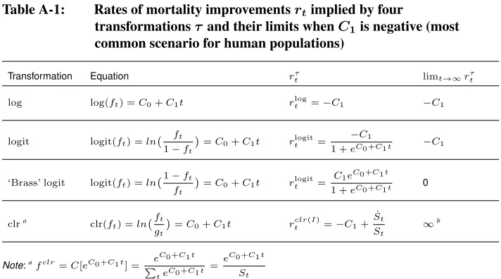
Table A-1: Rates of mortality improvementsrtimplied by four
transformationsτand their limits whenC1is negative (most common scenario for human populations)
Transformation Equation rtτ limt→∞rτt
log log(ft) =C0+C1t rtlog=−C1 −C1
logit logit(ft) =ln
ft 1−ft
=C
0+C1t rtlogit=
−C1
1 +eC0 +C1t −C1
‘Brass’ logit logit(ft) =ln 1−ft
ft =C
0+C1t rtlogit=
C1eC0 +C1t 1 +eC0 +C1t 0
clra clr(f
t) =ln ft
gt =C
0+C1t rtclr(I)=−C1+ ˙ St
St
∞b
Note:afclr=C[eC0 +C1t] = e C0 +C1t
P teC0 +C1t
= e
C0 +C1t
St
b
Theclrtransformation can only be used fordx,t, among the life table statistics. The general equation for
Stwhen forecastingdx,tisSt≈expD0 +D1t+D2t 2
. This equation provides a coefficient of determination above
99% for all countries and both sexes. Given this equation,rclr
t ≈ −C1+D1+ 2D2t. As the coefficientD2is
generally positive, the limit ofrclr
t will be∞.
3. Model confidence set (MCS)
The objective of the MCS procedure is to find the set of models or the model (M∗) that produces the most accurate forecast among the set of all considered models (M0). Using
the notation presented by Hansen, Lunde, and Nason (2011), that is identifying
M∗=i∈M0:µij≤0for allj ∈M0 ,
whereµij =E(cij,h)andcij,h=RM SEi,h−RM SEj,hfor alli,j= 1,. . .,m;iand
j are used to denote different models; andh = 1,. . .,H denotes the forecast horizon. The MCS procedure can be formulated using any loss function. In the current paper, we selected theRM SEhfunction.
The intuition behind the MCS procedure is: If the forecast accuracy differs between the models, the worst performing model is eliminated. The procedure is repeated until the hypothesis of equal predictive ability (H0,M : µij = 0,∀i,j) is accepted for all
remaining models inM, whereM is a subsetM0. It is necessary to define M as the
The relevant hypothesis to eliminate the worst performing models can be expressed as:
H0,M :µij = 0for alli,j = 1, 2,. . .,m
and the alternative hypothesis
HA,M :µij6= 0for alli,j= 1, 2,. . .,m.
We first definecij = PH
h=1cij,h
n andci =
P j∈Mcij
m . Hence, the test statistics are
defined as
tij =
¯
cij q
\
var(¯cij)
and ti = ¯
ci q
\
var(¯ci) ,
wherevar\(¯cij)andvar\(¯ci)are estimates of the variances of the defined averages. To test
the null hypothesisH0,M, Hansen, Lunde, and Nason (2011) consider the models with
the greatest relative loss by eliminating the worst performing model, that is the model with the largest test statistics. To do so, the following test statistics are defined and are used to define two elimination rules. The two test statistics are
TR,M = max
i,j∈M|tij| and Tmax,M = maxi∈Mti.
Note thatTR,M depends on the difference between two models whereasTmax,M
depends on the average over theith model. From these, the following eliminations rules are defined: emax,M = arg maxi∈MTmax,M andeR,M = arg maxi∈Msupj∈MTR,M.
4. Changes in life expectancy at birth
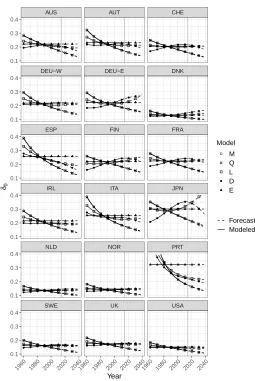
Figure A-1: Change in life expectancy at birth over time (δ0) fitted and forecast with extrapolative models based on five (transformed) indicators, 18 countries, females
● ● ● ● ● ● ● ● ● ● ● ● ● ● ● ● ● ● ● ● ● ● ● ● ● ● ● ● ● ● ● ● ● ● ● ● ● ● ● ● ● ● ● ● ● ● ● ● ● ● ● ● ● ● ● ● ● ● ● ● ● ● ● ● ● ● ● ● ● ● ● ● ● ● ● ● ● ● ● ● ● ● ● ● ● ● ● ● ● ● ● ● ● ● ● ● ● ● ● ● ● ● ● ● ● ● ● ● ● ● ● ● ● ● ● ● ● ● ● ● ● ● ● ● ● ● ● ● ● ● ● ● ● ● ● ● ● ● ● ● ● ● ● ● ● ● ● ● ● ● ● ● ● ● ● ● ● ● ● ● ● ● ● ● ● ● ● ● ● ● ● ● ● ● ● ● ● ● ● ● ● ● ● ● ● ● ● ● ● ● ● ● ● ● ● ● ● ● ● ● ● ● ● ● ● ● ● ● ● ● ● ● ● ● ● ● ● ● ● ● ● ● ● ● ● ● ● ● ● ● ● ● ● ● ● ● ● ● ● ● ● ● ● ● ● ● ● ● ● ● ● ● ● ● ● ● ● ● ● ● ● ● ● ● ● ● ● ● ● ● ● ● ● ● ● ● ● ● ● ● ● ● ● ● ●
SWE UK USA
NLD NOR PRT
IRL ITA JPN
ESP FIN FRA
DEU−W DEU−E DNK
AUS AUT CHE
1960 1980 2000 2020 20401960 1980 2000 2020 20401960 1980 2000 2020 2040
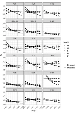
Figure A-2: Change in life expectancy at birth over time (δ0) fitted and forecast with extrapolative models based on five (transformed) indicators, 18 countries, males
● ● ● ● ● ● ● ● ● ● ● ● ● ● ● ● ● ● ● ● ● ● ● ● ● ● ● ● ● ● ● ● ● ● ● ● ● ● ● ● ● ● ● ● ● ● ● ● ● ● ● ● ● ● ● ● ● ● ● ● ● ● ● ● ● ● ● ● ● ● ● ● ● ● ● ● ● ● ● ● ● ● ● ● ● ● ● ● ● ● ● ● ● ● ● ● ● ● ● ● ● ● ● ● ● ● ● ● ● ● ● ● ● ● ● ● ● ● ● ● ● ● ● ● ● ● ● ● ● ● ● ● ● ● ● ● ● ● ● ● ● ● ● ● ● ● ● ● ● ● ● ● ● ● ● ● ● ● ● ● ● ● ● ● ● ● ● ● ● ● ● ● ● ● ● ● ● ● ● ● ● ● ● ● ● ● ● ● ● ● ● ● ● ● ● ● ● ● ● ● ● ● ● ● ● ● ● ● ● ● ● ● ● ● ● ● ● ● ● ● ● ● ● ● ● ● ● ● ● ● ● ● ● ● ● ● ● ● ● ● ● ● ● ● ● ● ● ● ● ● ● ● ● ● ● ● ● ● ● ● ● ● ● ● ● ● ● ● ● ● ● ● ● ● ● ● ● ● ● ● ● ● ● ●
SWE UK USA
NLD NOR PRT
IRL ITA JPN
ESP FIN FRA
DEU−W DEU−E DNK
AUS AUT CHE
1960 1980 2000 2020 20401960 1980 2000 2020 20401960 1980 2000 2020 2040
5. The indicator effect, an approximation
To understand how life table relations modify time trends,ρx,tfor different indicators are
analyzed after mortality is fitted and forecast with a baseline model (e.g., model M). This analysis can help explain how each indicator behaves under the same scenario, that is, in the same set of life tables. Unlike in the main text,ρx,tis calculated for all indicators
Ix,t:
ρx,t=−
Iˆx,t+1
ˆ
Ix,t
−1. (10)
Figure A-3 showsρx,tformx,t,qx,t,lx,tanddx,twhen mortality is fitted and
fore-cast with models M, Q, D, and L. Model M produces constantρx,tof mx,t. However,
this model produces a deceleration of survival improvements and changes in dx,tthat
converge toward a limit (see below). Similar results are found with model Q.
Theρx,tfor models L and D have different patterns than those for models M and
Q. Model L produces accelerating decline ofmx,t andqx,t, a deceleration of survival
improvement (less pronounced than that of model M), and changes indx,tthat also seem
to converge toward a limit. Model D produces accelerating decline ofmx,tandqx,t, a
deceleration of survival improvement, and accelerating changes indx,twith no apparent
limit.
Life table relations then do transform the time trends of indicators in the same set of life tables. Due to these relations, the same modeling on different indicators will not lead to the same forecast. For example, iflx,twould be forecast in a log-linear way, itsρx,t
Figure A-3: Rate of mortality changes for different indicators in a life table after mortality has been modeled with models M, Q, L, and D, Australian females, 1960–2040
Model M Model Q Model D Model L
m
x
t
q
x
t
d
x
t
l
x
t
1960 1980 2000 2020 20401960 1980 2000 2020 20401960 1980 2000 2020 20401960 1980 2000 2020 2040
0.00 0.01 0.02 0.03 0.04 0.05
0.00 0.01 0.02 0.03 0.04 0.05
−0.050 −0.025 0.000 0.025 0.050
−0.06 −0.04 −0.02 0.00
Year
ρ
Forecast Modeled
Age 1 10 20 30 40 50 60 70 80 90 100
To better understand how life table relations modify time trends, we can estimate life table functions in a continuous setting based on a specific model. We give an example for Model M. If we assume that the mortality age pattern follows a Gompertz model (Gompertz 1825) and assume that the force of mortality in a continuous setting, µx,t,
µx,t=αeβxevt. (11)
The life table identities of equation (11) are then found – that is,µx,tis transformed
into the others using standard life table relations – and the respective relative rate of mor-tality changertfor each indicator is calculated. Table A-2 shows the life table identities
and theirrt.
Table A-2: Life table formulas resulting from assuming thatµx,tis changing
exponentially over time, respective rate of mortality improvement
r, and limit ofrover time
Identities in the life table indicators
Assumption Converted tolx,t Converted todx,t
µx,t=αeβxevt lx,t=exp[
−α β (e
βx−1)evt] d
x,t=αexp[
−α β (e
βx−1)evt+βx+vt]
rµt =−v rtl=α
β(e
βx−1)evtv rd t =
α
β(e
βx−1)evtv−v
limt→∞rtl= 0 limt→∞rdt =−v
a
Note:a
Ifv <0in the original scenario, representing a decrease over time ofµx,t.
Ifµx,tis forecast assuming an exponential change, the correspondinglx,tdoes not
change exponentially (Table A-2). Thelx,tfor this scenario decelerates over time. Ifvis
negative in equation (11), the limit ofrl
tis 0. Asvis often negative in equation (11) for
human populations, representing a decrease ofµx,tover time, thenrtlof model M will
converge toward 0, representing a deceleration in survival improvements over time. Transformingµx,tintodx,tproduces an acceleration indx,tover time that will
con-verge toward−v (Table A-2). However, when comparingρx,tof model M with that of
model D, the latter will be more optimistic, asρx,tofdx,thas no limit (see Table A-1)
with this model.
In this analysis, only life table relations (Preston, Heuveline, and Guillot 2001) are used to transform one indicator into another. It is shown here that the relation over age between life table indicators transforms the time trends. The findings of Section 3 are then, at least partly, due the relations between indicators in the life table.
6. Forecast accuracy based on longer time periods
have data available since 1900, the analysis is limited to Denmark (DNK), France (FRA), Finland (FIN), Italy (ITA), the Netherlands (NLD), Norway (NOR), Sweden (SWE), and Switzerland (CHE). The results (Table A-3) differ from those in Section 3.2, especially for females. This illustrates the complexity of finding the most accurate forecast model for all populations and time periods.
Table A-3: Average root mean square error (RMSE) over forecast horizonhof the forecast life expectancy at birth for the period 1965 to 2014, with the bestRMSEvalue per country in bold and preferred set of models (SP) for eight countries, females and males
Females Males
Country M Q D L E SP Country M Q D L E SP
FIN 1.58 1.56 1.14 0.65 3.69 L FIN 2.59 2.58 2.32 1.35 1.56 L, E
ITA 1.40 1.37 0.70 0.37 4.07 L ITA 2.48 2.46 2.04 1.11 2.39 L
FRA 1.02 0.99 0.51 0.48 3.23 D, L NOR 1.97 1.96 1.85 1.38 1.48 L, E
DNK 0.88 0.87 0.83 0.95 2.57 M, Q, D,
L FRA 1.89 1.87 1.14 0.47 2.33 L NOR 0.83 0.82 0.60 0.35 2.81 L SWE 1.79 1.78 1.60 1.14 1.42 L, E
SWE 0.79 0.78 0.49 0.31 2.79 L CHE 1.73 1.70 1.03 0.83 1.34 D, L, E
CHE 0.66 0.63 0.63 0.76 3.01 M, Q, D,
L NLD 1.68 1.67 1.45 1.16 2.05
M, Q, D, L, E