Intensity Capping: a simple method to improve cross-correlation PIV results

R E S E A R C H A R T I C L E

Intensity Capping: a simple method to improve cross-correlation

PIV results

Uri ShavitÆRyan J. LoweÆJonah V. Steinbuck

Received: 2 September 2006 / Revised: 23 October 2006 / Accepted: 24 October 2006 / Published online: 15 December 2006 Springer-Verlag 2006

Abstract A common source of error in particle image velocimetry (PIV) is the presence of bright spots within the images. These bright spots are characterized by grayscale intensities much greater than the mean intensity of the image and are typically generated by intense scattering from seed particles. The displace-ment of bright spots can dominate the cross-correlation calculation within an interrogation window, and may thereby bias the resulting velocity vector. An efficient and easy-to-implement image-enhancement procedure is described to improve PIV results when bright spots are present. The procedure, called Intensity Capping, imposes a user-specified upper limit to the grayscale intensity of the images. The displacement calculation then better represents the displacement ofallparticles in an interrogation window and the bias due to bright spots is reduced. Four PIV codes and a large set of experimental and simulated images were used to evaluate the performance of Intensity Capping. The results indicate that Intensity Capping can significantly increase the number of valid vectors from experimen-tal image pairs and reduce displacement error in the analysis of simulated images. A comparison with other PIV image-enhancement techniques shows that

Inten-sity Capping offers competitive performance, low computational cost, ease of implementation, and min-imal modification to the images.

1 Introduction

A common problem in particle image velocimetry (PIV) studies is the appearance of bright spots in the images. The grayscale intensity of these bright spots is typically much higher than the mean intensity of the images. Bright spots may result from coalesced parti-cles, overlapping particles within the field of view, or individual particles located within highly illuminated regions (e.g., midway through the laser light sheet). In addition, many CCD cameras used in PIV experiments suffer from pixel anomalies (e.g., charge leakage), which may increase the intensity and total area of bright spots in an image.

Most PIV codes use the cross-correlation function to compute the particle displacements. The advantage of cross-correlation PIV over other methods, such as particle tracking velocimetry (PTV), is the relatively large sample size (number of particle pairs) that is used to calculate each velocity vector. A large number of particle pairs can increase the strength of the correla-tion peak, improving the deteccorrela-tion of the peak and reducing the uncertainty in the displacement calcula-tion (Raffel et al. 1998). For example, Keane and Adrian (1992) found that cross-correlation PIV requires more than five particle pairs within the inter-rogation window to yield a valid vector detection probability higher than 95%. However, if bright spots U. Shavit (&)

Civil and Environmental Engineering, Technion, Haifa 32000, Israel

e-mail: [email protected]

R. J. LoweJ. V. Steinbuck

are present in the images, the cross-correlation may be dominated by a small number of high-intensity pixels. As a result, the number of particle pairs that contribute to the cross-correlation peak may be small (<5). Fur-thermore, if the displacement of the bright spots differs from the mean particle displacement within a subwin-dow (e.g., in sheared or turbulent flows), then the resulting velocity vector may be spurious.

A common approach for removing spurious vectors is to employ filtering techniques after the cross-correlation analysis. The rejected vectors are then replaced using interpolation based on kernel weight functions, typically of 8 or 24 neighboring vectors. Since filtering techniques may not detect all of the spurious vectors and since interpolation introduces unknown errors, it is desirable to minimize the generation of spurious vectors.

In order to minimize the occurrence of spurious vectors in PIV results, two approaches are often implemented: PIV algorithm improvement and image enhancement prior to PIV processing. The symmetric phase only filtering (SPOF) technique is an example of PIV algorithm improvement (Wernet 2005). This technique modifies the FFT procedure by adding a normalized filter such that only the phase contributes to the cross-correlation result. Image-enhancement techniques, such as the one presented in this paper, do not necessitate modifications to the PIV algorithm since they are applied prior to PIV processing. West-erweel (1993) proposed a min/max image-enhance-ment technique that minimizes variations in the recorded particle image intensities and reduces back-ground noise. Dellenback et al. (2000) modified their low quality PIV images by applying enhancement techniques such as thresholding, contrast enhance-ment, histogram equalization, and histogram hyperb-olization. Roth and Katz (2001) developed a modified histogram equalization (MHE) technique that com-bines thresholding and histogram stretching. Fore et al. (2005) enhanced their PIV images by subtracting a background image (obtained by averaging a series of images) and then linearly stretching the grayscale range. Notably, each of these techniques fully re-maps the images by replacing the original intensity of each pixel with a new value. Thus, care must be taken to avoid image modifications that degrade the accuracy of the PIV results.

In this paper, we provide an image-enhancement procedure for improving PIV results when bright spots are present in the images. The procedure only affects a small number of pixels in the images and thereby limits potentially harmful image modifications. The improvement is achieved by applying an upper limit to

the grayscale values of the images. This image enhancement, called Intensity Capping, is performed before the image pair is analyzed using the cross-cor-relation. As such, it can be applied when using either commercial or open-source PIV codes. Being a simple modification to the images, Intensity Capping is com-putationally cheap and easy to implement.

2 Methodology

2.1 Description of Intensity Capping

To explain Intensity Capping, we examine an interro-gation window containing particles that move a dis-tance dx between subsequent images. The first grayscale image is described by f and the second is described byg. The two-dimensional cross-correlation of the images is given by

/_fgðmÞ ¼

Z

fðx0þmÞgðx0Þdx0; ð1Þ

where x¢ is the spatial variable, m is the shift in the correlation plane, and bold indicates two-dimensional variables. The limits of integration will depend on the size of the interrogation window. The two-dimensional particle displacement, dx, is identified by the spatial location of the cross-correlation maximum:

/_fgðdxÞ ¼maxð/_fgðmÞÞ: ð2Þ

Suppose now that the first and second images,fand

g, contain bright spots with intensities that are much greater than the mean intensity of the images. We decompose image f as f = f1 + f2 and image g as g = g1 +g2, where the subscript ‘‘1’’ indicates the

image without the bright spots and the subscript ‘‘2’’ indicates the imaged bright spots. Substituting these decomposed forms for fandginto Eq. 1 gives /_fgðmÞ ¼/_f1g1ðmÞ þ/_f1g2ðmÞ þ/_f2g1ðmÞ þ/_f2g2ðmÞ;

ð3Þ

where

/_f1g1ðmÞ ¼

Z

f1ðx0þmÞg1ðx0Þdx0; ð4aÞ

/f1g2ðmÞ ¼

Z

f1ðx0þmÞg2ðx0Þdx0; ð4bÞ

/f2g1ðmÞ ¼

Z

/_f2g2ðmÞ ¼

Z

f2ðx0þmÞg2ðx0Þdx0: ð4dÞ

Finally, substitution of Eq. 3 into Eq. 2 yields the equation for the particle displacement,

/fgðdxÞ ¼max /f1g1ðmÞ þ/f1g2ðmÞ

þ/_f2g1ðmÞ þ/_f2g2ðmÞ ð5Þ

Assuming the number of bright spots in the inter-rogation window is small, /f1g1(m) represents the

contribution of the majority of the particles to the total cross-correlation,/fg (m). The remaining three terms, /f1g2(m)/f2g1(m) and/f2g2(m), represent the

contri-bution to the cross-correlation by the small number of bright spots. Note that the bright spots correlate both with themselves and with the particles of moderate intensity. Since the intensities off2andg2are high, the

contribution to the correlation by bright spots can be significant, if not dominant. The calculated displace-ment may then depend on the correlations of the bright spots. If the bright spots do not follow the local flow then/fg(m) may be biased and spurious vectors may result.

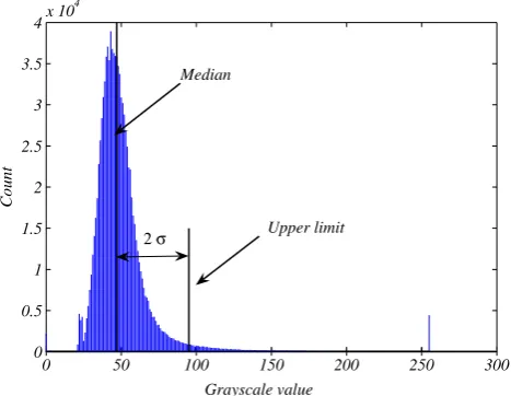
To ameliorate this problem, we propose to impose an upper limit on the grayscale values of all the pixels in images f and g. As illustrated in Fig.1, the upper limit can be expressed as I0 + nrI, where I0 is the

grayscale median intensity of the image, rI is the standard deviation of the intensity, and n is a user-specified constant (e.g., n = 2 in Fig.1). Pixels with grayscale intensities higher thanI0+ nrIare replaced

by this grayscale value (i.e., the valueI0+ nrI); all of

the other pixels are left unchanged. As a result of this Intensity Capping, the intensity values inf2andg2are

reduced substantially and the contributions of /f1g2

(m),/f2g1(m), and/f2g2(m) to/fg(m) are diminished. Consequently, the calculated displacement, dx, in Eq. 5 will better reflect the average displacement ofall

particles in the interrogation window and will be less biased towards the displacement of bright spots. 2.2 Application of Intensity Capping to PIV images The performance of Intensity Capping is evaluated for both experimental images (Sect. 3) and synthetic ima-ges (Sect.4). Capped image pairs were processed using four different cross-correlation PIV codes: MatPIV 1.6.1 (Sveen 2004); UraPIV (Gurka et al. 1999); Vid-PIV 4.0 g (ILA, Juelich, Germany, 2001); and Insight 6.0 (TSI, Shoreview, MN, 2005). The first two codes were developed using Matlab (Mathworks) and are open-source. The second two codes are commercially distributed. We emphasize that we do not seek to compare the effectiveness of these PIV codes, but rather seek to evaluate the performance of Intensity Capping for a broad set of PIV algorithms.

In all of the PIV analysis, interrogation windows of 32·32 pixels with 50% overlap were used, yielding velocity vectors every 16 pixels. When using UraPIV, VidPIV, and Insight, only a single cross-correlation pass (iteration) was performed. However, a multiple-pass algorithm was implemented when using MatPIV. In the first pass, an interrogation window of 64·64 pixels was used to calculate the particle dis-placements. The displacement results were then used to locate the center of the interrogation window in the second pass. Two more passes, using 32· 32 pixel windows, were used to generate the final velocity vector maps.

In Sect.3, the performance of Intensity Capping is analyzed using a set of experimental images. For each image pair, intensity capped images were generated by assigning pixels with an intensity exceeding I0+ nrI,

with the valueI0+ nrI. In order to identify the value

ofnthat yielded the greatest improvement to the PIV results, Intensity Capping was applied for a range of different n values (i.e., –0.1 to either 11 or 40, depending on the image pair). For these experimental image pairs, the true velocity field is not known. Therefore, in order to assess the effect of Intensity Capping, a local consistency filter was used to quantify the change in the number of valid vectors. Those velocity vectors (u and v) within two standard devia-tions of the median of their 24 (=52–1) neighbors were

0 50 100 150 200 250 300 0

0.5 1 1.5 2 2.5 3 3.5

4x 10

4

Grayscale value

Count

Median

Upper limit

2 σ

considered valid, while those outside this range were marked as outliers. This filter range appeared appro-priate for the velocity maps considered here. It is important to emphasize that the number of valid vec-tors can be a function of both the performance of the PIV codes and the quality of the images. Thus, in order to evaluate Intensity Capping, we are strictly interested in the relative improvement (i.e., reduction of spurious vectors) obtained by each code for each individual experiment.

In Sect.4, a series of synthetic images are used to evaluate the performance of Intensity Capping for various flow conditions (turbulence, shear, and cross-plane motion) and image characteristics (particle seeding density and peak particle intensity). These images were capped either at specific intensity values (ranging from 1 to 3,500) or by using the same proce-dure as applied for the experimental images. Using synthetic images, it is possible to directly quantify the effect the Intensity Capping by comparing capped PIV results to the known, true velocity field. In the evalu-ation of the synthetic image trials, only MatPIV was used for the PIV processing.

2.3 Comparison with other image-enhancement techniques

In Sects.3and4, results obtained by Intensity Capping are compared to three alternative image-enhancement algorithms. The first image-enhancement technique considered is MHE (Roth and Katz 2001). MHE was implemented as described by Roth and Katz (2001), with the exception that the entire image was used as a single tile. This change had little effect on the MHE results since the images do not suffer from reflections from solid surfaces and their illumination is relatively uniform. This technique involves varying a parameter,

x, which describes the percent area of the image that does not contain particles. The MHE algorithm was applied to each image pair using a range of differentx

values. The velocity field corresponding to the value of

xgiving the least number of spurious vectors was then selected for comparison with Intensity Capping.

The second image-enhancement algorithm consid-ered is the min/max technique (Westerweel1993). In this procedure, the grayscale value of each pixel is modified as follows,

Imðx;yÞ ¼Imax

Iðx;yÞ minðItileÞ

maxðItileÞ minðItileÞ

; ð6Þ

whereIm (x,y) is the new, modified grayscale value of

pixel (x,y),I(x,y) is the original grayscale value of pixel

(x,y), Imax is the maximum possible image intensity

(e.g., 255 for 8-bit images and 4,095 for 12-bit images) and Itile is the intensity array of user-specified size,

centered about pixel (x,y). Following Westerweel (1993), we first computed the minimum and maximum values ofItileover the entire image and then applied a

uniform, moving-average filter with a template size equal to the tile size to generate the values of min(Itile)

and max(Itile). To avoid a nearly zero denominator in

Eq. 6, we did not apply min/max for the condition max (Itile) – min (Itile) < 10. The optimum tile size depends

on characteristics of the image pair, including particle image size and spatial variations in the image back-ground. For this study we evaluated the min/max technique for a range of tile sizes: 5·5, 9· 9, 15·15 and 25·25 pixels.

The final image-enhancement algorithm used for comparison is contrast limited adaptive histogram equalization (CLAHE), as implemented using ‘adapthisteq.m’ in the Matlab Image Processing Tool-box, Mathworks, Inc. The CLAHE function was applied using the default setting (full grayscale range of the original images, tiles of 8 · 8 pixels, and a uni-form histogram shape) with no further tuning.

3 Evaluation of experimental PIV images

3.1 Experimental images

Six experimental image pairs were evaluated (Table1). ‘‘Flume_1’’ (Rosenzweig 2005), ‘‘Wave_1’’ (Shavit et al.2003), and ‘‘Air’’ (Gurka1999) were obtained at the Technion (Israel Institute of Technology, Haifa, Israel). ‘‘Ocean’’ was obtained by the Marine Physical Laboratory, Scripps Institution of Oceanography, University of California, San Diego. ‘‘Flume_2’’ and ‘‘Wave_2’’ (Lowe 2005) were obtained at the Envi-ronmental Fluid Mechanics Laboratory, Stanford University. These six image pairs represent a wide range of flows, environmental conditions (e.g., labora-tory and field, water and air), acquisition systems (e.g., laser power and camera bit-depth), and image char-acteristics.

Barbara Channel Islands, California. The ‘‘Air’’ image pair was acquired in the near-exit region of an air jet that injected seeded air into stagnant, un-seeded air. Both ‘‘Ocean’’ and ‘‘Air’’ contain some regions of low seeding density due to the challenges associated with natural seeding (low particulate con-centrations) and due to the un-seeded stagnant air, respectively. The last two columns of Table1 provide the values of the grayscale median, I0, and standard

deviation, rI, of the original (uncapped) images for each experiment.

3.2 Results from experimental images

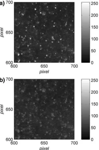
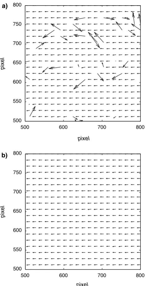
Figure2 shows an example image (‘‘Flume_1’’, 1st image) before and after the application of Intensity Capping (~1% of the image area is shown). The upper limit grayscale intensity value used to cap the image was equal to I0+ 2rI (Fig.1). A comparison of the two images shows that Intensity Capping eliminates the bright spots, while preserving the rest of the image. Note that the particles that produced the bright spots are still present in the capped image but appear with reduced intensity. Figure3 shows the resulting unfiltered PIV results for both the original (uncapped) and capped image pairs (covering~10% of the image area). Figure3 demonstrates that Intensity Capping significantly reduces the number of outliers for this image pair.

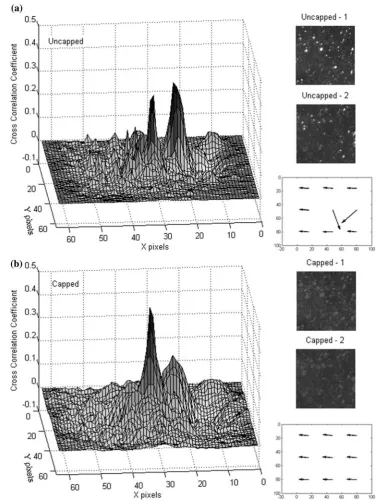
Figure 4 shows cross-correlation maps for a single interrogation region from ‘‘Flume_1’’. These maps correspond to the center vector of the nine vectors shown in Fig.4a (uncapped) and b (capped). In the uncapped case (Fig. 4a), two dominant correlation peaks are observed: the true peak associated with the net particle motion (left) and a spurious peak associ-ated with the presence of bright spots (right). The application of Intensity Capping effectively reduces the height of the spurious peak and increases the height of the true cross-correlation coefficient peak (Fig.4b). It should also be noted that the application of Intensity Capping acts to reduce intensity at particle centers (i.e., it makes particle intensity profiles look more like top-hat functions) and thus the width of the true cor-relation peak may broaden.

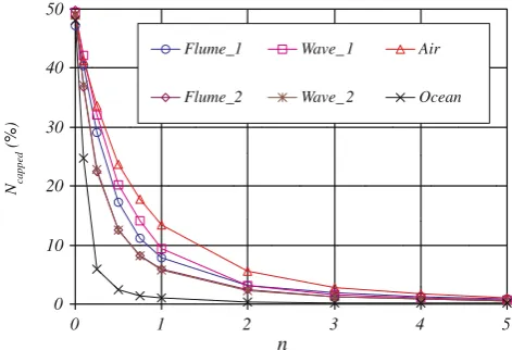
Figure 5shows the Intensity Capping results at dif-ferent values ofn, calculated using MatPIV for each of the experimental image pairs. The results obtained using the other three codes (not shown) were qualita-tively the same. Intensity Capping increases the per-centage of valid velocity vectors for each of the image pairs, with no exception. As n declines from nearly

Table 1 Technical specifications for each of the six experimental image pairs used to evaluate Intensity Capping

Image pair Camera Bits Image size Seed I0 rI

Flume_1 Kodak MegaPlus ES1.0 8 1030 · 992 GS 47/45 23/19

Wave_1 Kodak MegaPlus ES1.0 8 1030 · 992 GS 56/61 19/16

Air Kodak MegaPlus ES1.0 8 1030 · 992 PG 22/22 35/35

Ocean Cooke, CCD Sony ICX385 12 1040 · 1376 NT 65/64 23/25

Flume_2 Redlake MegaPlus ES4.0/E 12 2048 · 2048 GS 82/78 78/65

Wave_2 Redlake MegaPlus ES4.0/E 12 2048 · 2048 GS 64/68 56/66

I0is the grayscale median andrIis the grayscale standard deviation of the first and the second images in each pair.dpis the diameter of the seed particles. The following seeding particles were used:GShollow glass spheres made by Potters Industries (dp11lm);PG propylene glycol droplets (dp< 1lm);NTnatural ocean seeding (suspended sediment, phytoplankton, and zooplankton) at approx-imately 40 m depth

uncapped values (e.g.,n~11 to 40), Intensity Capping exhibits improving performance, until a threshold value is achieved (n~0 to 3) at which the PIV results rapidly degrade. Improved results are obtained for smallernbecause bright spots are capped to a greater extent. At very lown values (n ~ 0), the image signal level (i.e., particle intensity) approaches the back-ground noise and thus the results degrade. Figure5 shows that a choice ofn = 0.5–3 yields the best PIV

results. Further investigation of these experiments re-veals that the optimalnvalue (based on the analysis of a subset of images) is typically valid for the entire set of images.

Table 2 summarizes the Intensity Capping results for combinations of the experimental image pairs and PIV codes. P0represents the percentage of valid

vec-tors in the original (uncapped) images.Pbestrepresents

the highest percentage of valid vectors obtained using Intensity Capping. ‘‘Improvement’’ describes the rela-tive change in the percentage of valid vectors due to Intensity Capping, i.e., (Pbest – P0)/P0· 100. Lastly, nbest is the value of n used to generate Pbest. The

absolute percentage of valid vectors, P0andPbest, are

dependent on the quality of the original images and PIV code performance and thus do not necessarily reflect the performance of Intensity Capping. For example, a camera defect left a thin, black (zero intensity) strip at the bottom of the ‘‘Flume_1’’, ‘‘Air’’, and ‘‘Wave_1’’ images. ‘‘Flume_1’’ and ‘‘Air’’ images were processed with the strip intact, while ‘‘Wave_1’’ was processed after the strip was removed. As a result, both P0 and Pbest are higher for ‘‘Wave_1’’ than for

‘‘Flume_1’’ and ‘‘Air’’. Therefore, it should be stressed that the relative improvement, not the absolute per-centage of valid vectors (P0andPbest), is the relevant

parameter for evaluating the performance of Intensity Capping.

The relative improvement in valid vectors due to Intensity Capping ranges from 1.6 to 11.1% (Table2). The ‘‘Ocean’’ PIV results show the greatest improve-ment (11.1%) of all of the experiimprove-ments (Table2). The relatively narrow intensity histograms of the ‘‘Ocean’’ images (rI= 23/25 for 12-bit, Table1) suggest that the uncapped images may be highly susceptible to PIV biases due to bright spots. Since the intensity variance in the images is small, bright spots make a large con-tribution to the cross-correlation and may thereby generate PIV outliers. This is exhibited in the relatively low absolute percentage of valid vectors (P0= 86.1%).

In the absence of bright spots (i.e., for the intensity capped images), the ‘‘Ocean’’ images yield a high percentage of valid vectors (Pbest= 96%).

The average improvement is somewhat higher for images that were generated by 12-bit cameras (i.e., ‘‘Ocean’’, ‘‘Flume_2’’, and ‘‘Wave_2’’) than for those generated by the 8-bit camera (i.e., ‘‘Air’’, ‘‘Flume_1’’, and ‘‘Wave_1’’). This result is expected since the grayscale intensity of a bright spot may be 16 times larger in a 12-bit camera than in an 8-bit camera. As the median and standard deviation of the grayscale intensities of the six image pairs are within the same order of magnitude (see Table1), a bright spot in a

500 600 700 800

500 550 600 650 700 750 800

pixel

pixel

500 600 700 800

500 550 600 650 700 750 800

pixel

pixel

a)

b)

12-bit image is likely to have a greater influence on the cross-correlation than a bright spot in an 8-bit image.

Notably, Intensity Capping also improves PIV re-sults for images that contain bright spots due to bad pixels on the CCD array. Damaged pixels (e.g., anomalously sensitive or saturated pixels) are common and their number may increase with camera age. The cross-correlation is likely to be dominated by damaged pixels that appear with the maximum possible value (e.g., 255 in 8-bit images). Images ‘‘Flume_1’’, ‘‘Wave_1’’ and ‘‘Air’’ have about 25 bad pixels (with a

grayscale value of 255) that generate ~10 spurious vectors in each velocity field. Since the number of bad pixels in each interrogation window is relatively small, Intensity Capping reduces the influence of these sta-tionary bad pixels and produces accurate velocity vectors in these regions. Note that when bad pixels appear in the same location in every image, other techniques such as background subtraction could be used to prevent spurious vectors. However, if bad pixels arise erratically in space or time, Intensity Capping is likely to be a superior solution.

Fig. 4 Cross-correlation coefficient maps of one subwindow (32·32 pixels) in ‘‘Flume_1’’ before and after the application of Intensity Capping. The image

subwindows and displacement results (shown in pixel coordinates) on the right cover a pixel area of 368 <x< 464 and 752 <y< 848. The cross-correlation coefficient maps correspond to the vector in the center of the displacement field. The results were obtained using MatPIV with two passes with no

In Table2, the results obtained with three existing image-enhancement techniques (described in Sect.2.3) are compared to those obtained with Intensity Capping. The level of improvement obtained using the MHE method is comparable, but slightly lower than that obtained by Intensity Capping for all of the experiments. It should be noted that for their particular

images, Roth and Katz (2001) found thatx = 94% gave the best results, while the bestxvalues for our images varied between 40 and 65% for the 12-bit images and between 5 and 10% for the 8-bit images. For min/max, values cited in Table2 represent the best results ob-tained among the four different tile sizes evaluated. These correspond to tile sizes of 9, 9, 25, 15, 9, and 9 for images ‘‘Flume_1’’, ‘‘Wave_1’’, ‘‘Air’’, ‘‘Ocean’’, ‘‘Flume_2’’ and ‘‘Wave_2’’, respectively. In most cases, the min/max technique significantly improves the results, but the percentage of valid vectors was lower than obtained using Intensity Capping. The application of min/max to the ‘‘Air’’ trial was one exception, in which a slight degradation resulted for all tile sizes. This may have been caused by the variable seeding density near the edges of the jet (see Sect.3.1) The CLAHE function generally improves the results and performs slightly better than MHE, min/max and Intensity Capping. However, instead of improving the ‘‘Ocean’’ PIV results, CLAHE reduces the number of valid vectors from 86.1% in the original image pair to 82.5% in the enhanced images. It seems that the CLAHE algorithm is unable to effectively re-map the narrow intensity histogram of the ‘‘Ocean’’ images.

The relatively small modification to the images is another advantageous feature of Intensity Capping. While MHE, min/max, and CLAHE re-map the entire

86 88 90 92 94 96 98 100

-5 0 5 10 15 20 25 30 35 40

Flume_1 Wave_ 1 Air_jet

Flume_2 Wave_ 2 Ocean

V

a

lid

v

elocit

y

v

ector

s (

%)

n

Fig. 5 The percentage of valid velocity vectors as a function of the number of standard deviations,n, used for the definition of the Intensity Capping upper limit. These results were obtained using MatPIV. The PIV results are optimal fornbetween 0 and 3. Asnapproaches zero (i.e., the upper limit nears the grayscale median), the number of valid vectors decreases sharply. In the opposite limit, as n becomes large, the percentage of valid vectors asymptotes to its uncapped value

Table 2 The results of the analysis of experimental images

P0 Pbest Improvement (%) nbest Ncapped(%) MHE min/max CLAHE

Flume_1

MatPIV 87.2 93.7 7.5 3 1.8 93.3 92.4 94.0

VidPIV 88.8 94.9 6.8 3 1.8 – – 95.5

URAPIV 86.5 93.0 7.5 3 1.8 – – 94.3

TSI 89.5 94.6 5.8 2 3.0 – – 95.2

Wave_1

MatPIV 96.0 98.0 2.1 2 3.2 96.8 97.4 98.3

VidPIV 93.1 96.3 3.4 3 1.6 – – 97.0

URAPIV 93.9 96.5 2.8 2 3.2 – – 97.6

TSI 93.5 96.9 3.7 3 1.6 – – 97.2

Air

MatPIV 93.4 94.9 1.6 1 13 94.7 92.8 95.0

VidPIV 90.7 94.9 4.7 1 13 – – 95.4

URAPIV 91.3 93.8 4.2 2 5.6 – – 94.8

TSI 90.2 94.6 4.9 1 13 – – 95.0

Ocean

MatPIV 86.1 96.0 11.1 0.5 2.2 95.3 91.4 82.5

Flume_2

MatPIV 92.3 97.5 5.6 2 2.4 97.0 97.3 98.7

Wave_2

MatPIV 91.5 97.4 6.5 2 2.3 96.6 97.2 97.4

image and change the grayscale value of each pixel, Intensity Capping improves the PIV results by chang-ing only a small fraction of the total number of pixels. Table2 shows the percentage of pixels that were changed by Intensity Capping,Ncapped, whenPbestwas

obtained. Figure6 shows that for all of the experi-mental image pairs, with the exception of the ‘‘Air’’ case, the number of changed pixels is less than 3.2% for

n= 2, and less than 1.8% forn= 3. Thus, the best PIV results for each experiment are generally obtained while leaving at least 96.8% of the pixels unchanged. The relatively high values of Ncapped for the ‘‘Air’’

image pair are related to the low median intensity value (I0= 22, Table 1) caused by the unseeded

re-gions that appear on both sides of the air jet. Figure6 also shows that the ‘‘Ocean’’ experiment, which shows the greatest improvement due to Intensity Capping, actually has the lowest fraction of pixels changed. Considered together, Figs.5and 6indicate that a sig-nificant improvement in PIV results can be achieved with a very small modification to the images.

In addition to the aforementioned image-enhance-ment techniques, the performance of the symmetric phase only filtering (SPOF) algorithm modification (Wernet 2005) was also evaluated. The SPOF tech-nique was selected for comparison because, like Intensity Capping, it is computationally inexpensive. We found that SPOF did not improve the PIV results for the set of experimental image pairs. While SPOF yields more accurate velocities for images containing DC background noise and low signal-to-noise ratio (SNR) cross-correlations (Wernet 2005), it appears that it is not well-suited to remedy displacement biases from bright spots characterized by high spatial fre-quency and high SNR cross-correlations. For PIV

images containing both DC background noise and bright spots, we hypothesize that a combined approach involving both SPOF and Intensity Capping may be fruitful.

4 Evaluation of synthetic PIV images

4.1 Synthetic image generator

Simulated images have been used in many PIV anal-yses (Keane and Adrian 1992; Westerweel 1993; Cowen and Monismith 1997). Our image generator follows closely from the models described in Raffel et al. (1998) and Cowen and Monismith (1997).

Particles were randomly assigned a location within a simulated light sheet, using a uniform distribution. The particle seeding density was held fixed (except when explicitly varied), to an average of 15 particles/sub-window (32 pixels·32 pixels). The particle locations in the first image were held constant for each set of trials to prevent variations in PIV results due to ran-dom particle placement. The particles were then sub-jected to a specified displacement prior to the generation of the second image.

A peak intensity, Ip, was specified for each particle

located within the laser light sheet (|Z| < 1/2DZ0,

whereZis each particle’s cross-plane location andDZ0

is the light sheet thickness). The light sheet profile was assumed to be Gaussian (Raffel et al.1998), i.e.,

IpðZÞ ¼qexp Z2. ð1=8ÞDZ02

n o

; ð7Þ

except where the effect of intensity distribution was specifically investigated. Here q is a user-specified maximum intensity within the light sheet. Since we specified the number of particles and distributed them uniformly within the light sheet, the thickness of the light sheet was arbitrary.

The image intensity, I, was then constructed by summing the contribution of scattered light from each particle, assuming a two-dimensional Gaussian inten-sity distribution about each particle center (Raffel et al.1998):

Iðx;yÞ ¼Ipexp ðxx0Þ2 ðyy0Þ2

h i

=hð1=8Þd2_pi

n o

;

ð8Þ

where (x,y) are the image coordinates, (x0,y0) are the

centers of each particle,Ipis the peak particle intensity

(substituted from Eq. 7), anddpis the particle

diame-ter. As in Raffel et al. (1998), the magnification factor Nc

a

pped

(

%

)

0 10 20 30 40 50

0 1 2 3 4 5

n

Flume_1 Wave_ 1 Air

Flume_2 Wave_ 2 Ocean

between object plane and image plane was chosen to be unity. A diameter of 3 pixels was assigned to all particles. This diameter corresponds to the minimum rms error for PIV in the Monte Carlo simulations of Cowen and Monismith (1997). From the definition ofI

(Eq. 8), 95% of the scattered intensity is contained within the particle image diameter, dp (Raffel et al.

1998). However, in our model, light was allowed to scatter up to three particle diameters, thus capturing nearly all of the scattered light from each particle.

Both ‘‘ideal’’ and ‘‘realistic’’ simulated images were generated and analyzed (Table3). Ideal image trials (denoted I1–I5) were characterized as having no background image noise (Raffel et al.1998) and opti-mum exposure (i.e., q= 4,095). Realistic simulated images (denoted R1–R3) included background noise andqwas allowed to be sub-optimal. The background noise was specified as the sum of uniform background intensity and random intensity. To mimic our experi-mental images, the median and standard deviation of the realistic simulated images were both set to 50 and the shape of the intensity histograms were matched to our experimental image histograms. This was achieved by tuning the background noise and the peak particle intensity to the following values: background intensity, b, was set to 47.5; random intensity noise was specified by a Gaussian distribution, with values ranging from 0 tob/5; peak particle intensity, q, was set to 460. Note that background noise dominates the intensity statistics of PIV images, since particles occupy only a small fraction of the image area.

Lastly, all images were made to simulate 12-bit dig-ital images by limiting intensity values to be between 0 and 4,095 and rounding all intensities to integer values. Intensity Capping was then applied in two ways. Ideal simulated images were capped at specific intensity values (ranging from 1 to 3,500); given that background noise was not present, the image intensity distributions were not well described by the median and standard

deviation. Realistic simulated images were capped at specificnvalues (ranging from –0.1 to 11) in the same fashion as our experimental images.

4.2 Simulated particle motion

The imposed particle displacements between the first and second simulated PIV images were expressed as the superposition of uniform and variable components. Thus, each individual particle was assigned a dis-placement as follows:

dx¼dxuniþdxvar; ð9Þ

where x indicates all three directional components of motion (x,y,z). The uniform contribution is given by a constant, dxuni(set to 5 pixels in thex-direction for all

trials), while the non-uniform contribution (e.g., due to turbulence or shear), is given by a variable displace-ment, dxvar.

For turbulent flow trials, idealized two-dimensional (x,y) isotropic turbulence was imposed (see Table3). Cross-plane, z-direction, particle motion effects were considered separately. To specify the level of turbu-lence, we generated turbulent displacements for each individual particle using a normal distribution with zero mean. The distribution of turbulent particle dis-placements was specified using the turbulence inten-sity, Tu, defined as rms (dxvar)/dxuni. For flows with

shear, dxvarwas prescribed as dxvar= Sfsin(2py/32),

where Sf specified the strength of the sheared

dis-placement and y was the vertical image coordinate. Thus, we imposed vertical shear on the horizontal displacement such that the velocity profile was sinusoidal and periodic over each subwindow (32 pixels · 32 pixels). Cross-plane displacements were specified as a uniform displacement, dzuni, with

magnitudes varying from 0 to 50% of the laser light sheet thickness.

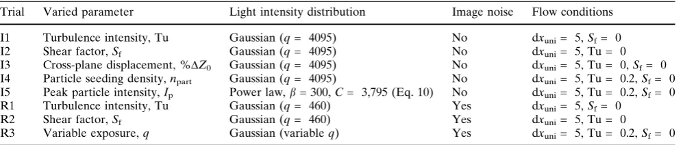
Table 3 Technical specifications for each of the simulated image trials used to evaluate Intensity Capping

Trial Varied parameter Light intensity distribution Image noise Flow conditions

I1 Turbulence intensity, Tu Gaussian (q= 4095) No dxuni= 5,Sf= 0

I2 Shear factor,Sf Gaussian (q= 4095) No dxuni= 5, Tu = 0

I3 Cross-plane displacement, %DZ0 Gaussian (q= 4095) No dxuni= 5, Tu = 0,Sf= 0 I4 Particle seeding density,npart Gaussian (q= 4095) No dxuni= 5, Tu = 0.2,Sf= 0 I5 Peak particle intensity,Ip Power law,b= 300,C= 3,795 (Eq. 10) No dxuni= 5, Tu = 0.2,Sf= 0

R1 Turbulence intensity, Tu Gaussian (q= 460) Yes dxuni= 5,Sf= 0

R2 Shear factor,Sf Gaussian (q= 460) Yes dxuni= 5, Tu = 0

R3 Variable exposure,q Gaussian (variableq) Yes dxuni= 5, Tu = 0.2,Sf= 0

Using simulated images, it is possible to directly compare PIV-derived displacement calculations with the true mean particle displacement. Within each interrogation window, the true mean particle motion was computed as the mean displacement of all particles originating in the window. For each simulated trial, three replicates were performed to smooth variations in results due to the random initial particle location (in all trials) and the random displacement assignments in turbulence trials.

4.3 Results of synthetic image trials

To investigate the mechanisms responsible for the improvements observed with Intensity Capping in

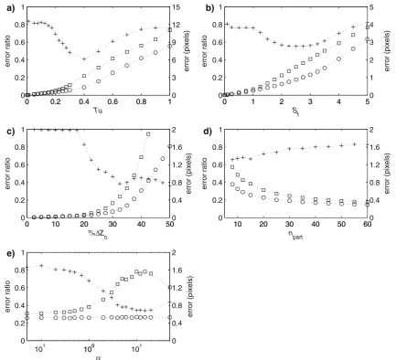
Sect.3, we first consider the ideal simulated images (I1–I5 in Table3; Fig. 7a–e).

Trials I1–I2 investigate the effect of individual par-ticle motion relative to mean parpar-ticle motion via tur-bulence and mean velocity shear. In such flows, the relative motion of bright spots to the mean particle motion may result in PIV errors. Figure 7a and b show that Intensity Capping reduces this displacement error for all values of turbulence intensity, Tu, and shear strength factor, Sf, considered. In turbulent flow,

Intensity Capping yields the greatest improvement (about 60% reduction in rms displacement error from ~3.3 pixels to~1.3 pixels) at around Tu = 0.4 (Fig. 7a). In sheared flow, the greatest improvement (~40% rms error reduction) is observed for levels of shear given by

0 0.2 0.4 0.6 0.8 1

0 0.2 0.4 0.6 0.8

1

error ratio

Tu

0 0.2 0.4 0.6 0.8 10

3 6 9 12 15

error (pixels)

0 1 2 3 4 5

0 0.2 0.4 0.6 0.8

1

error ratio

S

f

0 1 2 3 4 50

1 2 3 4 5

error

(p

ixels

)

10 20 30 40 50 60

0 0.2 0.4 0.6 0.8

1

error ratio

n

part

10 20 30 40 50 600

0.4 0.8

1.2 1.6 2

error

(p

ixels

)

0 10 20 30 40 50

0 0.2 0.4 0.6 0.8

1

error ratio

%∆Z

o

0 10 20 30 40 500

0.4 0.8

1.2 1.6 2

error (pixels)

101 100 101

0 0.2 0.4 0.6 0.8

1

error ratio

α

100

0 0.4 0.8

1.2 1.6 2

error (pixels)

a) b)

c) d)

e)

Fig. 7 Intensity Capping evaluation using ideal simulated images. Squares represent an uncapped rms error (in pixels);

circles represent a capped rms error (in pixels); plus signs

represent the ratio of capped error to uncapped error. Subfigures show the effects of varying:aturbulence intensity,Tu(Trial I1);

Sfin the range~2 to~3 (Fig.7b). Since turbulence and

shear are present in many PIV experiments, Intensity Capping is a very attractive technique for reducing such PIV errors.

Cross-plane particle motion is common to many PIV experiments and may also result in PIV error due to particle pair loss and the generation of bright spots. For example, a particle may become a bright spot as it moves from the edge of the laser light sheet (where illumination is relatively low) to the light sheet center (a region of intense illumination). Particle pair loss may also cause bright spots to correlate with mis-matched particles. Figure7c (Trial I3) shows that Intensity Capping is effective at reducing PIV errors due to cross-plane particle motion, particularly for cross-plane displacements greater than 20% of the laser light sheet thickness.

The relative abundance of bright spots due to vari-ations in particle seeding density also influences the error incurred by PIV. In Trial I4, the particle seeding density, npart, is varied for a constant Tu = 0.2. When

the seeding density is high, a bright spot has a small influence (or degradation potential) on the cross-cor-relation. Figure7d shows that in this case, the un-capped PIV error and benefit of Intensity Capping are both relatively small. When the seeding is low, on the other hand, a bright spot may more readily bias the cross-correlation. In this case, the uncapped PIV error is high and Intensity Capping is particularly effective at reducing this error.

Trial I5 investigates the effectiveness of Intensity Capping for a variable proportion of bright spots in the images. For this trial, the peak particle intensity of each particle is specified by a power law,

IpðkÞ ¼bþC½ðk1Þ=ðN1Þa; ð10Þ

wherekrefers to thekth particle,ais a user-specified exponent, b is the baseline peak particle intensity contribution,Cis the bright spot contribution to peak

0 0.2 0.4 0.6 0.8 1

0 0.2 0.4 0.6 0.8

1

error ratio

Tu

0 0.2 0.4 0.6 0.8 10

3 6 9 12 15

error

(p

ixels

)

0 1 2 3 4 5

0 0.2 0.4 0.6 0.8

1

error ratio

S_f

0 1 2 3 4 50

1 2 3 4 5

error

(p

ixels

)

0 1000 2000 3000 4000

0 0.2 0.4 0.6 0.8

1

error ratio

q

0 1000 2000 3000 40000

0.4 0.8

1.2 1.6 2

error

(p

ixels

)

a)

b)

c)

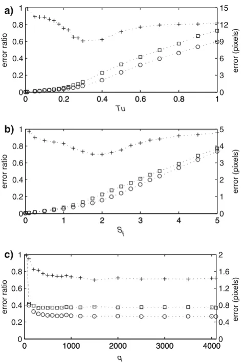
Fig. 8 Intensity Capping evaluation using realistic synthetic images. Squares represent an uncapped rms error (in pixels);

circles represent a capped rms error (in pixels); plus signs

represent the ratio of capped error to uncapped error. Subfigures show the effects of varying:aturbulence intensity,Tu(Trial R1);

bshear factor,Sf(Trial R2); andcmaximum light sheet intensity

q(Trial R3)

101 100 101

0 0.2 0.4 0.6 0.8

1

error ratio

α

Intensity capping CLAHE min/max MHE

0 0.2 0.4 0.6 0.8 1

0 0.2 0.4 0.6 0.8

1

error ratio

Tu

a)

b)

Fig. 9 Comparison of the image-enhancement techniques: Intensity Capping, CLAHE, min/max, and MHE. Subfigures show the effects of varying: a distribution of peak particle intensity,Ip, via the parametera(Trial I5, based on Eq. 10); and

particle intensity, andNis the total number of particles in the image. This model allows the user to control the proportion of bright spots in the image via the expo-nent parameter, a. For a= 0, we recover the top-hat profile (i.e., no variation inIp),Ip= b+ C. Fora= 1,

we have linear variation in Ip across all particles,

ranging frombtob+ C. For largea(a1), we again reduce the variation inIp, such that almost all particles

have Ip = b, while a small number of particles are

allowed to have higher intensities. Figure7e shows that as a increases (and hence more bright particles are generated) for a constant Tu = 0.2, the PIV error in-creases and the improvement gained by Intensity Capping increases. Fora> 20, the uncapped PIV error becomes smaller because the variation in Ip actually

declines, as almost all particles have a uniform peak intensity (Ip= b).

In order to evaluate the performance of Intensity Capping for more realistic image characteristics, three sets of realistic simulated images were analyzed (R1– R3 in Table3). Trials R1–R2 demonstrate the perfor-mance of Intensity Capping for realistic simulated images with variable turbulence intensity and shear. Intensity Capping improves the results for the entire range of turbulence intensities and shear levels, with a peak improvement around Tu~0.3–0.4 and Sf ~ 1.5 –

2.5, respectively (Fig.8a, b).

Trial R3 investigates the effect of variable signal-to-noise ratios by varying the peak particle intensity, q.

Figure 8c reveals that the improvement due to Inten-sity Capping is consistently high when there is a large separation between the peak particle intensity and background noise (q> ~1,000). For peak particle intensities closer to the noise intensity (q< ~1,000), the improvement due to Intensity Capping attenuates, as the capping causes particle intensities to be compara-ble to the background noise.

The simulated images also allow for additional comparison of Intensity Capping with the other image-enhancement techniques: MHE, min/max, and CLAHE. Figure9 shows the error ratio (ratio of rms displacement error for enhanced images to rms dis-placement error for unenhanced images) for Trial I5 and Trial R1.

Figure 9a (Trial I5) investigates the effects of bright spot frequency via the power law intensity model (Eq. 10). The four image-enhancement techniques follow the same general trend, with optimal perfor-mance occurring around 10 < a< 20, a range in which most particles have intensities near the baselineband the remaining particles have elevated (bright) intensi-ties ranging from b to b+ C. For larger a (a > 20), where almost all particles are of the baseline intensityb and few bright spots exist, the benefit of the enhance-ment techniques declines from optimal. The results of Intensity Capping and MHE are almost identical and perform slightly better than the CLAHE and min/max filters.

Figure 9b (Trial R1) investigates the effect of vari-able turbulence levels (the same conditions as shown in Fig.8a). The results indicate that all four image-enhancement techniques reduce the PIV error (error ratio < 1) for typical turbulence levels (Tu < 0.3). The one exception to this observation occurs near Tu = 0 (i.e., Tu = 0.001 and 0.01) where the error in the PIV results from the unenhanced images is very small and thus the error ratio is a poor metric for performance. For very large levels of turbulence (Tu > 0.3), the techniques show a decline in performance. In general, Intensity Capping and MHE demonstrate superior performance for small Tu, while min/max is superior at relatively high Tu.

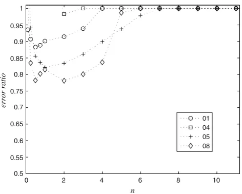
The performance of Intensity Capping was also tested using a set of standard, public domain, synthetic images (Fig.10). Okamoto et al. (2000) produced synthetic PIV images based on three-dimensional LES simulations. For the current study, we analyzed four image pairs from a two-dimensional wall shear flow simulation (http://www.piv.vsj.or.jp/piv/image-e.html): a ‘reference’ image pair (named ‘01’); a ‘dense particle’ image pair (named ‘04’, consisting of 10,000 particles compared to 4,000 particles in the ‘reference’ images);

0 2 4 6 8 10

0.5 0.55 0.6 0.65 0.7 0.75 0.8

0.85 0.9 0.95 1

n

error r

a

tio

01 04 05 08

a ‘sparse particle’ image pair (named ‘05’, consisting of only 1,000 particles); and a ‘large out-of-plane velocity’ image pair (named ‘08’). In all these cases the first two images (out of four provided images) were chosen for the analysis. The images were capped with a range ofn

values and subsequently processed with MatPIV. The results from these standard images are consistent with the analysis of our own synthetic images: the improvement in PIV results due to Intensity Capping increases as the density of particles decreases. Also, Intensity Capping is particularly effective at reducing PIV errors for image pairs with out-of-plane particle motion.

While all of the previous examples demonstrate that Intensity Capping and the existing image-enhancement techniques effectively reduce rms displacement errors, the question remains as to whether these techniques may adversely affect some of the individual vectors (i.e., increase the error). To quantify this degradation effect to individual vectors, we plot histograms of the difference between PIV errors associated with the unenhanced images to those generated by analyzing enhanced images, for all velocity vectors. The differ-ence between the PIV errors is defined such that positive values represent an improvement and negative values represent degradation.

For illustration, histograms are shown for Trial R1, with Tu = 0.2 and background noise present (Fig.11). The percentage of vectors for which the PIV result was improved was 70% for Intensity Capping (Fig.11a)

and 68, 63, and 71% for MHE, min/max, and, CLAHE respectively (Fig. 11b–d). Thus, all of the techniques improve more vectors than they degrade. Additionally, all of the techniques reduce the rms displacement error for this case; the rms displacement errors are reduced from the 0.74 average pixel error associated with the original, unenhanced image (Fig.8a), by 0.25, 0.24, 0.08, and 0.17 pixels for Intensity Capping, MHE, min/max, and CLAHE, respectively. For other trials, similar behavior is typically observed: more than 50% of the vectors are improved and the rms PIV error is reduced.

The source of the degradation of certain individual vectors for Intensity Capping could result from at least two sources: (1) the technique will tend to reduce the separation range between the background noise and the peak particle intensities, and (2) by capping the highest intensities, the correlation peak may broaden (e.g., see Fig. 4). The first effect is minimized by selecting the appropriate level of capping (i.e.,n) such that the particle intensity remains above the back-ground noise and an improvement in the PIV results is observed. To investigate the second effect, we consider the case from Trial I1 when Tu = 0 (i.e., dxvar= 0) and

the images are capped at an extreme value of 1 (i.e., the resulting capped images are binary). Given that there is no background noise and no relative particle motion (dxvar= 0) for this case, the resulting error will

simply result from the ability of the PIV code to find the correlation peak. The rms displacement error was

1 0 1 2 3

0 5 10 15 20

pixels

% of total subwindows

Intensity capping

1 0 1 2 3

0 5 10 15 20

pixels

% of total subwindows

CLAHE

1 0 1 2 3

0 5 10 15 20

pixels

% of total subwindows

min/max

1 0 1 2 3

0 5 10 15 20

pixels

% of total subwindows

MHE

a) b)

c) d)

Fig. 11 Histograms of the displacement error

improvement (pixels) due to image enhancement (positive values represent

improvement and negative values represent

0.008 for the original, uncapped case and 0.010 pixels for the binary, capped case. We conclude that even for this extreme binary capping, where the correlation peak would presumably be broadest, the added error can effectively be neglected (representing only a 0.002 pixel error in a 5 pixel mean displacement).

5 Conclusions

The results of this paper indicate that Intensity Capping offers an efficient solution to the common PIV problem of spurious vectors generated by bright spots that move relative to the mean particle motion. Intensity Capping is implemented prior to PIV analysis and therefore any PIV code, open source or commer-cial, can be used without modification.

In all of the cases considered, Intensity Capping shows excellent performance. For the set of experi-mental images considered, Intensity Capping always yields PIV results with a reduced percentage of spuri-ous vectors, as measured by a local consistency filter. Our analysis shows that a choice ofn= 0.5–3 generally yielded the best results. However, since an optimaln

depends on the particular image noise characteristics, its value should be confirmed for each new set of experiments. For a large set of simulated images, Intensity Capping reduces the rms particle displace-ment error for all parameter ranges considered. Analysis of Intensity Capping in the context of existing image-enhancement techniques shows that it typically performs better or comparably for a wide range of image and flow conditions.

An attractive feature of Intensity Capping is that it has a minor effect on the measurement error. For example, the degradation in pixel displacement accu-racy due to extreme binary capping was found to be negligible. Intensity Capping also only modifies a rel-atively small fraction of the total image pixels relative to other image-enhancement techniques. The image modification only affects those pixels having exceed-ingly high intensities. MHE, min/max, and CLAHE re-map the entire image, including the background noise; background noise may be amplified and may thereby lead to PIV errors. Intensity Capping is different in that it only alters the highest intensity particles (i.e., not the background noise), and thus it avoids noise amplification. Furthermore, the removal of the peak intensity values by Intensity Capping has a minor effect on displacement error since the particle image location information is contained in the intensity gradients that separate the particles from the background. Intensity Capping has less influence on these gradients than

other enhancement techniques relying on spatial filtering. It is also important to note that the pixels affected by Intensity Capping still contribute to the displacement calculation. Bright spots may represent particle pairs that are important to the result of the cross-correlation. Intensity Capping does not eliminate the contribution of these bright pixels, but simply reduces their relative weight and as a result, the cross-correlation better represents the majority of the particle pairs.

It is important to place the proposed Intensity Capping procedure in the context of previous studies of camera bit-depth and PIV image enhancement. Willert (1996) studied the effect of bit-depth on PIV, using scanned photographs. The PIV images were obtained by scanning particle photographs at different depths (1-bit to 8-bit). Willert (1996) found that bit-depth played a minor role in the final measurement uncertainty. For example, PIV results based on binary images consist of only 10–20% more errors than those based on 8-bit images (Willert 1996). This finding and the performance of Intensity Capping indicate that high quality PIV results can be obtained from images of relatively narrow dynamic intensity range. However, it should be noted that Intensity Capping is different from this scanning procedure. In the scanning proce-dure, the intensity values are mapped to a new bit-depth, but bright spots remain. Intensity Capping, on the other hand, removes bright spots without changing the bit-depth.

Capping makes it a particularly attractive technique for large PIV data sets.

Finally, the proposed Intensity Capping technique could be further developed. Non-uniform (tile by tile) intensity capping may be more effective when large spatial variations in the image background exist. To achieve optimal results, it may then be necessary to perform intensity capping within discrete tiles using local, rather than global, intensity statistics. Intensity capping could also be developed into an error detec-tion tool. The user could analyze an image pair with and without Intensity Capping. The results from Intensity Capping may then be used as a filter to reject spurious vectors in the PIV results from the uncapped images. This may be particularly useful when a user wishes to process unenhanced images, but still seeks to validate and filter the results.

Acknowledgments The authors are grateful for the discussions with J. Rosman, J. Koseff, and S. Monismith and the technical help provided by R. Gurka and R. Rosenzweig. The authors extend special thanks to M. Wernet for implementing his SPOF technique. The authors would like to acknowledge contributions to the Ocean PIV project by J. Jaffe, P. Roberts, F. Simonet, P. Franks, S. Monismith, C. Troy, and A. Horner-Devine. Support for Ocean PIV was provided by NSF grant OCE-0220213. R. Lowe acknowledges support from NSF grant OCE-0453117.

References

Cowen EA, Monismith SG (1997) A hybrid digital particle tracking velocimetry technique. Exp Fluids 22:199–211 Dellenback PA, Macharivilakathu J, Pierce SR (2000)

Contrast-enhancement techniques for particle-image velocimetry. Appl Optics 39(32):5978–5990

Fore LB, Tung AT, Buchanan JR, Welch JW (2005) Nonlinear temporal filtering of time-resolved digital particle image velocimetry data. Exp Fluids 39:22–31

Gurka R (1999) Dynamics of a flexible tube in the turbulent gas flow of a twin fluid atomizer. M.Sc. thesis, Technion, Israel Gurka R, Liberzon A, Hefetz D, Rubinstein D, Shavit U (1999) Computation of Pressure Distribution Using PIV Velocity Data. In: Third international workshop on particle image velocimetry, Santa Barbara, California, pp. 671–6, Septem-ber 16–18, 1999

Keane RD, Adrian RJ (1992) Theory of cross-correlation analysis of PIV images. Appl Sci Res 49:191–215

Lowe RJ (2005) The effect of surface waves on mass and momentum transfer processes in shallow coral reef systems. PhD thesis, Stanford University

Okamoto K, Nishio S, Saga T, Kobayashi T (2000) Standard images for particle-image velocimetry. Meas Sci Technol 11:685–691

Raffel M, Willert C, Kompenhans J (1998) Particle image velocimetry: a practical guide. Springer, Berlin Heidelberg New York

Rosenzweig R (2005) The macroscopic velocity profile near permeable interfaces: piv measurements, numerical simula-tions, and an analytical solution of the laminar problem. M.Sc. thesis, Technion, Israel

Roth GI, Katz J (2001) Five techniques for increasing the speed and accuracy of PIV interrogation. Meas Sci Technol 12:238–245

Shavit U, Moltchanov S, Agnon Y (2003) Particles resuspension in waves using visualization and PIV measurements—coher-ence and intermittency. Int J Multiph Flow 29:1183–1192 Sveen KJ (2004) An introduction to MatPIV v. 1.6.1, eprint series,

Dept. of Math. University of Oslo, ‘‘Mechanics and Applied Mathematics‘‘, NO. 2 ISSN 0809–4403, August, 2004 Wernet MP (2005) Symmetric phase only filtering: a new paradigm

for DPIV Data Processing. Meas Sci Technol 16:601–618 Westerweel J (1993) Digital Particle Image Velocimetry. Theory

and Practice, PhD Thesis, Delft University of Technology, The Netherlands