www.ann-geophys.net/27/3949/2009/
© Author(s) 2009. This work is distributed under the Creative Commons Attribution 3.0 License.
Annales
Geophysicae
On the error estimation of multi-spacecraft timing method
X.-Z. Zhou1,2, Z. Y. Pu2, Q.-G. Zong2,3, P. Song3, S. Y. Fu2, J. Wang2, and H. Zhang1
1Institute of Geophysics and Planetary Physics, University of California, Los Angeles, CA, USA 2Institute of Space Physics and Applied Technology, Peking University, Beijing, China
3Center for Atmospheric Research, University of Massachusetts, Lowell, MA, USA
Received: 27 June 2009 – Revised: 13 October 2009 – Accepted: 14 October 2009 – Published: 20 October 2009
Abstract. The multi-spacecraft timing method, a data anal-ysis technique based on four-point measurements to obtain the normal vector and velocity of an observed boundary, has been widely applied to various discontinuities in the solar wind and the magnetosphere studies. In this paper, we per-form simulations to analyze the errors of the timing method by specifying the error sources to the uncertainties in the de-termination of the time delays between each spacecraft pair. It is shown that the timing method may have large errors if either the spacecraft tetrahedron is largely elongated and/or flattened, or the discontinuity moves much slower than the constellation itself. The results, therefore, suggest that some of the applications of the timing method require reexami-nation with special caution, in particular for the studies of the slow-moving discontinuities associated with, for exam-ple, the plasmaspheric plumes.
Keywords. Interplanetary physics (Instruments and tech-niques) – Magnetospheric physics (Plasmasphere; Instru-ments and techniques)
1 Introduction
Multi-spacecraft missions, such as the Cluster (Escoubet et al., 1997), THEMIS (Angelopoulos, 2008), and the fu-ture MMS mission, were designed with the potential to un-ambiguously separate the spatial and temporal variabilities. Since the idea of the Cluster mission with four identical satel-lites making simultaneous measurements at different loca-tions was proposed in the 1980s, many data analysis tech-niques have been developed, based on time series of four-point observations, to enable the three-dimensional exami-nation of the observed structures in space plasma. Among these techniques, the one most widely used is probably the
Correspondence to: X.-Z. Zhou
multi-spacecraft timing method, sometimes referred to as the triangulation method and/or the time-delay method, in the studies of the orientation and motion of planar discontinuities (Russell et al., 1983; Harvey, 1998; Sonnerup et al., 2008).
Assuming that a one-dimensional discontinuity moves with a constant velocity (which registers a pure spatial vari-ation as a set of time-series varivari-ations), the multi-spacecraft timing method (hereinafter referred to as the timing method) makes use of the measured time differences between the pas-sage of the discontinuity over satellites, along with the rel-ative positions between the crossing locations, to calculate the normal unit vector N and the normal velocity V. Tak-ing the four-spacecraft Cluster mission as the example, if the discontinuity can be identified unambiguously, i.e., all of the discontinuity passage times tαare well determined, we have:
Rα1·N=V(tα−t1), 2≤α≤4 (1)
where spacecraft 1 is arbitrarily taken as the reference, and
Rα1represents the relative position between the discontinuity
crossing locations observed by spacecraftαand spacecraft 1. As long as the four satellites are not coplanar, the equation yields a unique solution of the normal vector and the normal velocity.
It should be kept in mind that the position vectors of dif-ferent satellites are not simultaneous as the crossings occur at different times. Therefore, the instantaneous interspace-craft distances Dα1, which can be directly obtained (from
the European Space Operations Centre for the Cluster mis-sion), cannot simply be used to replace the relative position vectors Rα1 in Eq. (1). Instead, the position changes of the
spacecraft during these time intervals have to be taken into account, with the terms of(tα−t1)VCbeing added to Dα1to
obtain the corresponding Rα1 vectors, where VC represents the velocity of the Cluster constellation.
one-dimensional structure, or the discontinuity itself may evolve in time. One way to improve the results is to deter-mine the optimal relative time delay for each spacecraft pair, which can be calculated either by maximizing the value of the cross-correlation (e.g., Song and Russell, 1999) between these data streams, or by the application of the Local Wavelet Correlation (LWC) technique (Soucek et al., 2004). A total of six time delays tαβ(1<α≤4,1≤β<α) can be calculated, and the six corresponding relative position vectors Rαβ are also obtained, by adding the tαβVC term to the interspace-craft distances Dαβ. Thus we can obtain an over-determined equation set containing three unknowns and six independent equations. By minimizing the function
S= 4
X
α=1
α−1
X
β=1
[N·Rαβ−Vtαβ]2
= 4
X
α=1
α−1
X
β=1
[N·Dαβ−(V−N·VC)tαβ]2 (2)
a least-squares approach can be used to determine the opti-mal solution, i.e., the noropti-mal vector and the noropti-mal velocity of the observed discontinuity (Harvey, 1998).
Equation (2) further highlights the different roles Rαβand
Dαβplay in the application of the timing method, namely, if one select the instantaneous interspacecraft distances Dαβ in-stead of using the relative position vectors Rαβin the timing method, the resulting velocity would be in the frame moving with the Cluster constellation. As we know that in most cases the velocity of the discontinuity should be cast in the Earth’s frame for physical significance and usefulness, it is important to make sure that the relative position vectors Rαβ are used (instead of Dαβ) when performing the timing analysis.
Since the launch of the Cluster constellation, the timing method has been applied to various types of discontinuities in the near-Earth space, e.g., the interplanetary discontinu-ities (Knetter et al., 2003, 2004), the terrestrial bow shock (Bale et al., 2003; Maksimovic et al., 2003), the magne-topause (Haaland et al., 2004; Owen et al., 2004), the plasma sheet (Dewhurst et al., 2004; Runov et al., 2005), the cusp re-gion (Taylor et al., 2004; Zong et al., 2004), and the plasma-pause/plume (Darrouzet et al., 2004, 2006). The timing method has also been modified (Zhou et al., 2006a; Zhou et al., 2006b) to determine the orientations and the veloci-ties of 2-D structures, such as flux ropes. Furthermore, it should be noted that there are modified versions of the tim-ing method to consider the acceleration term and/or the cur-vature term (Chanteur, 1998; Dunlop et al., 2002; Haaland et al., 2004), although in this paper, we will focus only on the classical version (with a planar discontinuity moving at a constant speed) of the method described above.
In order to avoid the improper usage of the timing method, the estimation of the errors both in the normal direction and in the velocity becomes very important. However, only a few attempts have been made on this issue (Chanteur, 1998;
Cornilleau-Wehrlin et al., 2003; Vogt et al., 2008). One of the most extensive studies was made by Knetter (2005), who applied the timing method on fast solar wind discontinuities and analyzed the parameters affecting the error of the timing method. As was noted in their works, the detected instanta-neous satellite distances Dαβ contain very minor uncertain-ties, and the error of the timing method mostly arises from the uncertainties in the determination of the six time delays
tαβ.
In this paper, we examine the error introduced in the time delay determination, which is assumed to be normally dis-tributed with zero mean and a standard deviation of 1 s (in comparison with the typical time-resolution of 4 s which is the Cluster spin period). This random error, being treated as the only error source, is embedded in the performance of the timing method on a set of simulated Cluster crossings over a discontinuity moving at a constant velocity, to compare the resulting normal directions and velocities with the modeled ones. We find that the error depends not only on the shape of the Cluster tetrahedron, but also on the speed of the dis-continuity compared with that of the Cluster constellation. For those cases in which the discontinuity moves at a lower speed, the error would be significantly enlarged, which re-quires the application of timing method with special caution, to the slow-moving discontinuities such as the plasmaspheric plumes.
2 Accuracy of the timing method
For the Cluster mission, the tetrahedron composed by the four spacecraft has the configurations varying continuously along its orbit around the Earth. Typically, the tetrahedron appears to be fairly regular at the apogee of the Cluster constellation, but it is significantly stretched at the perigee, which can be also seen in Fig. 16.1 of Robert et al. (1998a).
The best way to describe the geometry of the Cluster tetra-hedron is to use a 2-D geometric factor, as the combination of the elongation parameter E and the planarity parameter P (Robert et al., 1998b). Both of the parameters are derived from the eigenvalues of the tetrahedron volumetric tensor, which can be also determined by the six interspacecraft dis-tance vectors Dαβ(for more detail, see Robert et al. (1998b) and Harvey (1998)). The values of E and P vary from 0 to 1: for a regular tetrahedron, E and P are both zero; if the tetra-hedron is stretched, the value of E will increase, until E=1 when the satellites are on a straight line; if the tetrahedron is squashed, the value of P will increase, and the satellites will lie in a plane if P equals 1.
(1998b) are applied to ensure that the E and P values of these tetrahedra cover the whole E-P plane homogeneously.
As the second step, we simulate a planar discontinuity moving along its normal direction (the−x-direction) with the speed of 50 km/s, and we have all of the tetrahedra moving in the +x-direction, with a relatively smaller speed of 5 km/s. The time delays between each spacecraft pair when they ob-serve the discontinuity, along with their relative position vec-tors, can thus be unambiguously determined. Here we further normalize the size of each modeled tetrahedron to have the averaged absolute value of the six corresponding time delays equal to 30 s, which is the typical value and of practical inter-est in the timing method application to the real Cluster data: in those cases with much longer time delays, any real discon-tinuities would evolve significantly which might invalidate the timing method, while those cases with much shorter de-lays would suffer from the quantization effects owing to the limited time resolution of the data (typically 4 s which is the spin period of the Cluster satellites).
As we discussed before, there are further error sources in the determination of the six time delays, e.g., the non-planar properties of the discontinuity as well as the super-posed structures and/or fluctuations. In fact, the classical way to obtain the time delays requires a process of maximizing the cross-correlation function, and the uncertainties in the re-sulting time delays, according to Eq. (1.7) of Sonnerup et al. (2008), depend on several factors: the number of data points, the obtained maximum correlation coefficient, the average slope square of the signal, and the average magnitude square of the signal deviation from its average value. Furthermore, the cross-correlation process is somewhat arbitrary: the data window selection and the interpolation method selection may both produce errors (Song and Russell, 1999). To reduce these errors, a more sophisticated technique, called the Lo-cal Wavelet Correlation (Soucek et al., 2004), was also pre-sented. However, as was admitted by Soucek et al. (2004), the error cannot be fully eliminated unless the signals are identical up to a shift in time.
Here, as an example, we assume a normally distributed random error with zero mean and a standard deviation of 1 s, for each spacecraft pair, to adjust the six “theoretical” time delays. As the interspacecraft distance vectors Dαβ remain unchanged, the relative position vectors Rαβ between each two satellites can be accordingly adjusted based on the result-ing time delays and the modeled Dαβvalues, which is impor-tant as the uncertainties in the determination of the time delay would also produce uncertainties in the relative positions of the corresponding spacecraft pair. The timing analysis can thus be performed through Eq. (2) to calculate the normal di-rection and the normal velocity of the certain discontinuity.
The last step is to compare the results obtained by the timing method with the modeled ones (50 km/s in the− x-direction), to estimate the reliability of the timing method. For each of the 1600 tetrahedra, the second step is performed 1000 times with the time delays adjusted with random errors,
and the averaged relative error of the normal velocity com-ponent can be expressed as
ε= 1 N
N X
n=1
[(VT −VM) 2
VM2
]1/2, N =1000 (3)
where VT and VM represent the calculated normal compo-nent of the velocity and the modeled one (50 km/s), respec-tively.
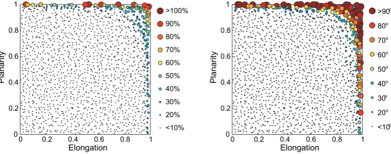
The relation between the relative error of the normal veloc-ity and the tetrahedron geometry is shown in the left panel of Fig. 1. The sizes and the colors of the circles indicate the values of the relative errors: for those cases with the error less than 10%, the circles are very small, while the largest circles correspond to a relative error of greater than 100%. Note that the circles are sorted by size before being plotted, so there are no small circles hidden behind larger ones.
The uncertainty in the determination of the normal direc-tion, on the other hand, is shown in the right panel of Fig. 1. The uncertainty is inferred by the 90-percent confidence in-terval (CI) of the angle between the calculated normal direc-tion and the modeled one (along the−x-axis). The small-est circles correspond to the CIs of less than 10◦, which means that we are 90% confident that the angular error is less than 10◦, while the largest ones suggest the uncertainties of greater than 90◦.
It is clear that the errors are generally small except for the cases when the four spacecraft lie approximately along a straight line or within a plane. In these two extreme cases, the component equations in Eq. (1) degenerate to one and two component equations, respectively, leaving some unknowns undetermined. The result, therefore, is not surprising: for the cases of E close to 1, the separation vectors between each pair of satellites are in very similar directions, and therefore can hardly provide the information in the perpendicular di-rections; for the cases of high P, the separation vectors are generally coplanar, and the speed normal to the plane cannot be determined.
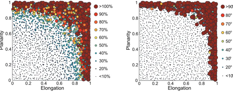
Note that here we use the discontinuity speed of 50 km/s which is ten times greater than the speed of the Cluster constellation (5 km/s). However, if the discontinuity moves much slower, say, 0.5 km/s (still in the−x-direction), the un-certainties of the timing method can be calculated to be quite different, as shown in Fig. 2.
The relative errors on the normal velocities shown in the left panel of Fig. 2, although not solely dependent on the val-ues of E and P because of the differences in the orientations of these tetrahedra, are always greater than 20% even in the cases of regular tetrahedra. For E or P values greater than 0.8, the errors are generally greater than 100%, and even as large as 1000% for E or P close to 1. Similarly, the uncer-tainties in the normal directions (right panel of Fig. 2) are also much greater than those in the previous case.
0 0.2 0.4 0.6 0.8 1 0
0.2 0.4 0.6 0.8 1
Elongation
Planarity
<10o 20o 30o 40o 50o 60o 70o 80o >90o
0 0.2 0.4 0.6 0.8 1
Planarity
<10% 20% 30% 40% 50% 60% 70% 80% 90% >100%
0 0.2 0.4 0.6 0.8 1
Elongation
Fig. 1. Influence of the tetrahedron configuration, parameter P and E, on the error of the timing method, denoted by the size and color of the circles, when the modeled discontinuity moves ten times faster than the Cluster constellation. Left and right panels correspond to the relative error in the determination of the normal velocity component and the 90-percent confidence interval of the angle between the normal direction and the modeled one, respectively.
0 0.2 0.4 0.6 0.8 1
0 0.2 0.4 0.6 0.8 1
Planarity
<10% 20% 30% 40% 50% 60% 70% 80% 90% >100%
Elongation
0 0.2 0.4 0.6 0.8 1
Planarity
0 0.2 0.4 0.6 0.8 1
Elongation
<10o
20o
30o
40o
50o
60o
70o
80o
[image:4.595.102.495.63.218.2]>90o
Fig. 2. Same format as in Fig. 1, but the modeled discontinuity speed is 1/10 of the Cluster speed.
transformation process between two reference systems. If we are in the frame moving along with the Cluster constellation, as was suggested before, the relative position vectors Rαβ in Eq. (2) could be replaced by the interspacecraft distance vectors Dαβ. Therefore, if the previous two test runs are per-formed in the Cluster’s frame, it is not necessary to adjust the
Dαβvalues to obtain Rαβ, and the latter run differs from the former one by having a discontinuity velocity of 5.5 km/s ten times smaller than that in the former run. Note that the Dαβ values in the latter run are also ten times smaller, which is produced in the normalization process to have the averaged absolute value of the six time delays equal to 30 s.
The factors of ten, however, can be eliminated by substi-tuting the V and Dαβ values to Eq. (2), which suggests the relative errors ε0 in the determination of the discontinuity
velocity be the same for the two test runs if both performed in the Cluster’s frame. As we know that the transformation
to another frame of reference would not change the value of the absolute error, we have
ε1|VD1| =ε0|VD0| =ε0|VD1−VC1| (4)
where VD0, VD1, and VC1 represent the discontinuity
ve-locity in the frame moving with the Cluster constellation, the discontinuity velocity in the Earth’s frame of reference, and the Cluster velocity in the Earth’s frame, respectively. Therefore, if the discontinuity moves much slower than the Cluster constellation in the Earth’s frame, the satisfaction of Eq. (4) results in significant amplification of the relative error
ε1in the Earth’s frame. In other words, since the velocity of
[image:4.595.102.497.300.454.2]V = 0.57 km/sn
AIN
V = 0.77 km/sn
N x 1e
PPIN
V = 0.14 km/sn
AOUT
V = 0.33 km/sn
V = 0.42 km/sn
N x 10e
PPOUT
[image:5.595.102.498.61.268.2]Z
Fig. 3. The plasmapause/plume crossings of the Cluster constellation, adapted from Darrouzet et al. (2004). The densities for an inbound and an outbound are shown with a factor-of-10 shift in the upper traces. The labeled speeds of the moving structures were derived from the timing method.
The error amplification effect, therefore, suggests that the uncertainties of the timing method may be large not only in the cases when the Cluster tetrahedron is greatly elongated or flattened, but also when the discontinuity moves much more slowly than the Cluster constellation. One example of the appearance of possible greater uncertainties occurs when the Cluster satellites move relatively faster with elongated con-figurations near their perigees and encounter slow moving plasmaspheric structures, and the applications of the timing method under these conditions should be carried out with special caution.
3 Example of applications
On 11 April 2002, between 04:15 and 06:30 UT, the Cluster satellites experienced a plasmasphere crossing and observed a plasmaspheric plume outside the plasmasphere (Darrouzet et al., 2004). Darrouzet et al. used the EFW (Gustafsson et al., 1997) and WHISPER (D´ecr´eau et al., 1997) measure-ments to obtain the electron densities and applied the timing method to determining the normal velocity of the plume.
However, it can be clearly seen in Fig. 3 that there are fluc-tuations superposed on the discontinuity, and the time differ-ences between the observations of different satellites contin-uously evolve in time, especially during the Cluster inbound pass. Therefore, it might be relatively hard to determine the time delays accurately.
The small error in the determination of the time delays, on the other hand, can be significantly enlarged in the ap-plication of the timing method. As is shown in Fig. 3, the estimated velocity of the discontinuity is typically one order
smaller than that of the Cluster constellation (4.6 km/s), and the averaged absolute value of the time delays between each spacecraft pair is around 30 s (see Fig. 5 of Darrouzet et al., 2004). Therefore, Fig. 2 can be used to estimate the error in the application of the timing method. During this time period, the Cluster tetrahedron elongation parameter E was 0.8, and the planarity parameter P was 0.2, which suggests that the uncertainties in the velocity determination could be as large as 100%, as the direction determination might be more reliable.
The uncertainty levels of∼100%, therefore, suggest that one should avoid directly comparing two resulting velocities during different time intervals, although it is safe to claim that the plume moves very slowly. In other words, it is quite possible that some of the conclusions drawn by Darrouzet et al. (2004), e.g., the velocities measured along the inbound pass being larger than those along the outbound pass, are within the error bar of the data analysis if the obtained time delays have the uncertainties of∼1 s or more. Therefore, it may be necessary to carefully reexamine the case, for exam-ple, by using the Eq. (1.7) of Sonnerup et al. (2008), to make sure that all of the time delays are accurately determined with the errors much smaller than 1 s despite the effect of the ir-regularities and the fluctuations shown in Fig. 3.
Besides estimating the time delay errors based on Eq. (1.7) of Sonnerup et al. (2008), another way to assess the reliability of the timing method is to calculate all of the four time delay residuals
0 0.2 0.4 0.6 0.8 1 0
0.2 0.4 0.6 0.8 1
Planarity
<10% 20% 30% 40% 50% 60% 70% 80% 90% >100%
Elongation 0 0.2 0.4 0.6 0.8 1
0 0.2 0.4 0.6 0.8 1
Planarity
Elongation
<10o
20o
30o
40o
50o
60o
70o
80o
[image:6.595.101.494.63.218.2]>90o
Fig. 4. Same format as in Fig. 2, but only those cases with all of the four residuals smaller than 1 s are selected in the simulation.
to higher reliabilities of the timing method. Here we perform the same simulation steps, again with the modeled discon-tinuity moving at 0.5 km/s in the−x-direction and the time delay standard deviation of 1 s, but select only those cases with all of the four residuals smaller than 1 s, to calculate the uncertainties of the timing method. The results are shown in Fig. 4, which may be directly compared with the uncertain-ties shown in Fig. 2.
It is shown that the uncertainties in Fig. 4 are reduced, es-pecially those in the velocity determination. Given the E and
P values of 0.8 and 0.2, respectively, the uncertainties in the
velocity determination would be∼30−40%, which are much smaller than the∼100% ones suggested in Fig. 2. In other words, to ensure the appropriate usage of the timing method in this particular Darrouzet et al. (2004) event, one has to make sure that either the time delays are accurately deter-mined (with uncertainties much smaller than 1 s), or all of the time delay residuals are adequately small (less than 1 s). Without these reexaminations, as we suggested before, some of the Darrouzet et al. (2004) conclusions, e.g., the plume ve-locities during the inbound pass being larger than those along the outbound pass, may be less convincing as they are likely to be within the error bar of the timing method.
4 Summary
In this study, we have performed simulations to estimate the uncertainty of the multi-spacecraft timing method, to inves-tigate its dependence on the configuration of the spacecraft tetrahedron and the speed of the observed discontinuity in comparison with the constellation speed. By limiting the er-ror sources of the timing method to the random erer-rors pro-duced in the determination of the time delays between each spacecraft pair, we have found that the uncertainty of the timing method could be very significant if the tetrahedron is largely elongated or flattened. Furthermore, if the dis-continuity moves much more slowly than the constellation,
a small error in the determination of the speed in the satellite frame of reference can be translated to a large relative error. The error estimation, therefore, provides a way for the users of the timing method to evaluate their result based on the es-timated uncertainty levels in the determination of the time delays. For instance, in the study of slow-moving disconti-nuities, such as the plasmaspheric plumes (Darrouzet et al., 2004), even a minor error in the determination of the time delays may result in huge errors, a result that suggests that the timing method should be used with caution and the pre-dictions from an analysis should be made with due attention to the uncertainties in the method.
Acknowledgements. The authors thank V. Angelopoulos at UCLA
for helpful discussions and suggestions. We would like to acknowl-edge NASA (grant NAS5-02099) for the support of our work at UCLA, and the work at Peking University was supported by NSFC grants 40390152, 40425004 and 40528005.
Topical Editor I. A. Daglis thanks two anonymous referees for their help in evaluating this paper.
References
Angelopoulos, V.: The THEMIS Mission, Space Sci. Rev., 141, 5– 34, doi:10.1007/s11214-008-9336-1, 2008.
Bale, S. D., Mozer, F. S., and Horbury, T. S.: Density-Transition Scale at Quasiperpendicular Collisionless Shocks, Phys. Rev. Lett., 91, 265004, doi:10.1103/PhysRevLett.91.265004, 2003. Chanteur, G.: Spatial interpolation for four spacecraft: Theory,
in: Analysis Methods for Multi Spacecraft Data, edited by: Paschmann, G. and Daly, P. W., p. 349, ESA, Bern, Switzerland, 1998.
Darrouzet, F., D´ecr´eau, P. M. E., De Keyser, J., Masson, A., Gal-lagher, D. L., Santolik, O., Sandel, B. R., Trotignon, J. G., Rauch, J. L., Le Guirriec, E., Canu, P., Sedgemore, F., Andr´e, M., and Lemaire, J. F.: Density structures inside the plasmasphere: Clus-ter observations, Ann. Geophys., 22, 2577–2585, 2004, http://www.ann-geophys.net/22/2577/2004/.
Darrouzet, F., De Keyser, J., D´ecr´eau, P. M. E., Gallagher, D. L., Pierrard, V., Lemaire, J. F., Sandel, B. R., Dandouras, I., Matsui, H., Dunlop, M., Cabrera, J., Masson, A., Canu, P., Trotignon, J. G., Rauch, J. L., and Andr´e, M.: Analysis of plasmaspheric plumes: CLUSTER and IMAGE observations, Ann. Geophys., 24, 1737–1758, 2006,
http://www.ann-geophys.net/24/1737/2006/.
D´ecr´eau, P. M. E., Fergeau, P., Krannosels’kikh, V., Leveque, M., Martin, P., Randriamboarison, O., Sene, F. X., Trotignon, J. G., Canu, P., and Mogensen, P. B.: Whisper, a Resonance Sounder and Wave Analyser: Performances and Perspectives for the Clus-ter Mission, Space Sci. Rev., 79, 157–193, 1997.
Dewhurst, J. P., Owen, C. J., Fazakerley, A. N., and Balogh, A.: Thinning and expansion of the substorm plasma sheet: Cluster PEACE timing analysis, Ann. Geophys., 22, 4165–4184, 2004, http://www.ann-geophys.net/22/4165/2004/.
Dunlop, M. W., Balogh, A., and Glassmeier, K.-H.: Four-point Cluster application of magnetic field analysis tools: The dis-continuity analyzer, J. Geophys. Res., 107, 1385, doi:10.1029/ 2001JA005089, 2002.
Escoubet, C. P., Schmidt, R., and Goldstein, M. L.: Cluster - Sci-ence and Mission Overview, Space Sci. Rev., 79, 11–32, 1997. Gustafsson, G., Bostrom, R., Holback, B., Holmgren, G., Lundgren,
A., Stasiewicz, K., Ahlen, L., Mozer, F. S., Pankow, D., Harvey, P., Berg, P., Ulrich, R., Pedersen, A., Schmidt, R., Butler, A., Fransen, A. W. C., Klinge, D., Thomsen, M., Falthammar, C.-G., Lindqvist, P.-A., Christenson, S., Holtet, J., Lybekk, B., Sten, T. A., Tanskanen, P., Lappalainen, K., and Wygant, J.: The Elec-tric Field and Wave Experiment for the Cluster Mission, Space Sci. Rev., 79, 137–156, 1997.
Haaland, S. E., Sonnerup, B. U. ¨O., Dunlop, M. W., Balogh, A., Georgescu, E., Hasegawa, H., Klecker, B., Paschmann, G., Puhl-Quinn, P., R`eme, H., Vaith, H., and Vaivads, A.: Four-spacecraft determination of magnetopause orientation, motion and thick-ness: comparison with results from single-spacecraft methods, Ann. Geophys., 22, 1347–1365, 2004,
http://www.ann-geophys.net/22/1347/2004/.
Harvey, C. C.: Spatial Gradients and the Volumetric Tensor, in: Analysis Methods for Multi-spacecraft Data, edited by: Paschmann, G. and Daly, P., pp. 307–322, ISSI/ESA, Nether-lands, 1998.
Knetter, T.: A new Perspective of the Solar Wind Micro-Structure due to Multi-Point Observations of Discontinuities, PhD Thesis, Universit¨at zu K¨oln, Germany, 2005.
Knetter, T., Neubauer, F. M., Horbury, T., and Balogh, A.: Discon-tinuity observations with cluster, Adv. Space Res., 32, 543–548, doi:10.1016/S0273-1177(03)00335-1, 2003.
Knetter, T., Neubauer, F. M., Horbury, T., and Balogh, A.: Four-point discontinuity observations using Cluster magnetic field data: A statistical survey, J. Geophys. Res., 109, 6102, doi: 10.1029/2003JA010099, 2004.
Maksimovic, M., Bale, S. D., Horbury, T. S., and Andr´e, M.: Bow shock motions observed with CLUSTER, Geophys. Res. Lett.,
30, 070000–1, doi:10.1029/2002GL016761, 2003.
Owen, C. J., Taylor, M. G. G. T., Krauklis, I. C., Fazakerley, A. N., Dunlop, M. W., and Bosqued, J. M.: Cluster observations of surface waves on the dawn flank magnetopause, Ann. Geophys., 22, 971–983, 2004, http://www.ann-geophys.net/22/971/2004/. Robert, P., Dunlop, M. W., Roux, A., and Chanteur, G.: Accuracy
of Current Determination, in: Analysis Methods for Multi Space-craft Data, edited by: Paschmann, G. and Daly, P. W., pp. 395– 418, ESA, Bern, Switzerland, 1998a.
Robert, P., Roux, A., Harvey, C. C., Dunlop, M. W., Daly, W. P., and Glassmeier, K.-H.: Tetrahedron Geometric Factors, in: Analysis Methods for Multi Spacecraft Data, edited by: Paschmann, G. and Daly, P. W., pp. 323–348, ESA, Bern, Switzerland, 1998b. Runov, A., Sergeev, V. A., Baumjohann, W., Nakamura, R.,
Ap-atenkov, S., Asano, Y., Volwerk, M., V¨or¨os, Z., Zhang, T. L., Petrukovich, A., Balogh, A., Sauvaud, J.-A., Klecker, B., and R`eme, H.: Electric current and magnetic field geometry in flap-ping magnetotail current sheets, Ann. Geophys., 23, 1391–1403, 2005, http://www.ann-geophys.net/23/1391/2005/.
Russell, C. T., Mellott, M. M., Smith, E. J., and King, J. H.: Mul-tiple Spacecraft Observations of Interplanetary Shocks: Four Spacecraft Determination of Shock Normals, J. Geophys. Res., 88, 4739–4748, 1983.
Song, P. and Russell, C. T.: Time Series Data Analyses in Space Physics, Space Sci. Rev., 87, 387–463, doi:10.1023/A: 1005035800454, 1999.
Sonnerup, B. U. O., Haaland, S. E., and Paschmann, G.: Disconti-nuity Orientation, Motion, and Thickness, in: Multi-Spacecraft Analysis Methods Revisited, edited by: Paschmann, G. and Daly, P., pp. 1–15, ISSI/ESA, Netherlands, 2008.
Soucek, J., Dudok de Wit, T., Dunlop, M., and D´ecr´eau, P.: Lo-cal wavelet correlation: applicationto timing analysis of multi-satellite CLUSTER data, Ann. Geophys., 22, 4185–4196, 2004, http://www.ann-geophys.net/22/4185/2004/.
Taylor, M. G. G. T., Dunlop, M. W., Lavraud, B., Vontrat-Reberac, A., Owen, C. J., D´ecr´eau, P., Tr´avncek, P., Elphic, R. C., Friedel, R. H. W., Dewhurst, J. P., Wang, Y., Fazakerley, A., Balogh, A., R`eme, H., and Daly, P. W.: Cluster observations of a com-plex high-altitude cusp passage during highly variable IMF, Ann. Geophys., 22, 3707–3719, 2004,
http://www.ann-geophys.net/22/3707/2004/.
Vogt, J., Paschmann, G., and Chanteur, G.: Reciprocal Vectors, in: Multi-Spacecraft Analysis Methods Revisited, edited by: Paschmann, G. and Daly, P., pp. 33–46, ISSI/ESA, Netherlands, 2008.
Zhou, X.-Z., Zong, Q.-G., Pu, Z. Y., Fritz, T. A., Dunlop, M. W., Shi, Q. Q., Wang, J., and Wei, Y.: Multiple Triangulation Anal-ysis: another approach to determine the orientation of magnetic flux ropes, Ann. Geophys., 24, 1759–1765, 2006a,
http://www.ann-geophys.net/24/1759/2006/.