DERIVATIVES
GRAEME WEST AND LYDIA WEST, FINANCIAL MODELLING AGENCY©
Contents
1. Introduction 2
2. European Bond Options 2
2.1. Different volatility measures 3
3. Caplets and Floorlets 3
4. Caps and Floors 4
4.1. A call/put on rates is a put/call on a bond 4
4.2. Greeks 5
5. Stripping Black caps into caplets 7
6. Swaptions 10
6.1. Valuation 11
6.2. Greeks 12
7. Why Black is useless for exotics 13
8. Exercises 13
Date: July 11, 2011.
Bibliography 15
1. Introduction
We consider the Black Model for futures/forwards which is the market standard for quoting prices (via implied volatilities). Black [1976] considered the problem of writing options on commodity futures and this was the first “natural” extension of the Black-Scholes model. This model also is used to price options on interest rates and interest rate sensitive instruments such as bonds. Since the Black-Scholes analysis assumes constant (or deterministic) interest rates, and so forward interest rates are realised, it is difficult initially to see how this model applies to interest rate dependent derivatives.
However, iff is a forward interest rate, it can be shown that it is consistent to assume that
• The discounting process can be taken to be the existing yield curve. • The forward rates are stochastic and log-normally distributed.
The forward rates will be log-normally distributed in what is called theT-forward measure, where T is the pay date of the option. This model is consistent is within the domain of the LIBOR market model. We can proceed to use Black’s model without knowing any of the theory of the LMM; however, Black’s model cannot safely be used to value more complicated products where the payoff depends on observations at multiple dates.
2. European Bond Options
The clean (quoted) price for a bond is related to the all-in (dirty, cash) price via:
A=C+IA(t) (1)
where the accrued interestIA(t) is the accrued interest as of datet, and is non-zero between coupon dates. The forward price is a carried all-in price, not a clean price. The option strike priceKmight be a clean or all-in strike; usually it is clean. If so, we change it to a all-in price by replacingKwith
KA=K+IA(T).
Applying Black’s model to the price of the bond, the value of the bond option per unit of nominal is [Hull,2005,§26.2]
Vη = ηZ(0, T)[FAN(ηd1)−KAN(ηd2)]
(2)
d1,2 =
lnFA
KA ±
1 2σ
2τ
σ√τ (3)
whereη= 1 stands for a call,η=−1 for a put. Hereσis the volatility measure of the fair forward all in price, andτ as usual is the term of the option in years with the relevant day-count convention applied.
Example 2.1. Consider a 10m European call option on a 1,000,000 bond with 9.75 years to maturity. Suppose the coupon is 10% NACS. The clean price is 935,000 and the clean strike price is 1,000,000. We have the following yield curve information:
Term Rate
3m 9%
9m 9.5%
The 10 month volatility on the bond price is 9%.
Firstly,KC= 1,000,000 soKA=KC+IA(T) = 1,008,333.33. (There will be one month of accrued
interest in 10 months time.)
Secondly,A=C+IA(0) = 960,000. (There is currently three months of accrued interest.)
Thirdly,FA=
960,000−50,000
e−1239%+e−1299.5%
e101210%= 939,683.97.
HenceVc= 7,968.60 andVp= 71,129.06.
2.1. Different volatility measures. The volatility above is a price volatility measure. However, quoted volatilities are often yield volatility measures. The relationship between the various volatil-ities of the bond is given via Itˆo’s lemma as
σA=−σyy∆ A (4)
σy =− σAA
y∆ (5)
σA=C A
σC (6)
How do we see this? Note that
dy=µy dt+σyy dZ
is the geometric Brownian motion for the yieldy. NowA=f(y) and so
dA=· · · dt+f0(y)σyy dZ :=· · · dt+ ∆σyy
A A dZ
But, also, a different Black model gives
dA=νAdt+σAAdZ
and so the result follows - except for a missing minus sign. Why? Note, the result is an approxima-tion: the two models are not consistent with each other.
3. Caplets and Floorlets
See [Hull, 2005, §26.3]. Suppose that a market participant loses money if the floating rate falls. For example, they are long a FRA. The floorlet pays off if the floating rate decreases below a predetermined minimum value, which is of course called the strike. Thus, the floorlet ‘tops-up’ the payment received in the FRA, if required, so that the net rate received is at least the strike. The floating rate will be the prevailing 3-month LIBOR rate, which is set at the beginning of each period, with settlement at that time by discounting, much like a FRA. Indeed, it is a FRA position that this floorlet is hedging; the FRA date schedule is being applied.
Let the floorlet rate (strike) beLK.
Let theT0×T1 FRA period be of length α as usual, where day count conventions are observed.
Suppose the LIBOR rate for the period, observed at the determination date isL1. Then the payoff
at the determination date is 1+1L
1ααmax(LK−L1,0) per unit notional; a floorlet is like a put on the interest rate. Of course the valuation is the same whether settled in advance or arrears.
4. Caps and Floors
A cap is like a strip of caplets which will be used to hedge a swap. However, because swaps are settled in arrears so too is each payment in the cap strip, unlike an individual caplet. Moreover, the cap strip will have the swap date schedule applied and not the FRA date schedule. So, caps stand to swaps exactly as caplets stand to FRAs.
A cap might be forward starting or spot starting (that is, starting immediately). However, in the latter case, there is no payment in 3 months time - it is excluded from the computations and from any payments because there is no optionality. Thus, for example, a 2y cap actually has seven payments, not eight. Alternatively, one might consider that a spot starting cap is actually a forward starting cap starting in 3m time.
Let the cap rate (strike) be LK. Let theith reset period fromti−1 to ti be of length αi as usual, where day count conventions are observed. Suppose the LIBOR rate for the period, observed at timeti−1, isLi. Then the payoff at timeti isαimax(Li−LK,0) per unit notional.
In an analogous fashion to writing a cap, we can write a floor, where the payout occurs when the floating rate drops belowLK, the floor rate.
We value each caplet or floorlet separately off the yield curve using the implied forward rates at t= 0, for each time periodti. Then,
V =
n X
i=1
Vi (7)
Vi = Z(0, ti)αiη
f(0;ti−1, ti)N ηdi1
−LKN ηdi2
(8)
di1,2 = ln
f(0;ti−1,ti)
LK ±
1 2σ
2
iti−1
σi √
ti−1
(9)
whereη= 1 stands for a cap(let),η=−1 for a floor(let), and where the floating rate (swap) curve is being used. f(0;ti−1, ti) is the simple forward rate for the period fromti−1 toti. Cap prices are quoted withσi =σfori = 1, 2, . . . , n. On the other hand, if we are assembling a set of caplets into a cap, then theσi will be different.
Note that theith caplet is being valued in thet
i forward measure.
For examples, see the sheets CapFloorBasic.xls and CapsandFloors.xls
4.1. A call/put on rates is a put/call on a bond. A caplet (a call on an interest rate) is actually a put on a floating-rate bond whose yield is the LIBOR floating rate (a put option because of the inverse relationship between yield and bond price).
To see this, each caplet has a payoff in arrears ofαimax(Li−LK,0). The value of this in advance is
V(ti−1) = (1 +αiLi)−1αimax(Li−LK,0)
= max
αiLi−αiLK 1 +αiLi
,0
= max
1−1 +αiLK 1 +αiLi
,0
= (1 +αiLK) max
1 1 +αiLK
− 1
1 +αiLi ,0
which at timet =t0 is 1 +αiLK many puts on a zero coupon bond maturing at time ti with the option exercise atti−1, strike 1+α1
Figure 1. A Reuter’s page indicating cap/floor volatilities. The STK column indicates the at the money cap level and the ATM column is the at the money volatility. The other strikes (1% to 10%) indicate the volatilities at those strikes i.e. they give the implied volatility surface.
Likewise, floors - which are European put options on rates - are actually European call options on the (underlying) floating-rate bond.
Example 4.1. Suppose we have a given term structure
Term Rate Z
0.75 11.00% 0.92081 1 11.30% 0.89315
and consider a 9×12 caplet with strike LK = 12.1818% and yield volatility σy = 10%. Then the forward period isα= 0.25 and the forward NACQ rate is given byLF = 00..9208189315−1
0.25 = 12.3880%. We find d1 = 0.23708 and d2 = 0.15048 using (9), and calculateN(d1) = 0.59370 and
N(d2) = 0.55981. Thus, using (8), we obtain the value of the caplet asVc = 0.0011953.
Now we consider the put on a bond. We find the strike K = 1+αL1
K = 0.97045, price volatility
σ = σyLFα= 0.3097% (using (4) - α is the duration of the forward bond). From (3), calculate d1 =−0.18509 andd2 =−0.18778, and hence find N(d1) = 0.57342 and N(d2) = 0.57447. Then
the value of the bond option from (2) isVb= 0.00116. However, we still need to take into account the size which is given by 1 +αLK = 1.03045. Multiplying the size withVb yields 0.0011952.
Differences between these two values typically occur at the 5th decimal place. It is impossible, mathematically, to have these two values equal; in the caplet model, rates are lognormal and in the bond option model, bond prices are lognormal. These two models cannot be made compatible.
We need the following preliminary calculations:
∂
∂rf(0;ti−1, ti) = 1 (10)
∂
∂rZ(0, ti) = −tiZ(0, ti) (11)
∂
∂τZ(0, ti) = −riZ(0, ti) (12) ∂ ∂rd i 1 = ∂ ∂rd i 2 = 1 f(0;ti−1, ti)σi
√ ti−1
(13) ∂ ∂σd i 1 = ∂ ∂σd i 2+ p ti−1
(14)
∂ ∂ti−1
di1 =
∂ ∂ti−1
di2+
σ 2√ti−1
(15)
4.2.1. Delta and pv01.
∂Vi
∂r = −tiVi+Z(0, ti)αiη ∂
∂rf(0;ti−1, ti)N(ηd i
1)
+f(0;ti−1, ti)N0(ηdi1)
∂ ∂rd
i
1−rXN0(ηdi2)
∂ ∂rd
i
2
= −tiVi+Z(0, ti)αiηN(ηdi1) [1 +αif(0;ti−1, ti)] (16) ∂V ∂r = n X i=1 ∂Vi ∂r (17)
Then pv01 =100001 ∂V∂r.
4.2.2. Gamma.
∂2V
i
∂r2 = −ti
∂Vi ∂r +αi
Z(0, ti)N0(di1)
∂ ∂rd
i
1−tiZ(0, ti)N(di1)
= −ti ∂Vi
∂r +αiZ(0, ti)
N0(di1)
f(0;ti−1, ti)σi √
ti−1
−tiN(di1)
(18)
∂2V
∂r2 = n X
i=1
∂2V
i
∂r2 (19)
4.2.3. Vega. Vega is ∂V
∂σ. It is the Greek w.r.t. the cap volatility; it is not a Greek with respect to the caplet volatilities, soσi=σfori= 1, 2, . . . , n.
∂Vi
∂σ = Z(0, ti)αi
f(0;ti−1, ti)N0(di1)
∂ ∂σd
i
1−rXN0(di2)
∂ ∂σd
i
2
= Z(0, ti)αif(0;ti−1, ti)N0(di1)
p ti−1
(20) ∂V ∂σ = n X i=1 ∂Vi ∂σ (21)
4.2.4. Bucket (Caplet/Floorlet) Vega. For sensitivities to caplet volatilities, we would be looking at a bucket risk type of scenario. This would be ∂σ∂V
i, and this only makes sense of course in the case
where we have individual forward-forward volatilities rather than just a flat cap volatility.
∂Vi ∂σi
= Z(0, ti)αif(0;ti−1, ti)N0(di1)
p ti−1
4.2.5. Theta. Theta can only be calculated w.r.t. some explicit assumptions about yield curve evolution. The assumption can be that when time moves forward, the bootstrapped continuous curve will remain constant. By full revaluation we can then calculate the theta of the position with one day of time decay.
4.2.6. Delta hedging caps/floors with swaps. We require the ‘with delta’ value of a cap or floor. Often the client wants to do the deal ‘with delta’, which means that the ‘linear’ hedge comes with the option trade. Thus we quote delta based on hedging the cap/floor with a (forward starting) swap with the same dates, basis and frequency. Then
∆ =
∂V(cap)
∂r ∂V(swap)
∂r
[image:7.612.187.369.229.418.2]= pv01(cap) pv01(swap) (22)
Figure 2. A cap with its forward swap hedge
The numerator is found in (17). For the denominator: the value of the swap fixed receiver, fixed rateRhaving been set, is
V(swap) =R n X
i=1
αiZ(0, ti)−Z(0, t0) +Z(0, tn) (23)
as seen in (32), (33). So the derivative is
∂V(swap) ∂r =−R
n X
i=1
αitiZ(0, ti) +t0Z(0, t0)−tnZ(0, tn) (24)
5. Stripping Black caps into caplets
Since each caplet is valued separately we expect a different volatility measure for each. Cap volatil-ities are always quoted as flat volatilvolatil-ities where the same volatility is used for each caplet, which in some sense will be a weighted average of the individual caplet volatilities. Thus, we use σ=σi fori= 1, 2, . . . , n. Most traders work with independent volatilities for each caplet, though, and these are called forward-forward vols. There exists a hump at about 1 year for the forward-forward vols (and, consequently, also for the flat vol, which can be seen as a cumulative average of the forward-forward vols). This can be observed or backed out of cap prices: see Figure3.
Figure 3. Caplet (fwd-fwd) and cap (flat fwd-fwd) volatility term structure
A far more difficult problem is the specification of the term structure of caplet volatilities given an incomplete term structure of cap volatilities. This is a type of bootstrap problem: there is insufficient information to determine a unique solution. For example, only 3x6, 6x9 and 9x12 caplets and 1y, 2y, 3y , 4y caps might be available. This critical point is generally not really well dealt with in the textbooks.
Instantaneous forward rate volatilities will be specified. Suppose the instantaneous volatility of Fk(t) is modelled as σk(t). Having done so, one now has the implied volatility of the Tk−1×Tk caplet given by
σk,imp=
s 1 Tk−1
Z Tk−1
0
σk(t)2dt (25)
Some forms will allow us to calibrate to given cap or caplet term structures exactly. Clearly, and as emphasised in [Brigo and Mercurio, 2006, §6.2], the pricing of caps is independent of the joint dynamics of forward rates. However, that does not mean that calibration should also be an independent process. There are such straightforward formulations of the calibration of caps, so then the only parameters left to tackle swaptions calibration are the instantaneous correlations of forward rates, and this will typically be inadequate for use in the LMM.
[Brigo and Mercurio, 2006, §6.3.1] discuss seven different formulations for calibrating cap term structures which allow for more or less flexibility later in the swaption calibration.
The approach suggested in [Rebonato,2002, Chapter 6], [Rebonato,2004, Chapter 21] is to specify a parametric form for the instantaneous volatility such as
σk(t) = (a+b(Tk−1−t))e−c(Tk−1−t)+d
(26)
This form is flexible enough to reproduce the typical shapes that occur in the market. It can accommodate either a humped form or a monotonically decreasing volatility. The model is time homogeneous, and the parameters have some economic interpretation, as described in Rebonato
the context of models such as LMM, calculus is easy enough: for example
Z
(a+b(Ti−t))e−c(Ti−t)+d (a+b(Tj−t))e−c(Tj−t)+d
dt
=ad c
ec(t−Ti)+ec(t−Tj)+d2t−bd
c2
ec(t−Ti)[c(t−T
i)−1] +ec(t−Tj)[c(t−Tj)−1]
+e
c(2t−Ti−Tj)
4c3
2a2c2+ 2abc(1 +c(Ti+Tj−2t)) +b2(1 + 2c2(t−Ti)(t−Tj) +c(Ti+Tj−2t))
=:I(t, Ti, Tj) (27)
as in [Rebonato,2002,§6.6 - correcting for the typo], [J¨ackel,2002, (12.13)]. Then as in (25)
σk,imp=
s 1 Tk−1
(I(Tk−1, Tk−1, Tk−1)−I(0, Tk−1, Tk−1))
(28)
Now the problem has gone from being under-specified to over-specified; an error minimisation algorithm will be used. Financial constraints are thata+d >0,c >0,d >0. What we do here is, for any choices ofa,b,cand d,
• determine the caplet volatilities for every caplet using (28).
• find the model price of all the caplets using the caplet pricing formula.
• find the model price of the caps that are trading in the market (for example, the 1y, 2y, ... caps).
• We can then formulate an error function which measures the difference between model and market prices. This function will be something like
erra,b,c,d= X
i
|Vi(a, b, c, d)−Pi| (29)
Theivaries only over those caps that actually trade (are quoted) in the market.
• Minimise the error. Solver might be used, but it might need to be trained to find a reasonable solution. Use of Nelder-Mead is suggested.
Some care needs to be taken here. The inputs will be at the money cap volatilities. For each cap, the at the money level (the forward swap rate) will probably be different. These are the forwards that need to be used in the cap pricing formula. The output is a parametric form for at the money caplet volatilities, and for each of these the at the money level will be different. This difference is usually ignored, as we are pricing without any skew anyway.
Having found the parameters, one still wants to price instruments that trade in the market exactly. Thus, after the parametersa, b, c, d have been found, the model is re-specified as
σk(t) =Kk h
(a+b(Tk−1−t))e−c(Tk−1−t)+d
i (30)
Equivalently,
σk,imp=Kk s
1 Tk−1
(I(Tk−1, Tk−1, Tk−1)−I(0, Tk−1, Tk−1))
(31)
We assume thatKk is a piecewise constant function, changing only at the end of each cap i.e. as a cap terminates and a new calibrating cap is applied. For example, if we have a 1y and a 2y cap (and others of later tenor) thenK2=K3=K4, andK5=K6=K7=K8.
• For any givenKk, calculate the volatility using (31). • price all the caplets using the caplet pricing formula. • find the model price of the cap.
• varyKkto match this model price with the market price. As the model price is an increasing function ofKk, the root is unique. We use a root finder such as Brent’s method.
The model is no longer time homogeneous, and the deviation from being so is in some sense measured by how far theKk deviate from 1. The better the fit of the model, the closer these values are to 1, one would hope to always have values ofKk between 0.9 and 1.1 say. This correction is discussed in [Rebonato, 2004, §21.4].
6. Swaptions
A swaption is an option to enter into a swap. We consider European swaptions. (Bermudan swaptions also exist.) Thus, at a specified timet0, the holder of the option has the option to enter
a swap which commences then (the first payment being one time period later, att1, and lasts until
timetn).
Of course, we have two possibilities
(a) a payer swaption, which gives the holder the right but not the obligation to receive floating, and pay a fixed rateLK (a call on the floating rate).
(b) a receiver swaption, which gives the holder the right but not the obligation to receive a fixed rateLK, and pay floating (a put on the floating rate).
Letf be the fair (par) forward swap rate for the period fromt0totn. The date schedule for swaptions is the swap schedule. The time of payments of the forward starting swap aret1, t2, . . . , tn, where t0, t1, . . . , tn are successive observation days, for example, quarterly, calculated according to the relevant day count convention and modified following rules. As usual, letti−ti−1=αi, measured in years, fori= 1, 2, . . . , n.
Note that ifn= 1 then we have a one period cap (a payer swaption) or a one period floor (a receiver swaption). Thus, modulo the date schedule and the advanced/arrears issue, a caplet or floorlet.
Note that in general a swap (forward starting or starting immediately; in the later caset0= 0) with
a fixed rate ofR has the fixed leg payments worth
Vfix=R
n X
i=1
αiZ(0, ti) (32)
while the floating payments are worth
Vfloat=Z(0, t0)−Z(0, tn) (33)
Hence the fair forward swap rate, which equates the fixed and floating leg values, is given by
(34) f =ZPn(0, t0)−Z(0, tn)
i=1αiZ(0, ti)
Of course, these values are derived from the existing swap curve. Thus, the fair forward swap rate is dependent upon the bootstrap and interpolation method associated with the construction of the yield curve. Nevertheless, empirically it is found that the choice of interpolation method will only affect the result to less than a basis point, and typically a lot less. Also, let
(35) L=
n X
i=1
αiZ(0, ti)
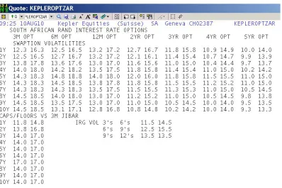
Figure 4. A Reuter’s page for at the money volatility quotes for caps/floors,
caplet/floorlets (IRG means interest rate guarantee), and swaptions. In the swap-tion matrix the columns indicate the tenor of the opswap-tion, the rows indicate the tenor of the into swap that is created if the swaption is exercised. If we had differ-ent strikes as well, then we would have the ‘vol cube’: option tenors, into tenors, strikes, and then the implied volatility at each point in the cube.
6.1. Valuation. The value of the swaption per unit of nominal is [Hull,2005,§26.4]
Vη = Lη[f N(ηd1)−LKN(ηd2)]
(36)
d1,2 =
lnLf
K ± 1 2σ
2t 0
σ√t0
(37)
whereη= 1 stands for a payer swaption,η =−1 for a receiver swaption. Hereσis the volatility of the fair forward swap rate, and is an implied variable quoted in the market.
6.2. Greeks. We will use the following: ∂
∂rZ(0, t) =−tZ(0, t)
∂L ∂r =
n X
i=1
−tiαiZ(0, ti)
∂2L
∂r2 = n X
i=1
t2iαiZ(0, ti)
∂L ∂τ =
n X
i=1
−riαiZ(0, ti)
∂ ∂rd1=
∂ ∂rd2 =
∂f ∂r
1 f σ√t0
∂ ∂σd1=
∂ ∂σd2+
√ t0
∂ ∂τd1=
∂ ∂τd2+
σ 2√t0
Also, if we have a function gh((r,τr,τ)) , then
g
h 0
=g0h−1−gh−2h0
g
h 00
=−2g0h−2h0+g00h−1+ 2gh−3(h0)2−gh−2h00
where the differentiation is with respect tor.
6.2.1. Delta.
∆ =ηN(ηd1)
(38)
6.2.2. pv01.
∂V ∂r =η
∂L
∂r [f N(ηd1)−rKN(ηd2)] +ηL ∂f
∂rN(ηd1) +f N 0(ηd
1)η
∂d1
∂r −rKN 0(ηd
2)η
∂d2
∂r
=η∂L
∂r [f N(ηd1)−rKN(ηd2)] +ηL ∂f
∂rN(ηd1) (39)
Then pv01 = 1 10000
∂V ∂r.
6.2.3. Gamma.
∂2V
∂r2 = η
∂2L
∂r2 [f N(ηd1)−rKN(ηd2)] +η
∂L ∂r
∂f
∂rN(ηd1) +f N 0(ηd
1)η
∂d1
∂r −rKN 0(ηd 2)η ∂d2 ∂r +η∂L ∂r ∂f
∂rN(ηd1) +ηL
∂2f
∂r2N(ηd1) + ∂f ∂rN 0(ηd 1)η ∂d1 ∂r
= η∂
2L
∂r2 [f N(ηd1)−rKN(ηd2)] + 2η ∂L
∂r ∂f
∂rN(ηd1) +ηL ∂2f
∂r2N(ηd1) + ∂f ∂rN 0(ηd 1)η ∂d1 ∂r (40) 6.2.4. Vega. ∂V
∂σ = Lη
f N0(ηd1)η
∂d1
∂σ −rKN 0(ηd
2)η
∂d2
∂σ
= Lf N0(d1)
√ τ (41)
7. Why Black is useless for exotics
In each Black model for maturity dateT, the forward rates will be log-normally distributed in what is called theT-forward measure, whereT is the pay date of the option. The fact that we can ‘legally’ discount the expected payoff under this measure using today’s yield curve is a consequence of some profound academic work ofGeman et al.[1995], which establishes the existence of alternative pricing measures, and the ways that they are related to each other. This paper is very significant in the development of the Libor Market Model.
We can use Black’s model without knowing any of the theory ofGeman et al.[1995]; however, the Black model cannot safely be used to value more complicated products where the payoff depends on observations at multiple dates. For this an alternative model which links the behaviour of the rates at multiple dates will need to be used.
For this, the most universal approach is the Libor Market Model. Here inputs are all the Black models as well as a correlation structure between all the forward rates. From a properly calibrated LMM, one recaptures (up to the calibration error) the prices of traded caplets, caps, and swaptions. However, this calibration can be difficult. It then requires Monte Carlo techniques to value other derivatives.
An intermediate approach is the use of a more parsimonious model with just one driving factor -the so-called single-factor models.
8. Exercises
(1) A company caps three-month JIBAR at 9% per annum. The principal amount is R10 million. On a reset date, namely 20 September 2004, three-month JIBAR is 10% per annum.
(a) What payment would this lead to under the cap? (b) When would the payment be made?
(c) What is the value of the payment on the reset date?
(2) Use Black’s model to value a one-year European put option on a bond with 9 years and 11 months to expiry. Assume that the current cash price of the bond is R105, the strike price (clean) is R110, the one-year interest rate is 10%, the bond’s price volatility measure is 8% per annum, and the coupon rate is 8% NACS.
(3) Consider an eight-month European put option on a Treasury bond that currently has 14.25 years to maturity. The current cash bond price is$910, the exercise price is$900, and the volatility measure for the bond price is 10% per annum. A semi-annual coupon of$35 will be paid by the bond in three months. The risk-free interest rate is 8% for all maturities up to one year.
(a) Use Black’s model to determine the price of the option. Consider both the case where the strike price corresponds to the cash price of the bond and the case where it corre-sponds to the clean price.
(b) Calculate delta, gamma (both with respect to the bond priceB) and vega in the above problem when the strike price corresponds to the quoted price. Explain how they can be interpreted.
(4) Using Black’s model calculate the price of a caplet on the JIBAR rate. Today is 20 Sep-tember 2004 and the caplet is the one that corresponds to the 9x12 period.
Interest-rate volatility is 15%.
Also calculate delta, gamma (both with respect to the 9x12 forward rate) and vega in the above problem.
(5) Suppose that the yield,R, on a discount bond follows the process
dR=µ(R, t)dt+σ(R, t)dz
where dz is a standard Wiener process under some measure. Use Ito’s Lemma to show that the volatility of the discount bond price declines to zero as it approaches maturity, irrespective of the level of interest rates.
(6) The price of a bond at timeT,measured in terms of its yield, isG(yT).Assume geometric Brownian motion for the forward bond yield,y,in a world that is forward risk-neutral with respect to a bond maturing at time T. Suppose that the growth rate of the forward bond yield isαand its volatility isσy.
(a) Use Ito’s Lemma to calculate the process for the forward bond price, in terms ofα, σy, yandG(y).
(b) The forward bond price should follow a martingale in the world we are considering. Use this fact to calculate an expression forα.
(c) Assume an initial value of y =y0. Now show that the expected value of y at time T
can be directly calculated from the above expression. (7) Consider the following quarterly data:
1 2 3 4 5 6 7 8
zero 8.00% 8.50% 8.30% 8.00% 8.00% 8.20% 8.25% 8.40%
vol 17.00% 16.00% 17.00% 16.00% 15.00% 15.00% 14.00% Time here is modified following quarterly.
The volatility data represents the volatility of the all in price for a bond option on the r153 that expires at that time.
The details of the r153 are as follows:
Bond Name Maturity Coupon BCD1 BCD2 CD1 CD2
R153 2010/08/31 13.00% 821 218 831 228
(The BCD details of all r bonds have changed.)
Today is 29 August 2004 and the all in price is 1.1010101.
Price a vanilla European bond option, with a clean price strike, with expiry 30 May 2005, according to Black’s model.
Bibliography
Fischer Black. The pricing of commodity contracts. Journal of Financial Economics, 3:167–179, 1976. 2
Damiano Brigo and Fabio Mercurio. Interest Rate Models - Theory and Practice: With Smile, Inflation and Credit. Springer Finance, second edition, 2006. 8
H. Geman, N. El Karoui, and J. Rochet. Changes of numeraire, changes of probability measure and option pricing. Journal of Applied Probability, 32, 1995. 13
John Hull. Options, Futures, and Other Derivatives. Prentice Hall, sixth edition, 2005. 2, 3,11
Peter J¨ackel. Monte Carlo Methods in Finance. Wiley, 2002. 9
Ricardo Rebonato. Modern pricing of interest-Rate derivatives: the LIBOR market model and beyond. Princeton University Press, 2002. 8,9
Ricardo Rebonato. Volatility and Correlation: The Perfect Hedger and the Fox. Wiley Finance, 2004. 8,10
Financial Modelling Agency, 19 First Ave East, Parktown North, 2193, South Africa.