Continuous Model Reference Adaptive Control with Sliding Mode for a
Class of Nonlinear Plants with Unknown State Delay
Boris Mirkin, Per-Olof Gutman and Yuri Shtessel
Abstract— In this paper, we develop a model reference adap-tive control (MRAC) scheme with sliding mode for a class of nonlinear dynamic systems with state delay which is robust with respect to an unknown plant delay, to a nonlinear perturbation, and to an external disturbance with unknown bounds. A novel Lyapunov-Krasovskii type functional is introduced to design the adaptive controller with smooth control action, and the stability proof.
I. INTRODUCTION
The robust sliding mode control technique applied to uncertain systems with time-delays is a research area that is receiving considerable attention during the last few years, see e.g. [1], [2], [3], [4], [5] and the references therein.
The use of conventional pure robust sliding mode control for plants with delays entails two well-known drawbacks connected to the sliding mode approach itself, namely: (i) all uncertainty bounds need to be available to the designer in advance, and this knowledge is a necessary condition for the closed-loop stability proof; (ii) the control is in general discontinuous, since the control law contains the sign function, and hence, the direct application of such a sliding mode controller may give rise to undesirable chattering.
The relaxation of the first shortcoming of the pure sliding control method motivates the combination of sliding mode robust control with adaptive approaches, whereby the knowl-edge of the upper bounds of the perturbations will not be required. The adaptive approaches may offer an effective tool to solve this problem. Only few combined adaptive—sliding mode results for delay systems have been published, see e.g. [6], [7], [8], [9], [11].
In [6] an adaptive state feedback robust stabilization problem is considered for a class of state delay systems with input nonlinearities. But also that paper restrictively assumes that the adaptive controllerknowsthe bounds of the non-linear perturbation terms, and the bounds of the sector in which the input non-linearity resides. [7] deals with the state feedback stabilization of linear systems with known state delays, subject to bounded external disturbance with unknown bounds. The design guarantees convergence to a small ball. In [8] the variable structure MRAC problem is
This work was supported by the USA-Israel Binational Science Foun-dation under Grant 2006351, and by the Israel Science FounFoun-dation under Grant 588/07.
B. Mirkin and Per-Olof Gutman are with the Faculty of Civil and Environmental Engineering, Technion – Israel Institute of Technology, Haifa 32000, Israel.(bmirkin),(peo)@technion.ac.il
Y. Shtessel is with the Department of Electrical and Computer Engi-neering, The University of Alabama in Huntsville, 301 Sparkman Drive, Huntsville, Alabama [email protected]
considered for a class of stable, input delayed plants. A state feedback stabilizing memoryless controller for linear systems with known parameter matrices in the presence of unknown norm-bounded delayed nonlinear perturbation was studied in [9]. A backstepping method was used to construct the controller.
Discontinuous sliding mode coordinated adaptive decen-tralized tracking for a class of nonlinear systems with state delays was considered in [10], but under the restrictive assumption that the controller knows the time delays.
In our recent paper [11], a sliding mode discontinuous model reference adaptive control (MRAC) scheme was con-sidered for a class of nonlinear dynamic systems which is robust with respect to an unknown state delay, to a nonlinear perturbation, and to an external disturbance with unknown bounds.
From the previous discussion, one can conclude that also in the adaptive case the discontinuous character of the control action is not avoided, and that may not be desirable because of chattering. Practical and efficient approaches to overcome chattering have been reported based mainly on some approximation of the sign function see, e.g. [17]. Then the trajectory will remain in some neighbourhood of the sliding surface, thus decreasing the tracking accuracy. The designer has to trade-off chattering against tracking accuracy. In order to alleviate chattering, higher order sliding mode (HOSM) control that is able to generate robust contin-uous/smooth control actions was proposed in [12], [13], [14]. Both classical SMC and HOSM control are robust to unknown bounded disturbances with known bounds. As we mentioned above, there exist high frequency switching classical SMC algorithms with adaptation that address the problem of unknown bounds of the disturbances. However, we are not aware of smooth/continuous classical SMC or HOSM control that is able to provide adaptation to the unknown bounds of the disturbances especially for nonlinear systems with unknown time delays. Therefore, the design of adaptive continuous SMC that is robust to disturbances with unknown bounds for systems with unknown time delays is a challenge.
In the present paper we extend the result of [11] to the case of smooth control action with sliding mode. We introduce a new continuous adaptive robust tracking scheme for a class of nonlinear dynamic systems with state delay. The proposed adaptive controller parametrization admits model reference adaptive designs with zero asymptotical errors, without knowledge of the time delay, and with robustness properties with respect to state dependent delayed nonlinear
2009 American Control Conference
Hyatt Regency Riverfront, St. Louis, MO, USA June 10-12, 2009
perturbations, also in the presence of an unknown distur-bance. Some cases of a priori knowledge about the state dependent delayed non-linearity are considered.
II. PLANT MODEL AND PROBLEM FORMULATION We consider a class of nonlinear uncertain systems with state delays, suitably initialized, of the form
˙
x(t) =Ax(t) +bu(t) +b f(x(t),x(t−τ),t) +bd(t) (1) wherex∈Rnis the state vector,u(t)∈Ris the control input, andd(t)∈Ris a bounded disturbance. The constant matrices A∈Rn×n and b∈Rn have unknown elements. f(x(t),x(t−
τ),t) is regarded as anuncertain state dependent nonlinear perturbation.τ∈R+is an unknowntime delay.
Our objective is to design a state feedback controller for (1) such that the closed-loop system is stable, and the states x(t)asymptotically exact track the states of the non-delayed stable reference model
˙
xr(t) =Arxr(t) +brr(t) (2) wherexr(t)∈Rnis the state vector, andr∈Ris the reference
input which is assumed to be a uniformly bounded and piecewise continuous function of time. The matrices Ar,br are known constant matrices of appropriate dimensions.
The following is assumed regarding the plant and the reference model:
(A1)There exist anunknownconstant vectorθe∗∈Rnand a nonzero constant scalarθosuch that the following equations are satisfied,
A=Ar−bθe∗T, br=bθo. (3)
(A2) The sign of θo is known and, without loss of generality, positive.
(A3) The external disturbance d(t) is bounded by an unknownconstantkd(t)k<d∗.
(A4)For the nonlinear perturbation f(x(t),x(t−τ),t)we assume that the nonlinear function f(x(t),x(t−τ),t)is such that there exist nonnegative, but unknown, numbersξ1∗l and ξ2∗l such that
|f(x(t),x(t−τ),t)| ≤ξ1∗kx(t)k+ξ2∗kx(t−τ)k (4) III. ADAPTIVECONTROLLERDESIGN
The following procedure of design acontinuousadaptive control was inspired by an idea from conventional sliding mode theory for discontinuous control, see e.g. [18], [17]. A. Sliding surface
First, we definite a sliding surface in the conventional way: S(t) =Ge(t) =0, G=bTrP (5) wheree(t) =x(t)−xr(t)is the tracking error.
The vector G defines a stable sliding motion, where the matrix 0<PT =P∈Rn×n is obtained by solving the Lyapunov equation
PAr+ATrP+Q=0 (6)
for any chosen constant matrixQ∈Rn×nsuch thatQ=QT>
0. Different choices ofQwill not affect boundedness and the asymptotic behavior of the closed loop signals, but they will affect the transient responses in the sliding mode, see e.g. [18], [17].
B. Control law parametrization
The objective is now to propose an adaptive control law such that: (i) all signals in the closed-loop system are bounded; (ii) the tracking error e(t) converges to zero asymptotically with time for any bounded reference input r(t).
We look for a control law parametrization of the form u(t) =θeT(t)e(t) +θI(t) (7) with the updating laws
˙
θe(t) =−ΓS(t)e(t) ˙
θI(t) =−γS(t), θI(0) =0 (8) where θe(t)∈Rn and θI(t)∈R are the vector and scalar
adaptation gains,Γ=ΓT >0 and γ>0 are some constant design matrix and scalar respectively.
Remark 1: The controller has a simple and conceptually clear structure, uses feedback action only, and thus does not require a direct measurement of the command signals as is usually the case in MRAC.
C. Basic tracking error
Next, it is necessary, as always in model reference adaptive control (MRAC) theory [15], [16], to express the closed-loop system in terms of the tracking errore(t) =x(t)−xr(t), and some parameter errors.
In view of (1), (2) and Assumptions (A1) and (A2) we obtain, after some manipulations,
˙
e(t) =Are(t)−bθe∗Te(t)−bθe∗Txr(t)−brr(t)
+b f(x(t),x(t−τ),t) +bd(t) +bu(t) (9) Then by using (7) and in view that br=bθ0, see As-sumption (A1), we have the following basic tracking error equation
˙
e(t) =Are(t) +brθo−1θ˜eT(t)e(t) +brθo−1θI(t)−brr(t)
−brθo−1θ
∗T
e xr(t) +brθo−1f(?) +brθo−1d(t) (10) The parameter error ˜θe(t)∈Rnis
˜
θe(t) =θe(t)−θe∗ (11) with the unknown vectorθe∗ from (A1).
D. The Lyapunov-Krasovskii functional
For stability analysis the following Lyapunov-Krasovskii functional is proposed
V =V1+V2+V3; V1=S2(t) +eT(t)Pe(t) +
Z t
t−τν ke(t)k2
V2=coθo−1z˜T(t)Γ−1z˜(t) V3=coθo−1γ
−1
θI(t)−θI∗sgn(S(t)
2
where
˜
z(t) =θ˜e(t) +z0, zo=2θcooρPbr (13) and the scalar design parameterγ>0. The matrixPis from (6) and co=bTrPbr+1. The constantsν>0,ρ>0 andθI∗ will be defined later. The sign k?k denotes the Euclidian norm. The sign function sgn(S(t))of a signalS(t)is defined as
sgn(S(t)) =
1, S(t)>0; 0, S(t) =0;
−1, S(t)<0.
Remark 2: The main feature and difference from tradi-tional Lyapunov-Krasovskii functradi-tionals used in sliding mode adaptive design is the simultaneously occuring terms based on the error norm and the norm ofS(t). It will be shown that such a combination makes it possible to get smooth control action.
E. The Lyapunov-Krasovskii functional derivatives
Invoking (3), (5) andPfrom Lyapunov’s equation (6), the time derivative ofV1along (10) can be written as
˙
V1(t)|(10)=−eT(t)Qe(t) +2eT(t)PbrbTrPAre(t)
+2coθo−1S(t)θ˜eT(t)e(t) +2coθo−1S(t)θI(t)
+νke(t)k2−νke(t−τ)k2−2coS(t)r(t)
−2coθo−1S(t)θe∗Txr(t) +2coθo−1S(t)d(t) +2coθo−1S(t)f(x(t),x(t−τ),t) (14) Using the inequality from (A4) and boundedness of the reference signals (|r(t)| ≤r∗,kxrk ≤x∗r) we can write the following estimates for some terms of (14)
−2coθo−1S(t)θ
∗T
e xr(t)≤2co|S(t)|θo−1|S(t)| kθ
∗
ek kxr(t)k
≤2co|S(t)|θo−1µ1 (15)
−2coS(t)r(t)≤2co|S(t)| |r(t)|
≤2coθo−1|S(t)|µ2 (16)
2coθo−1S(t)d(t)≤2coθo−1|S(t)| |d(t)|
≤2coθo−1|S(t)|µ3 (17)
2coθo−1S(t)f(?)≤2 ˆξ1|S(t)| ke(t)k +2 ˆξ2|S(t)| ke(t−τ)k
+2coθo−1|S(t)|µ4 (18)
2eT(t)PbrbTrPAre(t)≤ξ3ˆ ke(t)k2 (19) whereµ1=kθe∗kxr∗,µ2=θor∗,µ3=d∗, µ4= ξ1∗+ξ2∗x∗r,
ˆ
ξ1=θo−1coξ1∗, ˆξ2=θo−1coξ2∗ and ˆξ3=2PbrbTrPAr
.
By using (15) - (19) we have from (14) ˙
V1(t)|(10)≤ −eT(t)Qe(t) +ξ3ˆ ke(t)k2+νke(t)k2
−νke(t−τ)k2+2coθo−1S(t)θ˜eT(t)e(t) +2coθo−1S(t)θI(t) +2|S(t)|ξ1ˆ ke(t)k +2|S(t)|ξ2ˆ ke(t−τ)k −2coθo−1|S(t)|θI∗
−ρ|S(t)|2+ρ|S(t)|2 (20)
where−θI∗=µ1+µ2+µ3+µ4.
For convenience, let Q from (6), ν from (12) and ρ from (20) be Q=q1I+q2I,ν=ν1+ν2, ρ=ρ1+ρ2+ρ3, where q1, q1, ν1, , ρ1, ρ2 and ρ3 are positive constants and I is the identity matrix. Then, combining −ρ2|S(t)|2 and 2|S(t)|ξˆ1ke(t)k,−ρ3|S(t)|2and the 2|S(t)|ξˆ2ke(t−τ)k terms of (20), completing the squares, and dropping negative terms, we obtain from (20)
˙
V1(t)|(10)≤ −q1ke(t)k2−ν1ke(t−τ)k2−ρ1|S(t)|2
−q2ke(t)k2+ξ3ˆ ke(t)k2+νke(t)k2+2 ˆξ 2 1
ρ2 ke(t)k
2
−νke(t−τ)k2+2 ˆξ 2 2
ρ3 ke(t−τ)k
2+
ρ|S(t)|2
+2coθo−1S(t)θ˜eT(t)e(t) +2coθo−1S(t)θI(t)
−2coθo−1|S(t)|θI∗ (21)
Let us select values ofρ2,ρ3,q2andν2from the inequalities ρ2(q2−ξ3ˆ −ν)>2 ˆξ12, ρ3ν2>2 ˆξ22 (22) Then we obtain from (21)
˙
V1(t)|(10)≤ −q1ke(t)k2−ν1ke(t−τ)k2−ρ1|S(t)|2
−2coθo−1|S(t)|θI∗+ρ|S(t)|2
+2coθo−1S(t)θ˜eT(t)e(t) +2coθo−1S(t)θI(t) (23) In view of (8) and (13), the time derivative ofV2 satisfies ˙
V2(t)|(10)=2co|θo|−1θ˜e(t)TΓ−1θ˙˜e(t) +2co|θo|−1zToΓ−1θ˙˜e(t)
=−2coθo−1θ˜eT(t)S(t)e(t)−ρ|S(t)|2 (24) For the time derivative ofV3we have
˙
V3(t)|S(t)=6 0=−2coθo−1S(t)θI(t) +2coθo−1|S(t)|θI∗ ˙
V3(t)|S(t)=0=0 (25) Then, invoking (23), (24) and (25) we obtain for the time derivative ofV from (12)
˙
V(t)|S(t)6=0≤ −q1ke(t)k2−ν1ke(t−τ)k2−ρ1|S(t)|2 ˙
V(t)|S(t)=0≤ −q1ke(t)k2−ν1ke(t−τ)k2 (26) This implies that V and, therefore e(t),S(t),θ˜e(t),θe(t),θ˜I(t),θI(t) ∈ L∞ and e(t) ∈ L2 by following the usual arguments in e.g. [15], [16]. The remainder of the stability analysis follows directly using the steps in [15], [16]. Because e(t), θe(t) and θI(t) are bounded it following that u(t) from (7) that u(t)∈L∞.
Furthermore, xr(t),e(t)∈L∞ imply that x(t)∈L∞. Because
x(t)∈L∞ and from Assumption (A4) the function f(?) is
bounded. So all signals are bounded before the controlled system enters the surfaceS(t) =0.
Now we show that limt→∞S(t) =0. Because all the signals
in the right-hand side of (10) are bounded, from (5) we have that ˙S(t) =brPe˙(t)∈L∞and thereforeS(t)is uniformly
continuous. After integration the equation (26) for S(t)6=0 can be rewritten as
Z t
t0
and
Z ∞
t0
|S(t)|2dt≤V(t0)−V∞<∞, (28)
i.e., S(t)∈L2. Using S(t),S˙(t)∈L∞, S(t)∈L2 and e.g. applying Lemma 2.14 [16, p.80] we haveS(t)→0 ast→∞. A similar argument gives thate(t)→0 ast→∞.
Remark 3: We note that the coefficientsρandνfrom (12) are used only for analysis and do not influence the control law. The controller gains adjust automatically to counter the non-desirable effects of the delayed states, the nonlinearity, the disturbance, and parameter uncertainties.
F. Main result
The above arguments constitute the proof of the following result
Theorem 1: Consider system (1) and the reference model (2). Suppose that assumptions (A1)-(A4) hold. Then the adaptive law (7) with update law (8) assures that all signals in the closed-loop plant are bounded and the tracking errore(t) converges to zero asymptotically with time for any reference inputr(t)∈L∞.
Remark 4: Theorem 1 shows that the stability of the closed-loop system and the controller parameters are com-pletely independent of the value of the plant time-delay τ. The controller is also robust to an external disturbance.
IV. SOME EXTENSIONS
We now briefly consider some possible extensions of the above design procedure with the new MRAC scheme. A. The case with multiple and time-varying delays
This paper considers uncertain dynamical systems with one constant time delay. Note that in light of the stability proofs, the method developed here is also applicable to systems with multiple and time-varying delays. In the case of a time-varying delay τ(t), it is required that τ(t)≤τ∗ whereτ∗ is anunknown constant. In this case the adaptive control law remains the same: only a slightly modified form of the Lyapunov-Krasovskii functional (12) is required in the above design procedure.
B. Another `a priori knowledge about nonlinear term We consider e.g., the case of a priori knowledge about a nonlinear term of the form
|f(x(t),x(t−τ),t)| ≤θρ∗ρ(x,t), for all(t,x(t)) whereρ(x,t)is a known bounded continuous positive scalar valued function, andθρ∗is a nonnegative unknown scalar.
In this case the design procedure remains the same as above, but we look for a control law parametrization of the form
u(t) =θeT(t)e(t) +θI(t) +θρ(t)ρ(x,t) (29)
with the updating laws forθe(t)andθI(t)from (8) and
˙ θρ(t) =
−γ2S(t)ρ(x,t), S(t)6=0;
0, S(t) =0. θρ(0) =0 (30)
One can see that the control in (7) is modified by adding a special termθρ(t)ρ(x,t)with the adaptive gain θρ(t) from
(30). For the proof we use a functional of the same type as (12) but with a modification of V3 by adding the term coθo−1γ
−1
2 θρ(t)−θρ∗sgn(S(t)
2
.
C. Nonlinear uncertain systems without delays
Even in the absence of an unknown state delay, the results of the paper are new. For this case, consider e.g. a class of uncertain nonlinear systems of the form (1) but without the time delay, i.e.
˙
x(t) =Ax(t) +bu(t) +b f(x(t),t) +bd(t) (31) and Assumption (A4) is e.g. exchanged for
|f(x(t),t)| ≤ξ1∗kx(t)k (32) with unknownξ1∗. The adaptive control law remainsexactly the sameas (7). The design procedure also remains the same, but instead of the Lyapunov-Krasovskii functional (12), we need to use the Lyapunov like function
V=V1+V2+V3; V1=S2(t) +eT(t)Pe(t) V2=coθo−1z˜T(t)Γ−1z˜(t)
V3=coθo−1γ
−1
θI(t)−θI∗sgn(S(t)
2
(33) V. SIMULATION EXAMPLE
To illustrate the application of the proposed adaptive scheme, let us consider a plant defined by
˙ x(t) =
0 1
−0.9 2
x(t) +
0 3
u(t) +sin(t)
+cos(x1(t−τ))x2(t) +sin(x2(t−τ))x1(t) x(s) =[0 0]T,s∈[−τ0), x(0) = [−1 −1]T (34) To build the adaptive controller we choose the reference model
˙ xr(t) =
0 1
−2 −3
xr(t) +
0 2
r(t)
xr(0) = [0 0]T (35)
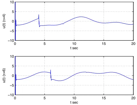
In this example all the parameters includingτ are unknown to the controller. The only information available to the controller is the structural information given in Assump-tions A1– A4. The parameter values of the controller are Γ=200I and γ =200. The reference input is r(t) =2+ 1.5sin(0.5t)rad/sec.
0 5 10 15 20
−1.5
−1
−0.5 0 0.5 1 1.5
e(t) (
!
=4)
t sec
0 5 10 15 20
−1.5
−1
−0.5 0 0.5 1 1.5
e(t) (
!
=6)
[image:5.612.63.287.64.238.2]t sec
Fig. 1. Simulation of the adaptive control system for the nonlinear plant with unknown state delay. The graphs show the time history of the tracking errore(t) = [e1(t),e2(t)]Tfor the two values of the state delay, respectively.
0 5 10 15 20
−10
−5
0 5 10
u(t) (
!
=4)
t sec
0 5 10 15 20
−10
−5
0 5 10
u(t) (
!
=6)
t sec
Fig. 2. Simulation of the adaptive control system for the nonlinear plant with unknown state delay. The graphs show the time history of the control
u(t)for the two values of the state delay, respectively.
VI. CONCLUDING REMARKS
A systematic design procedure is proposed for design of new direct adaptive model reference adaptive control schemes for a class of uncertain nonlinear state delay systems with an unknown state delay and an external disturbance. It was shown that using novel adaptive controller parameter-izations it is possible to design a state feedback controller withsliding mode and smooth control action, which ensures the boundedness of the closed-loop signals, exact asymptotic tracking, and robustness with respect to two cases of non-linear state dependent perturbations, an external disturbance, and a state delay. The main advantage of the new scheme when applied to a considered class of nonlinear systems: (i) its conceptual clarity and simplicity; (ii) it guarantees smooth control action; (iii) its stability proof, based on a
−1.2 −1 −0.8 −0.6 −0.4 −0.2 0 0.2
−1.5 −1 −0.5 0 0.5 1 1.5 2 2.5 3 3.5
e2
(
!
=4)
e1 (!=4)
G=[2.5 1]
[image:5.612.320.546.65.238.2]G=[2 1]
Fig. 3. Simulation of the adaptive control system for the nonlinear plant with unknown state delay. The graphs show the time history of the tracking errorse1(t)ande2(t)in the phase plane for the two values of the vector G, respectively.
−1.5 −1 −0.5 0 0.5 1 1.5
−3 −2 −1 0 1 2 3
e2
(
!
=4)
e1 (!=4)
G=[2 1]
Fig. 4. Simulation of the adaptive control system for the nonlinear plant with unknown state delay. The graphs show the time history of the tracking errorse1(t)ande2(t)in the phase plane. Two trajectories starting from two different initial conditions are plotted.
straightforward Lyapunov arguments, is particularly simple. A suitably selected new Lyapunov-Krasovskii type func-tional is proposed to design the update mechanism for the controller parameters, and to prove stability. Simulations demonstrate that the MRAC controller with sliding mode and smooth control action has good tracking performance and robustness.
[image:5.612.62.288.310.483.2] [image:5.612.326.546.321.496.2]0 5 10 15 20 −25
−20 −15 −10 −5 0
!e
(t) (
"
=4)
[image:6.612.64.287.65.238.2]t sec
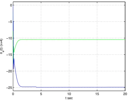
Fig. 5. Simulation of the adaptive control system for the nonlinear plant with unknown state delay. The graphs show the time history of the adjusted parameters vectorθe(t).
REFERENCES
[1] N. Luo, M. de la Sen, and J. Rodellar, “Robust stabilization of a class of uncertain time delay systems in sliding mode,”Int. J. Robust Nonlinear Control, vol. 144, no. 7, pp. 59–74, 1997.
[2] R. El-Khazali, “Variable structure robust control of uncertain time-delay systems,”Automatica, vol. 34, no. 3, pp. 327–332, 1998. [3] F. Gouaisbaut, Y. Blanco, and J. P. Richard, “Robust sliding mode
control of non-linear systems with delay: a design via polytopic formulation,”International Journal of Control, vol. 77, no. 2, pp. 206– 215, 2004.
[4] Y. Xia and Y. Jia, “Robust sliding-mode control for uncertain time-delay systems: An LMI approach,”IEEE Transactions on Automatic Control, vol. 48, pp. 1086–1092, 2003.
[5] Y. Shtessel, A. Zinober, and I. Shkolnikov, “Sliding mode control for nonlinear systems with output delay via method of stable system center,”Journal of Dynamic Systems, Measurement, and Control, vol. 125, pp. 253–257, 2003.
[6] J. Yan, “Sliding mode control design for uncertain time-delay systems subjected to a class of nonlinear inputs,” Int. J. Robust Nonlinear Control, vol. 13, p. 519532, 2003.
[7] S. Oucheriah, “Adaptive variable structure control of linear delayed systems,” Journal of Dynamic Systems, Measurement, and Control, vol. 127, pp. 710–714, 2005.
[8] E. Mirkin, “Variable structure model reference adaptive control with an augmented error signal for input-delay systems,” inPhysCon 2005, St. Petersburg, Russia, 2005.
[9] Ch. Hua, Q. Wang and X. Guan, “Adaptive backstepping control for a class of time delay systems with nonlinear perturbations.”
International Journal of Adaptive Control and Signal Processing, vol. 22, no. 7, pp. 289–305, 2008.
[10] B. M. Mirkin, E. L. Mirkin, and P. O. Gutman, “Sliding mode coordinated decentralized adaptive following of nonlinear delayed plants,” inProc. of the International Workshop on Variable Structure Systems, Alghero, Italy, June 5-7, 2006, pp. 244–249.
[11] B. Mirkin, P-O. Gutman and Y. Shtessel, “Sliding Mode Adaptive Following of Nonlinear Plants with unknown State Delay,” in Proc. of the 10-th International Workshop on Variable Structure Systems, Antalya, Turkey, June 8-10, 2008, pp. 244–249.
[12] A. Levant, “High-order sliding modes: differentiation and output-feedback control.”International Journal of Control, vol. 76, no. 9-10, pp. 924–941, 2003.
[13] Y. Shtessel, I. Shkolnikov and M. Brown, “An Asymptotic Second Order Smooth Sliding Mode Control.”Asian Journal of Control, vol. 5, no. 4, pp. 498–504, 2003.
[14] Y. Shtessel, I. Shkolnikov and A. Levant, “Smooth Second Order
Sliding Modes: Missile Guidance application.” Automatica, vol. 43, no. 8, pp. 1470–1476, 2007.
[15] P. A. Ioannou and J. Sun,Robust Adaptive Control. New Jersey: Prentice-Hall, 1996.
[16] G. Tao, Adaptive Control Design and Analysis. New York: John Wiley, 2003.
[17] J. Y. Hung, W. Gao, and J. C. Hung, “Varibale structure control: A survey,”IEEE Transactions on Industrial Electronics, vol. 40, no. 1, pp. 2–22, 1993.