Ragweed pollen production and dispersion modelling within a regional climate system, calibration and application over Europe

www.biogeosciences.net/13/2769/2016/ doi:10.5194/bg-13-2769-2016

© Author(s) 2016. CC Attribution 3.0 License.

Ragweed pollen production and dispersion modelling within a

regional climate system, calibration and application over Europe

Li Liu1,2, Fabien Solmon1, Robert Vautard3, Lynda Hamaoui-Laguel3,4, Csaba Zsolt Torma1, and Filippo Giorgi1

1_{Earth System Physics Section, the Abdus Salam International Centre for Theoretical Physic, Trieste, Italy} 2_{Guizhou Key Laboratory of Mountainous Climate and Resources, Guiyang, China}

3_{Laboratoire des Sciences du Climat et de l’Environnement, IPSL, CEA-CNRS-UVSQ, UMR8212, Gif sur Yvette, France} 4_{Institut National de l’Environnement Industriel et des Risques, Parc technologique ALATA, Verneuil en Halatte, France} Correspondence to: Li Liu (liliuliulish@outlook.com) and Fabien Solmon (fsolmon@ictp.it)

Received: 27 August 2015 – Published in Biogeosciences Discuss.: 3 November 2015 Revised: 17 April 2016 – Accepted: 21 April 2016 – Published: 11 May 2016

Abstract. Common ragweed (Ambrosia artemisiifolia L.) is a highly allergenic and invasive plant in Europe. Its pollen can be transported over large distances and has been rec-ognized as a significant cause of hay fever and asthma (D’Amato et al., 2007; Burbach et al., 2009). To simulate production and dispersion of common ragweed pollen, we implement a pollen emission and transport module in the Re-gional Climate Model (RegCM) version 4 using the frame-work of the Community Land Model (CLM) version 4.5. In this online approach pollen emissions are calculated based on the modelling of plant distribution, pollen production, species-specific phenology, flowering probability, and flux response to meteorological conditions. A pollen tracer model is used to describe pollen advective transport, turbulent mix-ing, dry and wet deposition.

The model is then applied and evaluated on a European domain for the period 2000–2010. To reduce the large uncer-tainties notably due to the lack of information on ragweed density distribution, a calibration based on airborne pollen observations is used. Accordingly a cross validation is con-ducted and shows reasonable error and sensitivity of the cal-ibration. Resulting simulations show that the model captures the gross features of the pollen concentrations found in Eu-rope, and reproduce reasonably both the spatial and temporal patterns of flowering season and associated pollen concen-trations measured over Europe. The model can explain 68.6, 39.2, and 34.3 % of the observed variance in starting, cen-tral, and ending dates of the pollen season with associated root mean square error (RMSE) equal to 4.7, 3.9, and 7.0 days, respectively. The correlation between simulated and

observed daily concentrations time series reaches 0.69. Sta-tistical scores show that the model performs better over the central Europe source region where pollen loads are larger and the model is better constrained.

From these simulations health risks associated to common ragweed pollen spread are evaluated through calculation of exposure time above health-relevant threshold levels. The to-tal risk area with concentration above 5 grains m−3takes up 29.5 % of domain. The longest exposure time occurs on Pan-nonian Plain, where the number of days per year with the daily concentration above 20 grains m−3exceeds 30.

1 Introduction

2006; Stach et al., 2007; Smith et al., 2008; Šikoparija et al., 2013).

One of the goals of the project “Atopic diseases in chang-ing climate, land use and air quality” (ATOPICA) (http: //www.atopica.eu) is to better understand and quantify the ef-fects of environmental changes on ragweed pollen and asso-ciated health impacts over Europe. In this context the present study introduces a modelling framework designed to simu-late production and dispersion of ragweed pollen. Ultimately these models can be used for investigating the effects of changing climate and land use on ragweed (Hamaoui-Laguel et al., 2015) and for providing relevant data to health impact investigators.

Presently a number of regional models, mostly designed for air quality prevision, incorporate release and dispersion dynamics of pollen (Helbig et al., 2004; Sofiev et al., 2006, 2013; Skjøth, 2009; Efstathiou et al., 2011; Zink et al., 2012; Prank et al., 2013; Zhang et al., 2014). Methods for produc-ing ragweed pollen emission suitable for input to regional scale models have been developed in recent studies (Skjøth et al., 2010; Šikoparija et al., 2012; Chapman et al., 2014). Due to a lack of statistical information related to plant location and amount within a given geographical area, the bottom up approach to produce plant presence inventories is unpractical for most herbaceous allergenic species like ragweed. Quan-titative habitat maps for such species are often derived from spatial variations in annual pollen sum, knowledge on plant ecology and detailed land cover information by top-down approach (such as Skjøth et at., 2010, 2013; Thibaudon et al., 2014; Karrer et al., 2015). Lately, an observation-based habitat map of ragweed has been published in the context of the ENV.B2/ETU/2010/0037 project “Assessing and control-ling the spread and the effects of common ragweed in Eu-rope” (Bullock et al., 2012). This inventory is further cali-brated against airborne pollen observations to reproduce the ragweed distribution with high accuracy, according to Prank et al. (2013). Recently Hamaoui-Laguel et al. (2015) used the observations collected in Bullock et al. (2012), combined with simplified assumptions on plant density and a calibra-tion using observacalibra-tions to obtain a ragweed density inventory map. This approach made use of the Organising Carbon and Hydrology in Dynamic Ecosystems (ORCHIDEE) and the Phenological Modeling Platform (PMP) for obtaining daily available pollens (potential emissions) in Europe.

On average, one ragweed plant can produce 1.19±0.14 billion pollen grains in a year (Fumanal et al., 2007), but resources available (solar radiation, water, CO2, and nutri-ents) for an individual plant during the growth season could alter its fitness and further influence its pollen production (Rogers et al., 2006; Simard and Benoit, 2011, 2012). Fu-manal et al. (2007) investigate the individual pollen produc-tion of different common ragweed populaproduc-tions in natural en-vironment and propose a quantitative relationship between annual pollen production and plant biomass at the beginning of flowering. This allows to integrate the response of

pro-ductivity to various environmental conditions through land surface model.

The timing of the emission can be estimated from a combi-nation of phenological models and the species specific pollen release pattern driven by short-term meteorological condi-tions (Martin et al., 2010; Smith et al., 2013; Zink et al., 2013). Ragweed is a summer annual, short-day plant. Before seeds are able to germinate, it requires a period of chilling to break the dormant state (Willemsen, 1975). The following growth and phenological development depends on both tem-perature and photoperiod (Allard, 1945; Deen et al., 1998a). Flowering is initiated by a shortening length of day but could be terminated by frost (Dahl et al., 1999; Smith et al., 2013) or drought (Storkey et al., 2014). A number of phenological models have been developed for ragweed, either based on correlation fitting between climate and phenological stages (García-Mozo et al., 2009) or explicitly represented by bio-logical mechanisms (Deen et al., 1998a; Shrestha et al., 1999; Storkey et al., 2014; Chapman et al., 2014). The mechanistic models take into account the responses of development rates to temperature, photoperiod, soil moisture, or stress condi-tion (frost, drought, etc.). Mostly they are based on growth experiments but have to enforce a standard calendar date or a fixed day length for the onset of flowering when they are used in real conditions. While the airborne pollen observa-tions from European pollen monitoring sites have a high year to year, site to site variability. Therefore it might be practi-cal to combine the mechanistic model with correlation fitting when the knowledge of plant physiology and local adaptation of phenology are not sufficiently known at the moment.

In this paper, we present a pollen emission scheme that incorporate plant distribution, pollen production, species-specific phenology, flowering probability distribution, and pollen release based on recent studies. By combining the emission scheme with a transport mechanism a pollen simulation framework within the Regional Climate Model (RegCM) version 4 is then developed to study ragweed pollen dispersion behaviours on a regional scale. In Sect. 2 we provide a description of the RegCM-pollen simulation configuration, emission parameterization details, the pro-cessing of plant spatial density and observations data used for calibration in the study. In Sect. 3 we define the model experiment, explain the method used to calibrate ragweed density, present the simulation results of pollen season, eval-uate the performances of the coupled model system over a recent period covered with observations, and finally present the climatological information about the ragweed pollen risk over European domain on a decadal timescale. Summary and conclusions appear in Sect. 4.

2 Materials and methods

(ICTP) regional climate model, i.e. RegCM4, which has been used for a number of years in a wide variety of applica-tions (Giorgi et al., 2006, 2012; Meleux et al., 2007; Pal et al., 2007). In this framework, we develop a pollen model for ragweed which calculates (i) the seasonal production of pollen grains and (ii) their emission and atmospheric pro-cesses (transport and deposition) determining regional pollen concentrations. As detailed hereafter pollen emission and transport are developed in the preexisting framework of the RegCM atmospheric chemistry module (Solmon et al., 2006, 2012; Zakey et al., 2006; Tummon et al., 2010; Shalaby et al., 2012). Pollen production is developed in the framework of the Community Land Model (CLM) version 4.5 (Oleson et al., 2013), which is the land surface scheme coupled to RegCM. Figure 1 gives an overview of such development framework. In the following subsections, we give details about the important data and steps of the development.

2.1 Observed pollen concentrations

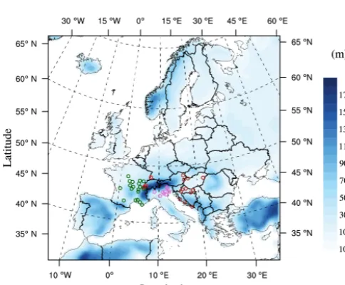
Pollen observations are central for calibration and valida-tion of the pollen module as discussed further. The pollen data are provided by the European Aeroallergen Network (https://ean.polleninfo.eu/Ean/) and affiliated national aer-obiology monitoring network RNSA(France, http://www. pollens.fr/en/), ARPA-Veneto (Italy, http://www.arpa.veneto. it), and Croatian organizations including the Institute of Pub-lic Health, the Department of Environmental Protection and Health Ecology at Institute of Public Health “Andrija Štam-par” and Associate-degree college of Velika Gorica. The archives cover ragweed pollen concentrations (expressed as grain m−3)with daily resolution from 44 observations sta-tions from 2000–2012 year (Table 1). The pollen observa-tion sites range from 42.649 to 48.300◦N and from 0.164 to 21.583◦E. The sites are grouped for study purposes into four regions: France (FR), Italy (IT), Germany–Switzerland (DE+CH) and central Europe (Central EU) including Aus-tria, Croatia, and Hungary (Fig. 2). Ragweed pollens are col-lected at an airflow rate of 10 L min−1using volumetric spore traps based on the Hirst (1952) design. Samples were exam-ined with light microscopy for the identification and counting of pollen grains. The International Association for Aerobiol-ogy (IAA) recommends for the samples reading at magnifi-cation 400×minimum of 3 longitudinal bands or at least 12 transverse bands or minimum 500 random fields (Jäger et al., 1995). The actual sampling methods (longitudinal, transverse or random) and magnifications may vary between the several national networks but are generally compliant (Jato et al., 2006; Skjøth et al., 2010; García-Mozo et al., 2009; Sofiev et al., 2015; Galán et al., 2014; Thibaudon et al., 2014). We based our study on daily pollen concentrations, although for some stations hourly data are available. The observations pe-riod ranges from 2000 to 2012 but for some stations obser-vations only cover part of this period. The obserobser-vations of 2000–2010 are designed for model application and

evalua-tion about ragweed pollen risk. The data for 2011 and 2012 are left and only used for verifying pollen season simulated by a phenology model.

2.2 Model setup

Ragweed pollen simulations are carried out for a European domain ranging from approximately 35 to 70◦N, and from 20◦W to 40◦E (Fig. 2). The horizontal resolution is 50 km, with 23 atmospheric layers from the surface to 50 hPa. Ini-tial and lateral atmospheric boundary conditions are pro-vided by ERA-Interim analysis at 1.5◦ spatial resolution and 6 h temporal resolution. Weekly SSTs are obtained from the NOAA optimum interpolation (OI) SST analysis (with weekly ERA sea surface temperatures). Beside CLM4.5 as a land surface scheme, other important physical options are Holtslag PBL scheme (Holtslag et al., 1990) for boundary layer, Grell scheme (Grell, 1993) over land and Emanuel scheme (Emanuel and Zivkovic-Rothman, 1999) over ocean for convective precipitation, the SUBEX scheme (Pal et al., 2000) for large-scale precipitation. Aerosol and humidity are advected using a semi-Lagrangian scheme. The period 2000– 2010 is chosen for the study. Even though the focus of the study is July–October of flowering season, the model is in-tegrated continuously throughout the year notably for simu-lating ragweed phenology. To compare with the observation described in Sect. 2.1, simulated pollen concentrations time series are interpolated to the station locations and averaged daily.

2.3 Ragweed spatial density

Figure 1. Ragweed pollen modelling within online RegCM-pollen simulation framework.

Figure 2. Model domain and the observation sites with topography.

ability index as

Dp(x, y)=const·H (x, y)·CI(x, y)·

_{K(x, y)}

25

r

. (1)

Here const=0.02 is assumed to be the maximal density (plant m−2)in the most suitable habitats (Efstathiou et al., 2011),H (x, y)taken as the crop and urban lands in CMIP5 land use classification (Hurtt et al., 2006). For countries with low-quality observations or with no available inventories, the detection probability is replaced by the average over neigh-bouring countries with reliable data.

2.4 Parameterization of the pollen emission flux

Pollen emission patterns on regional scale depend on plant density, production, and meteorological conditions. The pa-rameterization of pollen emission flux is a modified version of Helbig et al. (2004). The vertical flux of pollen particlesFp in a given grid cell is assumed to be proportional to the prod-uct of a characteristic pollen grain concentration per plant in-dividualc∗(grain m−3plant−1)and the local friction velocity u∗. This potential flux is then modulated by a plant-specific factorce that describes the likelihood of blossoming, and a meteorological adjustment factor. Finally the flux is scaled up at the grid level using the plant densityDp(plant m−2) discussed previously in Sect. 2.3.

Fp=Dp·ce·Ke·c∗·u∗, (2)

2.5 Pollen production

The characteristic concentrationc∗is related to pollen grain production using

c∗= qp

LAI·Hs, (3)

whereqpis the annual pollen production in grains per individ-ual plant (grains plant−1), LAI=3 is the leaf area index term, andHs=1 is the canopy height (m). These later parameter are determined on the basis of CLM4.5 C3 grass land use categories during summer.

Based on this assumption, qp is calculated following Fu-manal et al. (2007) (Eq. 4). This parameterization integrates the response of pollen grain productivity to various environ-mental conditions affecting C3 grass NPP, including climate variables and atmospheric CO2 concentration for example. It involves a variety of biophysical and biogeochemical pro-cesses at the surface such as photosynthesis, phenology, al-location of carbon/nitrogen assimilates in the different com-ponents of plant, biomass turnover, litter decomposition, and soil carbon/nitrogen dynamics.

log₁₀(qp)=7.22+1.12log₁₀(plant dry biomass) (4) In this approach, yearly total pollen production calculation from mature plant dry biomass needs to be determined in ad-vance, i.e. before integration of the pollen modelling chain. This is done by making a preliminary RegCM-CLM4.5 run with prognostic NPP activated and archived. Alternatively, in order to reduce simulation costs and insure model portabil-ity to other domains we also built a precomputed global C3 grass yearly accumulated NPP data base. This data can be directly interpolated and prescribed to RegCM4 for pollen runs. This global data base is built by running the land com-ponent CLM4.5 of the Community Earth System Model ver-sion 1.2 (CESM1.2) (Oleson et al., 2013) with the Biome-BGC biogeochemical model (Thornton et al., 2002, 2007) enabled and forced by CRUNCEP (Viovy, 2011). We ac-knowledge that NPP obtained this way is not fully consistent with RegCM simulated climate but this approach represents a reasonable and practical compromise.

2.6 Flowering probability density distribution

In Eq. (2),Ceis a probability density function accounting for the likelihood of the plant to flower and effectively release pollen in the atmosphere. The inflorescences of common rag-weed consist of many individual flowers that reach anthesis sequentially (Payne, 1963). At the beginning of the season only a few plants flower and the amount of available pollen grains is small, regardless of the favourable meteorological conditions. The number of flowers increases with time un-til a maximum is reached. Afterwards, the number decreases again until the end of the pollen season. To represent this dy-namic, we use the normal distribution function reported in Prank et al. (2013). The probability distribution of flower-ing time is represented by a Gaussian dependflower-ing on “accu-mulated biological days” BD, and centred midway between flowering starting and ending biological days BDfeand BDfs:

ce=const· 1

σ

√

2π

·e−

(BD−BDfe+BDfs

2 )2

2σ2 _{, (5)}

where const=20×10−4is determined by adjusting the inte-grated amount of pollens between BDfeand BDfsto the total yearly productionqpdetermined from NPP.σis the standard deviation determined by the length of the season, considering

that the season represents about 4 standard deviations of the Gaussian distribution 4σ=BDfe−BDfs. The probability dis-tribution is however set to zero as soon as the daily minimum temperature is below 0◦, considering that first frost set up the end of ragweed activity (Dahl et al., 1999). In the following section we describe how biological days (BD) are effectively determined.

2.7 Phenology representation and flowering season

definition

2.7.1 Biological days

For simulating the timing of the flowering season, we adapt the mechanistic phenology model of Chapman et al. (2014), which is based on growth experiments (Deen et al., 1998a, b, 2001; Shrestha et al., 1999). Phenology is simulated using BD accumulated for the current year of simulation and from the first day (t0)after the spring equinox for which daily min-imum temperature exceeds a certain thresholdTmindefined further (Chapman et al., 2014). BD on timetdepends on key environmental variables through:

BD(T , L, θ )= Z

t0

rT(T )·rL(L)·rS(θ )·dt, (6)

whererT,rL,rS are the response of development rates to temperatureT, photoperiodL, and soil moistureθ, respec-tively. In this approach, biological day varies according to lo-cal climate as illustrated in Sect. 3.2. The phenologilo-cal devel-opment of ragweed before flowering is separated into vegeta-tive and reproducvegeta-tive phases controlled by different factors. Vegetative development stages are germination to seedling emergence (4.5 BD) and emergence to end of juvenile phase (7.0 BD) (Deen et al., 2001). The development rate at the ger-mination to seedling emergence is assumed to be affected by temperature and soil moisture, while the rate at the emer-gence to end of juvenile phase is affected by temperature alone. From the end of the juvenile phase to the beginning of anthesis (13.5 BD) (Deen et al., 2001) the reproductive development phase takes place and is affected by tempera-ture and photoperiod. Vegetative and reproductive processes are assumed to have an identical response to temperature based on the cardinal temperature determined by Chapman et al. (2014).

rT(T )= 

   

   

0 T < Tmin





T−Tmin Topt−Tmin

Tmax−T Tmax−Topt

Tmax−Topt Topt−Tmin



 c

Tmin≤T≤Tmax

0 T > Tmax

,

these parameters are derived from growth trail data (Deen et al., 1998a, b, 2001; Shrestha et al., 1999).

The response of development rates to photoperiod is sim-ulated using a modified version of function presented by Chapman et al. (2014)

rL(L)= (

e(L−14.0)ln(1−Ls) _L≥14.0

1 L <14.0 (8)

whereLis day length, expressed in hours. The photoperiod response delays plant development when the day is longer than the threshold photoperiod fixed to 14.0 h (Deen et al., 1998b).Lsis a photoperiod sensitivity parameter varying be-tween 0 and 1, which controls development delay and can be adjusted according to sensitivity test to reflect ragweed phe-nology adapted to local ecological environment. Photoperi-ods are assumed to affect reproductive development from the end of the juvenile phase.

The response of development rates to soil moisture is as-sumed to occur from the germination to seedling emergence stage. We use a linear function similar to the one used to ac-count for soil moisture impact on biogenic emission activity factor in MEGAN (Guenther et al., 2012)

rS(θ )=   

 

0 θ < θw θ−θw

θopt−θw θw≤θ≤θ1 1 θ > θ1

(9)

whereθis volumetric water content (m3m−3),θw(m3m−3) is wilting point (the soil moisture level below which plants cannot extract water from soil) andθopt(=θw+0.1, m3m−3) is the optimum soil moisture level in the seed zone over which the development rate reaches maximum (Deen et al., 2001).

According to this phenology model, a total of about 25 BD are theoretically needed to reach the beginning of pollen sea-son BDfsfrom the initiation date of BD accumulation. How-ever this model relies on parameters determined from con-trolled conditions and transposition to natural environment is not straightforward in order to calculate a realistic BDfs. Moreover, the model does not allow to calculate a priori the end of season date BDferequired in Eq. (5). While we do rely on BD to represent the pheonolgical evolution within the sea-son, we however constrain the starting and ending biological days of the season (BDfs and BDfe)based on observations, as explained hereafter.

2.7.2 Dates of the flowering season

Experimentally, pollen season can be defined in a number of ways from observed pollen concentrations and listed for ex-ample in Jato et al. (2006). A widely used definition is the period during which a given percentage of the yearly pollen sum is reached. Another definition refers to the period be-tween the first and last day with pollen concentrations

ex-ceeding a specific level. Looking at the temporal distribu-tion of observadistribu-tions, particularly long distribudistribu-tion tails can be found in some cases at the beginning and the end of the pollen season, especially in stations where pollen levels are moderate. This makes the definition of pollen season rather imprecise, while it is in general more constrained in areas with high yearly pollen sum. In our approach, we define the start of the pollen season from 44 observation stations (de-scribed in Sect. 2.1) as the following: the first day of a series of 3 days in a weekly window for which the pollen concen-trations exceed 5 grains m−3, and after 2.5 % of the yearly pollen sum has been reached. The end of the pollen sea-son is defined as the following: the last day of a series of 3 days in a weekly window for which the pollen concentra-tions exceed 5 grains m−3, just before reaching 97.5 % of the yearly pollen sum. (5 grains m−3 is supposed the mini-mum threshold to induce medically relevant risks.) The cen-tre of the pollen season is simply defined as the time when the yearly pollen sum reaches 50 %. Kriging method is then used to spatially interpolate pollen season dates determined for each station over the simulation domain. For each grid cell, BDfs and BDfmare determined by simulating and ac-cumulating biological days up to the experimentally defined starting and mid-season dates. Ending season dates is cal-culated as 2BDfm−BDfsaccording Eq. (5). This methodol-ogy requires again a pre-calculation run of RegCM4/CLM4.5 where simulated BD is output in order to be matched with ob-served season dates for each year. Once this step is achieved, spatially resolved BDfsand BDfecan be obtained by averag-ing across the years and used to perform the integrated pollen run.

2.8 Instantaneous release factor

In Eq. (2), theKe factor accounts for short-term modula-tion of pollen flux from meteorological condimodula-tions. Follow-ing Sofiev et al. (2013) Ke is a function of wind speed, relative humidity, and precipitation calculated by RegCM-CLM45 during the run.

Ke= _h

max−h hmax−hmin

·

fmax−exp

−U+w∗

Usatur

·

_pmax−p

pmax−pmin

(10)

Figure 3. First guess (a) and calibrated (b) ragweed density distribution.

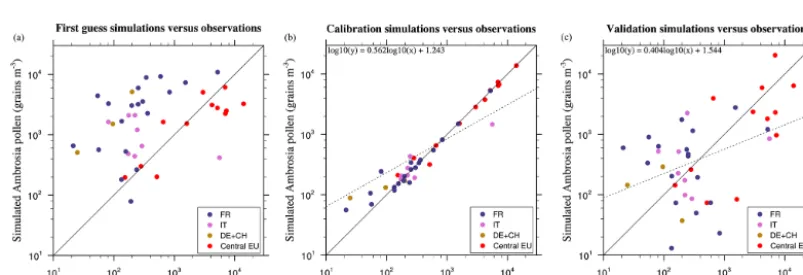
Figure 4. Average (2000–2010) annual pollen sum for first guess (a), calibration (b) and validation (c) simulations on sites.

3 Model application and evaluation

3.1 First guess simulation and calibration of the

ragweed density

A first pollen run is performed using the first guess ragweed density described in Sect. 2 and displayed in Fig. 3a. First guess density map shows maxima of ragweed in the south-east of France, Benelux countries, and central Europe re-gions. When comparing the resulting field to observation, simulated concentrations obtained with the first guess dis-tribution are generally overestimated over France, Switzer-land and Germany, underestimated in parts of central Europe, and have comparable order of magnitude over some Italian and Croatian stations (Fig. 4a). These important biases are in large part due to assumptions made in the construction of the first guess plant density distribution. In order to reduce these biases we perform a model calibration by introducing a correction to the first guess ragweed distribution. For each station, calibration coefficients are obtained by minimizing the yearly root mean square error (RMSE) after constrain-ing the decadal (2000–2010) mean simulated pollen concen-tration to match the decadal mean observed concenconcen-trations

(2000–2010) within an admissible value. Calibration coeffi-cients obtained over each station are then interpolated spa-tially on the domain using ordinary Kriging technique. Then a calibrated simulation using the calibrated density distribu-tion is carried out and repeated several times. After three it-erations, the correlation of yearly totals across observation stations increase from 0.23 to 0.98 and the patterns are clus-tering around the 1:1 line (Fig. 4b).

The final calibrated ragweed distribution (Fig. 3b) shows high density in central Europe including Hungary, Serbia, Bosnia and Herzegovina, Croatia, and western Romania, northern Italy, western France, and also in the southern Netherlands and northern Belgium. The calibration adjusts the density over all the grid cells with ragweed presence by a factor ranging between 0.1 and 4.4 with an average of 0.98.

normalized root mean squared error of 21 % (Fig. 4c). With-out surprise, this is less than when using the full data sets for calibration. In particular a few stations with particularly high concentrations protruding from surrounding sites (for example, ITMAGE and ROUSSILLON) have a large impact on the results of validation. We compared our cross valida-tion (eight or nine sites left out each time) with three papers about ragweed pollen source estimation over the Pannonian Plain, France and Austria (Skjøth et al., 2010; Thibaudon et al., 2014; Karrer et al., 2015). Their cross validations (one site left out each time) show corresponding correlations of 0.37, 0.25, 0.63 and root mean squared error of 25, 16 and 3 %, respectively. Our results are within this range. We agree that caution should be taken in areas without a decent number of station coverage where the calibration cannot be done.

Note that through correction, other systematic sources of errors possibly affecting the modelling chain might also be implicitly corrected, leading to undesirable error compen-sations. However, after running additional tests (not shown here), for example varying model dynamical boundary con-ditions, a relatively small impact on pollen model perfor-mance is found when compared to the ragweed density dis-tribution impact.

3.2 Simulation of pollen season

The simulated starting dates, central dates, and ending dates of pollen season are averaged from 2000 to 2010 and pre-sented in Fig. 5. The pollen season generally shows a posi-tive gradient from the south to the north and from low alti-tude to high altialti-tude, resulting from the combined effects of temperature, day length, and soil moisture. The starting date varies between 21 July and 8 September. Flowering starts in the central European source regions earlier than in west and north of source regions. The central dates are reached be-tween 1 August and 27 September, without noticeable dif-ference between central and west source regions. Flowering ends in the central later than in the west of source regions. The pollen season is longest in the central main source re-gions.

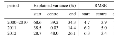
Table 2 lists the statistical correlation between simulated and observed pollen starting, central, and ending dates. The model can reproduce starting and central dates better than ending dates. Goodness-of-fit tests show that the models ac-count for 68.6, 39.2, and 34.3 % of the observed variance in starting, central, and ending dates. The RMSE is 4.7, 3.9, and 7.0 days for the pollen starting, central, and ending dates, respectively. The model reproduces the pollen season in the main source regions fairly well (Table 1), where the aver-aged differences between the simulated and observed pollen season progression are less or equal to 3 days and RMSE is lower than 6 days. For the areas with lower ragweed infes-tation the results vary widely. The starting dates and central dates are still reproduced well for a majority of the stations while the ending dates are more problematic with averaged

Table 2. Statistical correlation between simulated and observed

rag-weed pollen season for fitting 2000–2010 and prediction (2011, 2012).

period Explained variance (%) RMSE

start centre end start centre end

2000–2010 68.6 39.2 34.3 4.7 3.9 7.0 2011 38.5 0.03 14.4 6.2 5.0 8.0 2012 28.7 48.0 26.1 6.3 3.4 8.2

differences above 6–10 days and RMSE over 8–12 days at some stations. This might result from patchy local ragweed distribution and the effect of long-range transport of pollen, which contributes to the determination of pollen season dates and are assumed to be representative of local flowering in our approach. Some stations also stop pollen measurement be-fore the actual end of pollen season which leads to a lower accuracy of season ending date.

This phenology model is further tested for years of 2011– 2012 and compared to observations (Table 2). Despite lower correlations, starting dates in both years and ending dates in 2012 are predicted reasonably well with 38.5, 28.7, and 26.1 % of the explained variance. The model however fails in predicting central dates in 2012 with low correlations to experimentally determined dates. Even so the prediction er-rors of RMSE for all dates in both years are well controlled and the differences between fitting and prediction RMSE are kept within 1.6 days, which means degradation of model per-formance has limited effects on the prediction of pollen sea-son. Extending the fitting to several years of observation may contribute to improve the stability and robustness of the fitted threshold and further improve the phenology modellings of ragweed.

3.3 Model performance and evaluation

Figure 5. Average pollen season (day of the year) from 2000–2010: start dates (a), central date (b), and end dates (c).

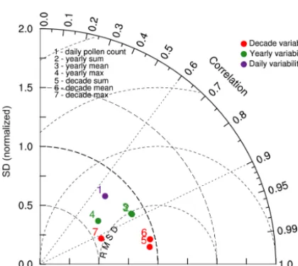
Figure 6. Normalized Taylor diagram showing spatial and temporal

correlations coefficients, standard deviations and RMSEs between simulations and observations for the period 2000–2010. Standard deviation and RMSE are normalized by the standard deviation of observations at the relevant spatiotemporal frequency.

reference OBS, the best is the model skill for this particular variable.

From the diagram, we can see that the model tends to per-form very well when the variability is purely spatial and con-centrations averages over the 11-year period (dots 5, 6 are very close to OBS). Not surprisingly it means the uncertain-ties are reduced to a large extent by the calibration procedure. However, the calibrated simulations do not capture the con-centration maximum as well and tend to underestimate the measured spatial standard deviation (decade maximum dot 7 and also for the annual maximum dot 4). The model does not perform that well, but still shows some realism when the vari-ability is involved in both spatial and temporal correlations. The yearly statistics, which reflect the interannual variation of pollen concentrations over the stations, are captured well with correlation coefficients all above 0.80 and normalized standard deviations of 0.89, 0.88, and 0.61 for concentration

sum, mean, and maximum respectively. When scores are cal-culated for daily concentrations over all the stations, the over-all spatial-temporal correlation coefficient reaches 0.69 for a relative standard deviation of 0.80.

Daily variability is obviously the most difficult to simulate but is at the same time the most relevant in terms of pollen health impact. To investigate this point further, the model per-formance is regionally evaluated with both discrete and cat-egorical statistical indicators as listed in Zhang et al. (2012). The discrete indicators considered in this study include cor-relation coefficient, normalized mean bias factors (NMBF), normalized mean error factors (NMEF), mean fractional bias (MFB), and mean fractional error (MFE). NMBF≤ ±0.25 and NMEF≤0.35 are proposed by Yu et al. (2006) as a cri-teria of good model performance. Boylan and Russell (2006) recommended MFB≤ ±0.30 and MFE≤ ±0.50 as good performance and MFB≤ ±0.60 and MFE≤ ±0.75 as ac-ceptable performance for particulate matter pollution. All metrics are computed over daily time series at each station and on a whole European domain (Table 3). For the whole domain, the average values of NMBF, NMEF, MFB, and MFE are−0.11, 0.83,−0.15, and−0.31, respectively. Ex-cept for NMEF, the indices fall in the range of good per-formance according to the above criteria. The pollen con-centrations over the whole domain are underestimated by a factor of 1.11 based on NMBF. As a measure of absolute gross error, NMEF characterize the spread of the deviation between simulations and observations. Although a relatively large gross error of 0.83 exists, the NMEF obtained here is consistent with what is expected from operational air quality models (Yu et al., 2006; Zhang et al., 2006).

Figure 7. Statistical measures between simulated and observed daily pollen time series for each site: correlation coefficients (a), normalized

mean bias factors (b) and normalized mean error factors (c).

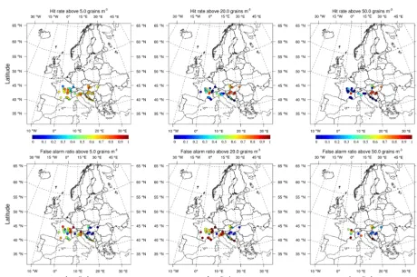
Figure 8. Categorical statistics at thresholds of 5 (left column), 20 (middle column), and 50 grains m−3(right column): upper panel – hit rate (percentage of correctly predicted exceedances to all actual exceedances), lower panel – false alarm ratio (percentage of incorrectly predicted exceedances to all predicted exceedances).

and 79.5 % are within±0.50. In the source regions of cen-tral Europe and eastern France, almost all NMBF values lie within ±0.25. In northern Italy the model mostly over-estimates the mean daily pollen concentrations by factors ranging from 1.25 to above 2.0 (except for ITMAGE sta-tion). Simultaneous overestimation and underestimation can be found for neighbouring stations, which reflects proba-bly the influence of local and patchy sources difficult to ac-count for at 50 km resolution. Better performances are

ob-tained for central European source regions, where the major-ity of NMEF are within 1.0. Performance degrades in France, where most NMEF values are within 1.2. Simulations are more problematic over northern Italy, where values of NMEF are often above 1.2. Generally 51.4 % of the stations with NMEF are within 1.0 and 79.5 % are within 1.4.

Table 3. Model performance on simulation of daily average

con-centrations for 2000–2010.

Discrete statistical indicators

normalized mean bias factors (NMBF) −0.11 normalized mean error factors (NMEF) 0.83 mean fractional bias (MFB) −0.15 mean fractional error (MFE) −0.31 correlation coefficient (R) 0.69

categorical statistical indicators (%) Threshold (grains m−3)

5 20 50

Hit rates 67.9 73.3 74.3

false alarm ratio 33.3 31.9 32.2

exceedances out of all observed exceedances) and false alarm ratio (fraction of incorrectly simulated exceedances out of all simulated exceedances) are calculated from daily time se-ries over the period. On the whole domain, hit rates for these thresholds are 67.9, 73.3, and 74.3 % and false alarm ratios are 33.3, 31.9, and 32.2 %, respectively. The model tends to perform better for high threshold exceedance while giv-ing more false alarms for the lower threshold. As shown on Fig. 8, there are however large regional differences in model performance. Over central European source region, correct prediction often exceed 80 % at moderate and high thresh-olds and false alarms are about 10 % at low and moderate thresholds and 20 % at high threshold. Performance degrades in France and northern Italy source regions, where correct predictions are mostly around 50–70 % at low and moderate thresholds but false alarms are generally high, especially at moderate threshold.

3.4 Ragweed pollen distribution pattern and risk

assessments

With a reasonable confidence in model results, risks region can be identified over the domain. Risk is defined from cer-tain health-relevant concentration thresholds. First we can consider minimum ragweed concentrations triggering an al-lergic reaction. These thresholds are based on experiments involving short exposure time to pollen and then extrapo-lated in order to define health thresholds in terms of daily average concentrations. It is not known, whether a short-time exposure to a large pollen concentration is equivalent to the same dose when less pollen is inhaled over a longer period. Furthermore, these thresholds vary largely between different regions and ethnic groups. The likely range of such daily thresholds is 5–20 grains m−3per day estimated by Oswalt and Marshall (2008). Very sensitive people can be affected by as few as 1–2 pollen grains m−3per day (Bullock et al., 2012).

On this basis, simulated surface concentrations are post-processed to produce 24 h average concentrations. The

foot-Figure 9. Annual footprint of ragweed pollen at the surface,

ob-tained by selecting the maximum from daily averaged concentra-tions during the whole pollen season.

prints of ragweed pollen risk are then obtained by selecting the yearly and monthly maximum from daily averaged con-centrations. The yearly and monthly maximums are averaged over the decade (2000–2010) to produce footprints depicted in Figs. 9, 10). The risk is divided into 16 levels to reflect the range of health relevant threshold used in different countries and regions as listed in Table 4.3 of Bullock et al. (2012). The numbers of grid cells at different threshold risk levels are given in Table 4. Hereafter we select some of the represen-tative risk levels to be discussed in more detail. From annual footprint of ragweed pollen spread risk, the area with con-centration≥1 grains m−3occupies almost 50.3 % area of do-main, with an average concentration of 23.7 grains m−3. The risk pattern extends from European mainland to the seas due to the long-range transport. The lowest risk areas with con-centration of 1–5 grains m−3are located over the sea as well as in the countries upwind and far from the known sources, such as Spain, UK, Poland, Belarus, and Latvia. The low risk areas with concentration of 5–20 grains m−3are found on the periphery of the source regions and over Mediter-ranean Sea, occupying 18.2 % of domain. The intermediate risk areas with concentration of 20–50 grains m−3are close to the sources, taking up 6.1 % of domain. The areas with very strong stress≥50 grains m−3are concentrated on main sources, taking up 5.2 % of domain.

Figure 10. Footprints of ragweed pollen at the surface in each month during pollen season, average from 2000–2010, obtained by selecting

the maximum from daily averaged concentrations in each month.

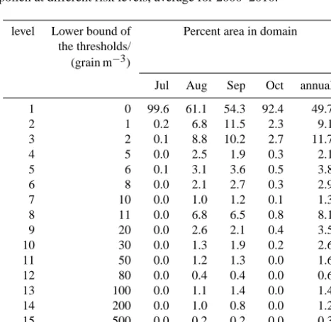
Table 4. Percent area with the surface concentration of ragweed

pollen at different risk levels, average for 2000–2010.

level Lower bound of Percent area in domain the thresholds/

(grain m−3)

Jul Aug Sep Oct annual

1 0 99.6 61.1 54.3 92.4 49.7

2 1 0.2 6.8 11.5 2.3 9.1

3 2 0.1 8.8 10.2 2.7 11.7

4 5 0.0 2.5 1.9 0.3 2.1

5 6 0.1 3.1 3.6 0.5 3.8

6 8 0.0 2.1 2.7 0.3 2.9

7 10 0.0 1.0 1.2 0.1 1.3

8 11 0.0 6.8 6.5 0.8 8.1

9 20 0.0 2.6 2.1 0.4 3.5

10 30 0.0 1.3 1.9 0.2 2.6 11 50 0.0 1.2 1.3 0.0 1.6 12 80 0.0 0.4 0.4 0.0 0.6 13 100 0.0 1.1 1.4 0.0 1.4 14 200 0.0 1.0 0.8 0.0 1.2 15 500 0.0 0.2 0.2 0.0 0.3 16 1000 0.0 0.0 0.0 0.0 0.1

weaker concentrations. The risk areas associated to pollen for each month are given in Table 4.

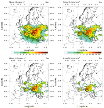
Besides the triggering of allergic reactions at a certain threshold, the time of exposure above a certain threshold might also be important, e.g. in terms of sensitization to rag-weed pollen. To assess a risk based on this criterion, expo-sure time, expressed as the decadal average of the number of days per season above a certain threshold, is calculated and reported in Fig. 11. Relevant thresholds are 5, 10, 20, 50 grain m−3.

Figure 11. Number of days when the daily average concentration exceeding certain risk levels. Ground-based measurement locations are

indicated with circles coloured by the measured number of days (left half) and corresponding simulated number of days (right half).

4 Summary and conclusions

This study presents a regional-climatic simulation frame-work based on RegCM4 for investigating the dynamics of emissions and transport of ragweed pollen. The RegCM-pollen modelling system incorporates a RegCM-pollen emission module coupled to CLM4.5 and a transport module as part of the chemistry transport component of RegCM. Because cli-mate, CLM4.5 and chemistry components are synchronously coupled to the RegCM model, this approach allows dynam-ical response of pollen ripening, release, and dispersion to key environmental drivers like temperature, photoperiod, soil moisture, precipitation, relative humidity, turbulence, and wind. Through the pollen production link to NPP, other en-vironmental and climate relevant factors as atmospheric CO2 concentrations are also accounted for. The specific ragweed phenology is parameterized from growth controlled exper-iment but has to be somehow adjusted to observations for more realism of the flowering season simulations over Eu-rope. Similarly, ragweed spatial distribution is a very poorly constrained parameter which has to be corrected through a

calibration procedure. The calibration is performed consid-ering the decadal mean of pollen counts over all sites. As a result the spatial correlation between the simulated and measured average concentrations over the decade is greatly increased (from 0.23 to 0.98) by the calibration. While the cross validation aimed at evaluating the calibration shows a corresponding correlation of 0.54 and RESM of 21 %, which reflects reasonable error and sensitivity of the calibration. The model measurement correlations based on daily com-parison, which are the most relevant for pollen impacts also increase from 0.28 to 0.69. The simulation of daily and in-terannual variability of pollen concentrations reflect model skills that do not purely rely on the calibration since this one is performed on decadal mean of yearly pollen count.

source regions are reproduced fairly well while in the ar-eas with lower ragweed infestation the deviations are evi-dent. The model in general captures the gross features of the pollen concentrations found in Europe. Statistical measures of NMBF, MFB, and MFE over the domain fall in the range of recommendation for a good performance while NMEF is a bit large with a value of 0.83. The model performs bet-ter over the central European source region, where the daily correlations at most stations are above 0.6–0.7 and NMEF lie within 1.0. Performance tends to degrade in France and northern Italy. Still, the values of NMEF for pollen simula-tion are generally consistent with what is expected from op-erational air quality models for aerosols for example. Cate-gorical evaluation reveals the model tends to give better pre-dictions for high threshold while giving more false alarms for low threshold. A better performance is also shown over the central European source region at all levels, with correct predictions above 80 % and false alarms within 20 %.

The multi-annual average footprints of ragweed pollen spread risk are produced from calibration simulations. The pollen plume with concentration ≥1 grains m−3 can reach seas far away from the European mainland. The risk areas with concentration above 5 grains m−3are around the source and on Mediterranean Sea, occupying a total of 29.5 % of domain. While the areas with very strong stress ≥50 grains m−3 are confined in narrow source areas. From the seasonal distribution, August in general contributes most to the annual footprint and September shows important levels. The longest risk exposure time occurs on Pannonian Plain at all thresholds. Northern Italy and France also show some considerable exposure times.

The modelling framework presented here allows simulta-neous estimation of ragweed pollen risk both for hindcast simulations (including sensitivity studies to different param-eters) and for study of potential risk evolution changes under future climate scenarios as illustrated in Hamaoui-Laguel et al. (2015). Still a long list of uncertainties hinders an accu-rate estimate of the airborne pollen patterns and risk within the presented framework. Caution should also be taken while interpreting the results in areas without a dense observational network and where calibration is weaker. In this regard, chal-lenging research efforts should focus on a better characteri-zation of ragweed spatial distributions and biomass, in ad-dition, a better understanding of phenological process and the dynamic response of release rate to meteorological con-ditions will help to reduce these uncertainties and improve model performance. An accurate and diverse observation of ragweed phenology is therefore essential to better represent local flowering and there is also a need for experimental ob-servations to better constrain the release model. In parallel, systematic ragweed pollen concentrations should be further developed as part of air quality networks and public access to data should be promoted.

Data availability

CRUNCEP atmospheric forcing data are available at http://dods.extra.cea.fr/store/p529viov/cruncep/ V5_1901_2013. Data description is available at http://dods.extra.cea.fr/data/p529viov/cruncep/readme.htm.

Acknowledgements. This research is funded by the European

Union’s Seventh Framework Programme (FP7/2007–2013) under grant agreements no. 282687 Atopica (http://cordis.europa.eu/fp7). We thank the contributors of ragweed distribution data. Pollen observation data are kindly provided by the European Aeroaller-gen Network, Reseau National de Surveillance Aerobiologique, ARPA-Veneto, ARPA-FVG, Croatian Institute of Public Health, the Department of Environmental Protection and Health Ecology at Institute of Public Health “Andrija Štampar” and Associate-degree college of Velika Gorica. Constructive comments from two anony-mous reviewers improved the quality of this paper a lot.

Edited by: S. Fontaine

References

Allard, H. A.: Flowering behaviour and natural distribution of the eastern ragweeds (Ambrosia) as affected by length of day, Ecol-ogy, 26, 387–394, 1945.

Boylan, J. W. and Russell, A. G.: PM and light extinction model performance metrics, goals, and criteria for three-dimensional air quality models, Atmos. Environ., 40, 4946–4959, 2006. Bullock, J. M., Chapman, D., Schafer, S., Roy, D., Girardello,

M., Haynes, T., Beal, S., Wheeler, B., Dickie, I., Phang, Z., Tinch, R., ˇCivi´c, K., Delbaere, B., Jones-Walters, L., Hilbert, A., Schrauwen, A., Prank, M., Sofiev, M., Niemelä, S., Räisänen, P., Lees, B., Skinner, M., Finch, S., and Brough, C.: Assessing and controlling the spread and the effects of common ragweed in Europe, Final Report ENV.B2/ETU/2010/0037, European Com-mission, 456 pp., 2012.

Burbach, G. J., Heinzerling, L. M., Röhnelt, C., Bergmann, K.-C., Behrendt, H., and Zuberbier, T.: Ragweed sensitization in Europe – GA(1)LEN study suggests increasing prevalence, Allergy, 64, 664–665, 2009.

Cecchi, L., Morabito, M., Domeneghetti, M. P., Crisci, A., Ono-rari, M., and Orlandini, S.: Long distance transport of ragweed pollen as a potential cause of allergy in central Italy, Ann. Al-lerg. Asthma. Im., 96, 86–91, 2006.

Chapman, D. S., Haynes, T., Beal, S., Essl, F., and Bullock, J. M.: Phenology predicts the native and invasive range limits of com-mon ragweed, Glob. Change Biol., 20, 192–202, 2014.

Chauvel, B., Dessaint, F., Cardinal-Legrand, C., and Bretagnolle, F.: The historical spread of Ambrosia artemisiifolia L. in France from herbarium records, J. Biogeogr., 33, 665–673, 2006. Dahl, A., Strandhede, S.-O., and Wihl, J.-A.: Ragweed – An allergy

risk in Sweden?, Aerobiologia, 15, 293–297, 1999.

Deen, W., Hunt, L. A., and Swanton, C. J.: Photothermal time de-scribes common ragweed (Ambrosia artemisiifolia L.) phenolog-ical development and growth, Weed Sci., 46, 561–568, 1998a. Deen, W., Hunt, T., and Swanton, C. J.: Influence of temperature,

photoperiod, and irradiance on the phenological development of common ragweed (Ambrosia artemisiifolia), Weed Sci., 46, 555– 560, 1998b.

Deen, W., Swanton, C. J., and Hunt, L. A.: A mechanistic growth and development model of common ragweed, Weed Sci., 49, 723–731, 2001.

Efstathiou, C., Isukapalli, S., and Georgopoulos, P.: A mechanistic modeling system for estimating large-scale emissions and trans-port of pollen and co-allergens, Atmos. Environ., 45, 2260–2276, 2011.

Emanuel, K. A. and Zivkovic-Rothman, M.: Development and eval-uation of a convection scheme for use in climate models, J. At-mos. Sci., 56, 1766–1782, 1999.

Fumanal, B., Chauvel, B., and Bretagnolle, F.: Estimation of pollen and seed production of common ragweed in France, Ann. Agr. Env. Med., 14, 233–236, 2007.

Galán, C., Smith, M., Thibaudon, M., Frenguelli, G., Oteros, J., Gehrig, R., Berger, U., Clot, B., and Brandao, R.: Pollen mon-itoring: minimum requirements and reproducibility of analysis, Aerobiologia, 30, 385–395, 2014.

Gallinza, N., Bari´c, K., Š´cepanovi´c, M., Gorši´c, M., and Ostoji´c, Z.: Distribution of invasive weed Ambrosia artemisiifolia L. in Croatia, Agriculturae Conspectus Scientificus, 75, 75–81, 2010. García-Mozo, H., Galán, C., Belmonte, J., Bermejo, D., Candau,

P., Díaz de la Guardia, C., Elvira, B., Gutiérrez, M., Jato, V., Silva, I., Trigo, M. M., Valencia, R., and Chuine, I.: Predicting the start and peak dates of the Poaceae pollen season in Spain using process-based models, Agr. Forest Meteorol., 149, 256– 262, 2009.

Giorgi, F., Pal, J. S., Bi, X., Sloan, L., Elguindi, N., and Solmon, F.: Introduction to the TAC special issue: The RegCNET network, Theor. Appl. Climatol., 86, 1–4, doi:10.1007/s00704-005-0199-z, 2006.

Giorgi, F., Coppola, E., Solmon, F., Mariotti, L., Sylla, M. B., Bi, X., Elguindi, N., Diro, G. T., Nair, V., Giuliani, G., Turuncoglu, U. U., Cozzini, S., Güttler, I., O’Brien, T. A., Tawfik, A. B., Shalaby, A., Zakey, A. S., Steiner, A. L., Stordal, F., Sloan, L. C., and Brankovic, C.: RegCM4: model description and preliminary tests over multiple CORDEX domains, Clim. Res., 52, 7–29, 2012. Grell, G. A.: Prognostic Evaluation of Assumptions Used by

Cumu-lus Parameterizations, Mon. Weather Rev., 121, 764–787, 1993. Guenther, A. B., Jiang, X., Heald, C. L., Sakulyanontvittaya, T.,

Duhl, T., Emmons, L. K., and Wang, X.: The Model of Emissions of Gases and Aerosols from Nature version 2.1 (MEGAN2.1): an extended and updated framework for modeling biogenic emis-sions, Geosci. Model Dev., 5, 1471–1492, 2012.

Hamaoui-Laguel, L., Vautard, R., Liu, L., Solmon, F., Viovy, N., Khvorostyanov, D., Essl, F., Chuine, I., Colette, A., Semenov, M. A., Schaffhauser, A., Storkey, J., Thibaudon, M., and Epstein, M. M.: Effects of climate change and seed dispersal on airborne ragweed pollen loads in Europe, Nature Climate Change, 5, 766– 771, 2015.

Helbig, N., Vogel, B., Vogel, H., and Fiedler, F.: Numerical mod-elling of pollen dispersion on the regional scale, Aerobiologia, 20, 3–19, 2004.

Hirst, J. M.: An Automatic Volumetric Spore Trap, Ann. Appl. Biol., 39, 257–265, 1952.

Holtslag, A. A. M., De Bruijn, E. I. F., and Pan, H.-L.: A high-resolution air-mass transformation model for short-range weather forecasting, Mon. Weather Rev., 118, 1561–1575, 1990. Hurtt, G. C., Frolking, S., Fearon, M. G., Moore, B., Shevliakova, E., Malyshev, S., Pacala, S. W., and Houghton, R. A.: The un-derpinnings of land-use history: three centuries of global grid-ded land-use transitions, wood-harvest activity, and resulting sec-ondary lands, Glob. Change Biol., 12, 1208–1229, 2006. Jäger, S., Mandroli, P., Spieksma, F., Emberlin, J., Hjelmroos, M.,

Rantio-Lehtimaki, A., and Al, E.: News, Aerobiologia, 11, 69– 70, 1995.

Jato, V., Rodriguez-Rajo, F. J., Alcázar, P., De Nuntiis, P., Galán, C., and Mandrioli, P.: May the definition of pollen season influence aerobiological results?, Aerobiologia, 22, 13–25, 2006. Karrer, G., Skjøth, C. A., Šikoparija, B., Smith, M., Berger, U., and

Essl, F.: Ragweed (Ambrosia) pollen source inventory for Aus-tria, Sci. Total Environ., 523, 120–128, 2015.

Kazinczi, G., Béres, I., Pathy, Z., and Novák, R.: Common ragweed (Ambrosia artemisiifolia L.): a review with special regards to the results in Hungary: II. Importance and harmful effect, allergy, habitat, allelopathy and beneficial characteristics, Herbologia, 9, 93–117, 2008.

Martin, M. D., Chamecki, M., and Brush, G. S.: Anthesis synchro-nization and floral morphology determine diurnal patterns of rag-weed pollen dispersal, Agr. Forest Meteorol., 150, 1307–1317, 2010.

Meleux, F., Solmon, F., and Giorgi, F.: Increase in summer Euro-pean ozone amounts due to climate change, Atmos. Environ., 41, 7577–7587, 2007.

Oleson, K. W., Lawrence, D. M., Bonan, G. B., Drewniak, B., Huang, M., Koven, C. D., Levis, S., Li, F., Riley, W. J., Subin, Z. M., Swenson, S. C., Thornton, P. E., Bozbiyik, A., Fisher, R., Heald, C. L., Kluzek, E., Lamarque, J.-F., Lawrence, P. J., Le-ung, L. R., Lipscomb, W., Muszala, S., Ricciuto, D. M., Sacks, W., Sun, Y., Tang, J., and Yang, Z.-L.: Technical description of version 4.5 of the Community Land Model (CLM), NCAR Technical Note NCAR/TN-503+STR, National Center for At-mospheric Research, Boulder, Colorado, 434 pp., 2013. Oswalt, M. L. and Marshall, G. D.: Ragweed as an example of

worldwide allergen expansion, Allergy Asthma Clin. Immunol., 4, 130–135, 2008.

Pal, J. S., Small, E. E., and Eltahir, E. A. B.: Simulation of regional-scale water and energy budgets: Representation of subgrid cloud and precipitation processes within RegCM, J. Geophys. Res. At-mos., 105, 29579–29594, 2000.

Pal, J. S., Giorgi, F., Bi, X., Elguindi, N., Solmon, F., Rauscher, S. A., Gao, X., Francisco, R., Zakey, A., Winter, J., Ashfaq, M., Syed, F. S., Sloan, L. C., Bell, J. L., Diffenbaugh, N. S., Karma-charya, J., Konaré, A., Martinez, D., da Rocha, R. P., and Steiner, A. L.: Regional climate modeling for the developing world: the ICTP RegCM3 and RegCNET, B. Am. Meteorol. Soc., 88, 1395– 1409, 2007.

Payne, W. W.: The morphology of the inflorescence of ragweeds (Ambrosia-Franseria: Compositae), Am. J. Bot., 50, 872–880, 1963.

Am-brosia artemisiifolia in arable fields in Hungary, Preslia, 83, 219– 235, 2011.

Prank, M., Chapman, D. S., Bullock, J. M., Belmonte, J., Berger, U., Dahl, A., Jager, S., Kovtunenko, I., Magyar, D., Niemela, S., Rantio-Lehtimaki, A., Rodinkova, V., Sauliene, I., Severova, E., Sikoparija, B., and Sofiev, M.: An operational model for forecast-ing ragweed pollen release and dispersion in Europe, Agr. Forest Meteorol., 182, 43–53, 2013.

Rogers, C. A., Wayne, P. M., Macklin, E. A., Muilenberg, M. L., Wagner, C. J., Epstein, P. R., and Bazzaz, F. A.: Interaction of the onset of spring and elevated atmospheric CO2on ragweed (Ambrosia artemisiifolia L.) pollen production, Environ. Health Persp., 114, 865–869, 2006.

Shalaby, A. K., Zakey, A. S., Tawfik, A. B., Solmon, F., Giorgi, F., Stordal, F., Sillman, S., Zaveri, R. A., and Steiner, A. L.: Imple-mentation and evaluation of online gas-phase chemistry within a regional climate model (RegCM-CHEM4), Geosci. Model Dev., 5, 741–760, doi:10.5194/gmd-5-741-2012, 2012.

Shrestha, A., Roman, E. S., Thomas, A. G., and Swanton, C. J.: Modeling germination and shoot-radicle elongation of Ambrosia artemisiifolia, Weed Sci., 47, 557–562, 1999.

Šikoparija, B., Skjøth, C. A., Radiši´c, P., Stjepanivi´c, B., Hrga, I., Apatini, D., Martinez, D., Páldy, A., Ianovici, N., and Smith, M.: Aerobiology data used for producing inventories of inva-sive species, in: Proceedings of the international symposium on current trends in plant protection, Belgrade, Serbi, 8 September 2012, 7–14, 2012.

Šikoparija, B., Skjøth, C. A., Kübler, K. A., Dahl, A., Sommer, J., Grewling, Ł., Radiši´c, P., and Smith, M.: A mechanism for long distance transport of Ambrosia pollen from the Pannonian Plain, Agr. Forest Meteorol., 180, 112–117, 2013.

Simard, M. J. and Benoit, D. L.: Effect of repetitive mowing on common ragweed (Ambrosia Artemisiifolia L.) pollen and seed production, Ann. Agr. Env. Med., 18, 55–62, 2011.

Simard, M. J. and Benoit, D. L.: Potential pollen and seed produc-tion from early- and late-emerging common ragweed in corn and soybean, Weed Technol., 26, 510–516, 2012.

Skjøth, C. A.: Integrating measurements, phenological models and atmospheric models in aerobiology, Ph.D. thesis, Copenhagen University and National Environmental Research Institute, Den-mark, 123 pp., 2009.

Skjøth, C. A., Smith, M., Šikoparija, B., Stach, A., Myszkowska, D., Kasprzykf, I., Radiši´c, P., Stjepanovi´c, B., Hrga, I., Apatini, D., Magyar, D., Páldy, A., and Ianovici, N.: A method for produc-ing airborne pollen source inventories: An example of Ambrosia (ragweed) on the Pannonian Plain, Agr. Forest Meteorol., 150, 1203–1210, 2010.

Smith, M., Skjøth, C. A., Myszkowska, D., Uruska, A., Puc, M., Stach, A., Balwierz, Z., Chlopek, K., Piotrowska, K., Kasprzyk, I., and Brandt, J.: Long-range transport of Ambrosia pollen to Poland, Agr. Forest Meteorol., 148, 1402–1411, 2008.

Smith, M., Cecchi, L., Skjøth, C. A., Karrer, G., and Šikoparija, B.: Common ragweed: A threat to environmental health in Europe, Environ. Int., 61, 115–126, 2013.

Sofiev, M., Siljamo, P., Ranta, H., and Rantio-Lehtimäki, A.: To-wards numerical forecasting of long-range air transport of birch pollen: theoretical considerations and a feasibility study, Int. J. Biometeorol., 50, 392–402, 2006.

Sofiev, M., Siljamo, P., Ranta, H., Linkosalo, T., Jaeger, S., Ras-mussen, A., Rantio-Lehtimaki, A., Severova, E., and Kukkonen, J.: A numerical model of birch pollen emission and dispersion in the atmosphere, Description of the emission module, Int. J. Biometeorol., 57, 45–58, 2013.

Sofiev, M., Berger, U., Prank, M., Vira, J., Arteta, J., Belmonte, J., Bergmann, K. C., Chéroux, F., Elbern, H., Friese, E., Galan, C., Gehrig, R., Khvorostyanov, D., Kranenburg, R., Kumar, U., Marécal, V., Meleux, F., Menut, L., Pessi, A. M., Robertson, L., Ritenberga, O., Rodinkova, V., Saarto, A., Segers, A., Severova, E., Sauliene, I., Siljamo, P., Steensen, B. M., Teinemaa, E., Thibaudon, M., and Peuch, V. H.: MACC regional multi-model ensemble simulations of birch pollen dispersion in Europe, At-mos. Chem. Phys., 15, 8115–8130, 10.5194/acp-15-8115-2015, 2015.

Solmon, F., Giorgi, F., and Liousse, C.: Aerosol modelling for re-gional climate studies: application to anthropogenic particles and evaluation over a European/African domain, Tellus B, 58, 51–72, 2006.

Solmon, F., Elguindi, N., and Mallet, M.: Radiative and climatic ef-fects of dust over West Africa, as simulated by a regional climate model, Clim. Res., 52, 97–113, 2012.

Stach, A., Smith, M., Skjøth, C. A., and Brandt, J.: Examining Am-brosia pollen episodes at Poznan (Poland) using back-trajectory analysis, Int. J. Biometeorol., 51, 275–286, 2007.

Storkey, J., Stratonovitch, P., Chapman, D. S., Vidotto, F., and Semenov, M. A.: A process-based approach to predict-ing the effect of climate change on the distribution of an invasive allergenic plant in Europe, Plos One, 9, e88156, doi:10.1371/journal.pone.0088156, 2014.

Taramarcaz, P., Lambelet, C., Clot, B., Keimer, C., and Hauser, C.: Ragweed (Ambrosia) progression and its health risks: will Switzerland resist this invasion?, Swiss Med. Wkly., 135, 538– 548, 2005.

Thibaudon, M., Šikoparija, B., Oliver, G., Smith, M., and Skjøth, C. A.: Ragweed pollen source inventory for France – The second largest centre of Ambrosia in Europe, Atmos. Environ., 83, 62– 71, 2014.

Thornton, P. E., Law, B. E., Gholz, H. L., Clark, K. L., Falge, E., Ellsworth, D. S., Golstein, A. H., Monson, R. K., Hollinger, D., Falk, M., Chen, J., and Sparks, J. P.: Modeling and measuring the effects of disturbance history and climate on carbon and water budgets in evergreen needleleaf forests, Agr. Forest Meteorol., 113, 185–222, 2002.

Thornton, P. E., Lamarque, J. F., Rosenbloom, N. A., and Mahowald, N. M.: Influence of carbon-nitrogen cycle cou-pling on land model response to CO2 fertilization and climate variability, Global Biogeochem. Cy., 21, GB4018, doi:10.1029/2006gb002868, 2007.

Tummon, F., Solmon, F., Liousse, C., and Tadross, M.: Simulation of the direct and semidirect aerosol effects on the southern Africa regional climate during the biomass burning season, J. Geophys. Res.-Atmos., 115, D19206, doi:10.1029/2009JD013738, 2010. Viovy, N.: CRUNCEP dataset, Description available at:

http://dods.extra.cea.fr/data/p529viov/cruncep/readme.htm, Data available at: http://dods.extra.cea.fr/store/p529viov/ cruncep/V5_1901_2013, 2011.

dormancy in common ragweed seeds, Am. J. Bot., 62, 1–5, doi:10.2307/2442073, 1975.

Yu, S. C., Eder, B., Dennis, R., Chu, S.-H., and Schwartz, S. E.: New unbiased symmetric metrics for evaluation of air quality models, Atmos. Sci. Lett., 7, 26–34, 2006.

Zakey, A. S., Solmon, F., and Giorgi, F.: Implementation and test-ing of a desert dust module in a regional climate model, At-mos. Chem. Phys., 6, 4687–4704, doi:10.5194/acp-6-4687-2006, 2006.

Zhang, R., Duhl, T., Salam, M. T., House, J. M., Flagan, R. C., Avol, E. L., Gilliland, F. D., Guenther, A., Chung, S. H., Lamb, B. K., and VanReken, T. M.: Development of a regional-scale pollen emission and transport modeling framework for investi-gating the impact of climate change on allergic airway disease, Biogeosciences, 11, 1461–1478, doi:10.5194/bg-11-1461-2014, 2014.

Zhang, Y., Liu, P., Queen, A., Misenis, C., Pun, B., Seigneur, C., and Wu, S.-Y.: A comprehensive performance evaluation of MM5-CMAQ for the Summer 1999 Southern Oxidants Study episode – Part II: Gas and aerosol predictions, Atmos. Environ., 40, 4839– 4855, 2006.

Zhang, Y., Bocquet, M., Mallet, V., Seigneur, C., and Baklanov, A.: Real-time air quality forecasting, Part I: History, techniques, and current status, Atmos. Environ., 60, 632–655, 2012.

Zink, K., Vogel, H., Vogel, B., Magyar, D., and Kottmeier, C.: Mod-eling the dispersion of Ambrosia artemisiifolia L. pollen with the model system COSMO-ART, Int. J. Biometeorol., 56, 669–680, 2012.