www.ann-geophys.net/29/1571/2011/ doi:10.5194/angeo-29-1571-2011
© Author(s) 2011. CC Attribution 3.0 License.
Annales
Geophysicae
The proton pressure tensor as a new proxy of the proton decoupling
region in collisionless magnetic reconnection
N. Aunai1, A. Retin`o1, G. Belmont1, R. Smets1, B. Lavraud2,3, and A. Vaivads4
1Laboratoire de Physique des Plasmas, UMR 7648, Ecole Polytechnique, Route de Saclay, 91128 Palaiseau, France 2Institut de Recherche en Astrophysique et Plan´etologie, Universit´e de Toulouse (UPS), France
3Centre National de la Recherche Scientifique, UMR 5277, Toulouse, France 4Swedish Institute of Space Physics, P.O. Box 537, 75121 Uppsala, Sweden
Received: 1 July 2011 – Revised: 31 August 2011 – Accepted: 5 September 2011 – Published: 12 September 2011
Abstract. Cluster data is analyzed to test the proton pressure tensor variations as a proxy of the proton decoupling region in collisionless magnetic reconnection. The Hall electric po-tential well created in the proton decoupling region results in bounce trajectories of the protons which appears as a charac-teristic variation of one of the in-plane off-diagonal compo-nents of the proton pressure tensor in this region. The event studied in this paper is found to be consistent with classical Hall field signatures with a possible 20 % guide field. More-over, correlations between this pressure tensor component, magnetic field and bulk flow are proposed and validated, to-gether with the expected counterstreaming proton distribu-tion funcdistribu-tions.
Keywords. Space plasma physics (Magnetic reconnection)
1 Introduction
Magnetic reconnection is an important plasma phenomenon transferring the magnetic energy stored in current sheets into fluid kinetic energy and heat and allowing the breaking of the large scale flux freezing constraint. It has important conse-quences regarding the dynamics of many astrophysical envi-ronments like the Earth’s magnetosphere and its interaction with the solar wind (Dungey, 1961; Priest and Forbes, 2000; Birn and Priest, 2007; Yamada et al., 2010).
One of the most remarkable consequences of magnetic re-connection is the formation of plasma jets. In collisionless environments, these jets are formed within a microscopic re-gion surrounding the reconnection site, called the ion decou-pling region. When the scale of the current sheet reaches the ion inertial scale, the ion fluid (hereafter considered to be a proton fluid) cannot follow the magnetic field motion
Correspondence to: N. Aunai (nicolas.aunai@lpp.polytechnique.fr)
and decouples from it. At this scale, the latter is therefore only frozen in the electron fluid, which, because it is much lighter, can move very much faster. The decoupling of the protons enables Hall electric fields which in return acceler-ate them away from the reconnection site up to a large frac-tion of the upstream Alfv´en speed within a few proton in-ertial lengths. This mechanism self-consistently adjusts the reconnection geometry and therefore the rate at which the phenomenon proceeds (Birn et al., 2001).
The proton decoupling region is so small compared to the magnetosphere characteristic scale that it is rarely crossed in spite of the increasing number of space probes. When it is crossed, the highly dynamic and multiscale behavior of plasma structures makes the analysis so difficult that we only begin to gather enough evidences for just being con-vinced that reconnection is indeed happening and seem to be consistent with the numerical models (Paschmann, 2008). Among these evidences are the repeated observations of elec-tromagnetic and bulk flow correlations consistent with the classic two-dimensional Hall model (Eastwood et al., 2010a). As uncertainties on the physical interpretation of spacecraft measurements are today almost impossible to evaluate, a de-tailed study of the collisionless reconnection mechanism it-self by observational means is still very challenging and quires as much observational proxies of the critical Hall re-gion as possible.
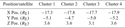
Table 1. Position of Cluster spacecraft in the GSM coordinate
sys-tem at 17:00 UT.
Position/satellite Cluster 1 Cluster 2 Cluster 3 Cluster 4
X Pos. (RE) −17.3 −17.8 −17.7 −17.9
Y Pos. (RE) −5.1 −4.7 −5.0 −5.2
Z Pos. (RE) 3.6 3.6 3.1 3.6
protons bouncing in the electrostatic potential well. Sim-ilar beams were also observed in kinetic numerical simu-lations and sometimes interpreted as well as the result of bounce trajectories of the protons between the separatrices in the decoupling region (Pei et al., 2001; Shay et al., 1998). It is worth noticing, however, that counterstreaming beams seem to be a common feature in space plasma observations and may appear in different contexts in numerical simula-tions as well (Nagai et al., 2001; Drake et al., 2009; Gosling et al., 2005). Recently, an analysis of the proton accelera-tion within the decoupling region, from both fluid and ki-netic point of views, using two-dimensional hybrid simula-tions confirmed the scenario of Wygant et al. (2005): pro-tons bounce in the Hall electrostatic potential well, create counterstreaming beam distributions that effectively increase the pressure inside the exhaust and balance the normal in-ward electric force (Aunai et al., 2011a,b). Their analysis went a step beyond and can be summarized in the following way: they revealed that the outflow directed component of the Hall electric force (enEx), was also partly balanced by a
pressure force, also linked to the kinetic bounce mechanism. They showed that as the protons bounce between the separa-trices, the small aperture angle of the electrostatic potential well makes them to deviate at each bounce and transfer the velocity gained from the potential, from the normal (z) to the outflow direction (x). At a fixed position within the exhaust region, the collisionless mixing of protons having bounced a different number of times thus statistically couples the nor-mal and outflow velocity component of particle velocity in phase space, which macroscopically appears as non-zero in-plane off-diagonal component of the proton pressure tensor (PN Lin LMN coordinates).
They also showed that as the strong Hall electric field dis-appears as one moves away from the decoupling region in the downstream direction, the bounce mechanism ceases and the spatial structure of the in-plane off-diagonal component of the pressure tensor changes. These results, beyond the study of the fundamental acceleration mechanism, therefore suggest the spatial structure of this component of the proton pressure tensor as an additional observational proxy of the proton decoupling region.
The present paper investigates, by means of spacecraft data analysis, the proton acceleration in the vicinity of the decoupling (Hall) region and focuses on the relationship be-tween the bounce mechanism and the fluid consequences via
tured as follows. The second section presents the dataset in terms of spacecraft orbit, tetrahedron configuration and in-struments used. The third section presents an overview of the electromagnetic and proton moments during the time in-terval of interest. In the fourth section, we show the study of the “classical” correlations of the magnetic field and the proton bulk flow and compare it to the classical 2-D Hall re-connection scenario. Deducing roughly the spatial structure from the previous analysis, we present in the fifth section, theoretical predictions for the correlation of the in-plane off-diagonal component of the proton pressure tensor with the electromagnetic field and bulk flow based on previous sim-ulation results (Aunai et al., 2011a,b), and confront it with observations. In the sixth section, we present the in-plane projection of the measured proton distribution functions in specific regions where we expect to see beams consistent with the bounce proton motion in the open potential well. The last section summarizes our results and discusses future work.
2 Dataset and orbit
This study focuses on the data measured by the Cluster spacecraft (Escoubet et al., 2001) during the time interval 17:05–17:35 UT, on 18 August 2002. At this time, the four satellites are located near the magnetotail current sheet. The tetrahedron configuration is given in the Fig. 1 and the po-sition of the satellites at the time of the event is reported in Table 1. In this study, we have used the data measured by the Flux-Gate Magnetometer (FGM) experiment (Balogh et al., 2001) with full resolution. The proton moments were mea-sured by Cluster Ion Spectrometry (CIS) experiment (R`eme et al., 2001) with the CODIF instrument, and proton distri-bution functions were measured by the HIA instrument, both with spin (4 s) resolution. The electric field and spacecraft potential were measured by the Electric Field and Waves (EFW) instrument (Gustafsson et al., 2001).
3 Event overview
Figure 2 summarizes some of the data measured by Clus-ter 1 and 4 spacecraft during the time inClus-terval of inClus-terest. The magnetic field (Bx,By,Bz), proton bulk flow (Vx) and proton
pressure tensor component (Pxz) are presented in panels (c),
Fig. 1. Tetrahedron configuration in the GSM coordinate system for August 18th 2002 between 15:00:00 and 18:00:00 U.T. Red circles indicate the configuration at 17:00:00, approximate time of the event. Black, Red, Green and Blue indicate Cluster1,2,3and4, respectively.
Position/Satellite Cluster1 Cluster2 Cluster3 Cluster4 X Pos. (RE) −17.3 −17.8 −17.7 −17.9 Y Pos. (RE) −5.1 −4.7 −5.0 −5.2 Z Pos. (RE) 3.6 3.6 3.1 3.6
Table 1. Position of Cluster spacecraft in the GSM coordinate system at 17:00 U.T.
4
Fig. 1. Tetrahedron configuration in the GSM coordinate system
for 18 August 2002 between 15:00:00 and 18:00:00 UT. Red cir-cles indicate the configuration at 17:00:00, approximate time of the event. Black, Red, Green and Blue indicate Cluster 1, 2, 3 and 4, respectively.
electron physics point of view ( ˚Asnes et al., 2008). The mag-netic reversal seen aroundt=17:07:40, followed by the bulk flow reversal in the x-direction aroundt=17:08:40 are in-teresting features when considering magnetic reconnection. Also consistent with the reconnection scenario is the reversal of theBz magnetic component. When combined together,
these features might indicate that the spacecraft crossed a re-connection region from its northern tailward side to its south-ern earthward side (cf. Fig. 3). Two flow reversals are also measured afterwards and might indicate the crossing of the same fluctuating X-line or the crossing of other X-lines. It is worth noticing that in the mean time,C1andC4measured
variations of theBycomponent of the magnetic field
corre-lated with the bulk flow reversals, as expected for a crossing of the proton decoupling region from the 2-D Hall recon-nection model where the reconrecon-nection would happen in the (x,z) plane. We will analyze in detail the variations of the magnetic and velocity field and compare it to theoretical pre-dictions in Sect. 4.
Figure 2g presents the variations of thePxzcomponent of
the proton pressure tensor. Let us note for the moment that first, it is not zero, indicating an anisotropy of the distribu-tion funcdistribu-tion of the protons. Then it shows variadistribu-tions and changes sign in correlation with the flow and magnetic mea-surements. These variations and their correlation with the other quantities will be discussed in detail in Sect. 5.
(nT)
(nT)
(km/s)
(nPa) C
D
E
F
G (nT) (cm )-3
(mV)
(mV/m) A
[image:3.595.47.290.60.304.2]B
Fig. 2. Overview of the data measured by Cluster 1 and 4 spacecraft
on 18 August 2002. Vectors are presented in the GSM coordinate system.
Figure 2a presents the proton density and the spacecraft potential measured by Cluster 1. One can notice that the pro-ton density calculated from the particle instrument is con-sistent with the variations of the spacecraft potential. The presence of density and potential dips in the signal at about 17:07:00, 17:08:00 and 17:09:00 will be discussed as possi-ble proxies for the reconnection region structure.
Finally, Fig. 2b presents the electric field in the z-direction of the DeSpun Inverted (DSI) coordinate system measured byC4. This component is calculated using the E·B=0
[image:3.595.312.545.62.490.2]Table 2. LMN basis for Cluster 1 (L1M1N1) and Cluster 4
(L4M4N4) in GSE coordinates.
x y z
L1 0.9708 0.2362 −0.0417
M1 −0.2487 0.9286 0.2754
N1 0.1006 −0.2668 0.9585
L4 0.9949 0.0645 −0.0774
M4 −0.1769 0.9107 0.3731
N4 0.1142 −0.4131 0.9034
4 Proton decoupling region: Hall signatures
4.1 LMN coordinate system
The data overview presented in Fig. 2 shows variations in theBycomponent, correlated with those of the bulk flow and
magnetic field in the x-direction. In this section, we ana-lyze more closely these correlations and compare it to what is expected from the two-dimensional collisionless reconnec-tion model. Assuming the reconnecreconnec-tion process to be pla-nar, we first need to identify the appropriate basis to project vectors and compare them with classical Hall reconnection model. When crossing a reconnection outflow region, one can usually distinguish the variation scales of the three mag-netic components. The largest variation is attributed to the reconnecting component, which in the magnetotail is usu-ally close to the x-direction. The intermediate variation is attributed to the Hall magnetic component, which points in the out-of-plane direction (usually the y-direction in the tail). And finally the negligible variation is attributed to the normal component (close to z-direction). We performed a minimum variance analysis (MVA) centered on theBxreversal time to
determine these largest, intermediate and smallest variation directions and found, for each spacecraft, the corresponding LMN vectors, for which the GSE components are given in Table 2. Both matrices are roughly similar to the GSM coor-dinate system. In the following, the LMN coorcoor-dinate system is used to perform and present our analysis since the vari-ous features a more consistent with the reconnection scenario when the data is projected in this basis.
4.2 Evidences for a small guide field
Looking carefully at the data overview presented in Fig. 2, one can note that theBy component is not zero when Bx
changes its sign. Because the Hall magnetic component is quadrupolar around the reconnection site, this might indicate the presence of a small guide field, whose value would then be precisely theByvalue whenBx=0, that isBGF≈4 nT.
This suggestion is consistent with the fact that By is also
about 4 nT at the bulk flow reversal (Fig. 2). Figure 3 rep-resents scatter plots of theBM component of the magnetic
(BL,VL) C1 C4
and 17:09:45. For each spacecraft, we have also represented a scatter plot ofBM0 in the same plane, defined asBM−BGF.
Each scatter plot is accompanied by a cartoon, illustrating the possible trajectory of the spacecraft in the reconnection region, the sign and relative amplitude of the out-of-plane magnetic component. A moderate guide field has recently been shown to be responsible for the distortion of the classi-cal quadrupolar structure of the out of plane magnetic field (Eastwood et al., 2010b). Although such effect might ap-ply for the present case, it is worth noticing that for weak to moderate guide fields, the global shape of the out of plane magnetic field structure roughly looks like the quadrupolar one shifted by some constant close to the guide field value. In other words, the guide field being positive, the negative Hall field amplitude should be diminished while the posi-tive quadrants should be increased (Eastwood et al., 2010b). If one subtract the small guide field value, assuming it is constant and uniform, the out-of-plane component structure should then be closer to the classical quadrupolar pattern. This operation allows us to compare visually the structure with the classic reconnection picture easily by making scatter plots. These scatter plots, by the way, meet our expectations. It is worth noticing this analysis is consistent with previous results ( ˚Asnes et al., 2008).
4.3 Hall electric field
Both the sign and the high values taken byEzas presented in
Fig. 2 are consistent with average values (≈8 mV m−1) of the Hall electric field on separatrices (Eastwood et al., 2010a). It is interesting to note that the peak of the electric field com-ponentEz is measured at about the same time as a dip in
the proton density or spacecraft potential (panel a of Fig. 2). Density and potential dips have been reported previously as good proxies of the separatrices (Cattell et al., 2005; Shay et al., 2001; Drake et al., 2008). The small time difference between those two features may be related to the fact thatEz
is measured byC4and the spacecraft potential is measured
byC1. Note also that part of the measured electric field may
be outside of the decoupling region. Indeed, as long as the spacecraft are in the outflow region, no matter if they are in the decoupling region or not, there is an inward electric field, that is, depending on the location, associated to the motion of the whole plasma or only electrons (Aunai et al., 2011a; Drake et al., 2009).
4.4 Timing analysis
8nT 8nT
2nT 2nT
8nT 2nT
8nT 2nT
With a guide field
Bm-4nT
L N
M (km/s) (km/s)
(nT)
(nT)
[image:5.595.101.495.65.328.2]To Earth
Fig. 3. Left : cartoons representing the reconnection plane, magnetic field lines in black, blue and red circles
represent the out-of-plane negative and positive component of the magnetic field, respectively. Green arrows
represent the plasma jets and the yellow curve is the possible trajectory of the Cluster spacecraft. Right :
Scatter plot of the out-of-plane component of the magnetic field represented as colored circles in the(VL, BL)
plane. As for the cartoon on the left, the size of the circle represents the amplitude of the field. Blue and red
circles code negative and positive values, respectively. Lower panels represent the same data as upper panel but
where4nThas been subtracted from the out-of-plane magnetic component.
flow reversal seen byC1andC4, respectively. These points, indicated in Figure 4, are measured at
tV L1 ≈17:08:40 andtV L4 ≈17:08:58. At these times, the separation between the two spacecraft
185
along theLcoordinate is about5δi, whereδi=c/ωpiis the local proton inertial length. Assuming
that this separation is the only source of delay between the two measurements of the bulk flow
re-versal, one can estimate that the velocity of the X-line is about−5δi/18s≈ −0.3δi/s. The proton
inertial length at this time is about690km, the X-line velocity thus approaches∼ −200km/s.
190
Knowing the approximate X-line velocity, we can now estimate the spatial extent of the observed
structure. One can notice on the fourth panel of Figure 4, thatB′
M has a kind of plateau around
zero between two maxima of opposite signs. This could be considered as the region southern of
the X-line where the magnetic field lines have not been reconnected yet. This interpretation is
com-forted by the observation of the reversal ofBN at about the same time (Fig. 4). In this region, 195
the Hall magnetic component is indeed expected to be about zero. This interpretation is consistent
9
Fig. 3. Left: cartoons representing the reconnection plane, magnetic field lines in black, blue and red circles represent the out-of-plane
negative and positive component of the magnetic field, respectively. Green arrows represent the plasma jets and the yellow curve is the possible trajectory of the Cluster spacecraft. Right: scatter plot of the out-of-plane component of the magnetic field represented as colored circles in the(VL,BL)plane. As for the cartoon on the left, the size of the circle represents the amplitude of the field. Blue and red circles code negative and positive values, respectively. Lower panels represent the same data as upper panel but where 4 nT has been subtracted from the out-of-plane magnetic component.
will now identify key instants in the signal of the two space-craft and calculate roughly the spatial scales of the observed structures. The derived numbers are to be considered as noth-ing more than rough estimations since many hypotheses are done and come with uncertainties that are difficult to esti-mate. Let us callVL1andVL4the bulk flow reversal seen by
C1 andC4, respectively. These points, indicated in Fig. 4,
are measured at tV L1≈17:08:40 and tV L4≈17:08:58. At
these times, the separation between the two spacecraft along theLcoordinate is about 5δi, whereδi=c/ωpiis the local
proton inertial length. Assuming that this separation is the only source of delay between the two measurements of the bulk flow reversal, one can estimate that the velocity of the X-line is about−5δi/18s≈ −0.3δi/s. The proton inertial length at this time is about 690 km, the X-line velocity thus approaches∼ −200 km s−1.
Knowing the approximate X-line velocity, we can now es-timate the spatial extent of the observed structure. One can notice on the fourth panel of Fig. 4, thatBM0 has a kind of plateau around zero between two maxima of opposite signs. This could be considered as the region southern of the X-line where the magnetic field X-lines have not been reconnected yet. This interpretation is comforted by the observation of the reversal ofBN at about the same time (Fig. 4). In this
region, the Hall magnetic component is indeed expected to be about zero. This interpretation is consistent with the ob-servation of dips in proton density and spacecraft potential (Fig. 2) just before and after the plateau, which mark the lo-cation of separatrices. The plateau begins attBC11≈17:08:15 and tC4
B1≈17:08:30 and ends at t
C1
B2≈17:08:41 and t
C4 B2≈
17:08:51, for Cluster 1 and 4, respectively. The average time interval spent in this region is thustB≈23 s, which, for the tailward velocity of the X-line, corresponds to a distance of1≈7δi. Assuming that the reconnection rate is around
Er≈0.1, one finds from the MHD picture that the
space-craft crossed the proton decoupling region at a distance of
δ=Er1/2=0.35δi=15/δesouthern of the X-line.
The crossing of the BL reversal is measured at tBL= 17:07:38, which, assuming a constant X-line velocity and a steady reconnection process, would then be located at
( )
(nT)
(nT)
(km/s) (nT)
Fig. 4. From top to bottom : Separation between Cluster 1 and Cluster 4 along theLdirection measured in local proton inertial length unit,BL,B′
MandBNmagnetic components andVLcomponent of the proton bulk flow measured as a function of time for Cluster 1 (black) and 4 (blue). The green line indicates the timetBL. The black and blue dashed lines indicatetC1
B andt C4
B, respectively. The red lines indicate indicate the flow reversals attV L1andtV L4.
6 Distribution functions
The correlation of the in-plane off-diagonal component of the proton pressure tensor seems
consis-tent with the theoretical predictions. Let us now look at the proton distribution functions and check
whether they are consistent with the suspected underlying proton bounce dynamics (Aunai et al., 235
2011b). From the timing analysis we choose two time intervals∆t1= [17:07:54-17:08:22]and ∆t2= [17:08:42 - 17:09:45]where the spacecraft are suspected to be in the southern tailward and southern earthward quadrants, respectively. Although the spacecraft are in burst mode, the very low
density of the plasma makes the 4s distributions quite noisy. To have a better insight, we decide
to average all the 4s resolution distributions during each of the the two time intervals∆t1and∆t2 240
and project them into the(vx, vz)plane. The result of this operation is shown in Figure 6. One can
11
Fig. 4. From top to bottom: separation between Cluster 1 and
Clus-ter 4 along theLdirection measured in local proton inertial length unit,BL,BM0 andBNmagnetic components andVLcomponent of the proton bulk flow measured as a function of time for Cluster 1 (black) and 4 (blue). The green line indicates the timetBL. The black and blue dashed lines indicatetC1
B andt C4
B , respectively. The red lines indicate indicate the flow reversals attV L1andtV L4.
5 Pressure tensor
This section focuses on the correlation of thePN L compo-nent of the proton pressure tensor with the magnetic field and the bulk proton flow. Following our previous results con-cerning the spatial structure of the reconnection region, we consider the time intervalt1=17:07:50,t2=17:09:50
dur-ing which the spacecraft are explordur-ing the southern region of the X-line, from the southern tailward quadrant to the south-ern Earthward quadrant. Figure 5 shows a cartoon of the reconnection plane, and represents the expected sign of the
PN Lcomponent, as it has been evidenced by (Aunai et al., 2011a), and which can be understood as follows: theenEL electric force, accelerating the protons away is opposed to theLcomponent of the pressure force −∂NPN L(−∂LPLL being negligible (Aunai et al., 2011a)). The variation of this off-diagonal term is the result of the bounce motion of the protons inside the exhaust. Outside, in the “not reconnected” region, the plasma distribution is assumed to be an isotropic drifting Maxwellian function, so thatPN L=0. For the pres-sure force to be opposed to the electric force, it is easy to calculate the correct sign of the derivative ofPN L, and then, considering isotropy in the upstream region, to deduce the sign ofPN L inside each quadrant. For example, the elec-tric force is negative at the southern tailward separatrix so −∂NPN L>0 there, which means thatPN Lhas to be nega-tive in the quadrant. By symmetry, one immediately deduce the three other signs around the X-line, and in particularPN L has to be positive within the southern earthward quadrant.
ward quadrant, thePN Lcomponent therefore has to go from negative to positive values, whileBM0 goes from positive to negative values, andVLgoes from negative to positive val-ues. This expected correlation is clearly observed in the scat-ter plots for the two spacecraft, displayed in Fig. 5.
6 Distribution functions
The correlation of the in-plane off-diagonal component of the proton pressure tensor seems consistent with the theo-retical predictions. Let us now look at the proton distribu-tion funcdistribu-tions and check whether they are consistent with the suspected underlying proton bounce dynamics (Aunai et al., 2011a). From the timing analysis we choose two time intervals1t1=[ 17:07:54–17:08:22 ] and1t2=[ 17:08:42–
17:09:45 ] where the spacecraft are suspected to be in the southern tailward and southern earthward quadrants, respec-tively. Although the spacecraft are in burst mode, the very low density of the plasma makes the 4 s distributions quite noisy. To have a better insight, we decide to average all the 4 s resolution distributions during each of the the two time in-tervals1t1and1t2and project them into the(vx,vz)plane. The result of this operation is shown in Fig. 6. One can no-tice that these distributions consist of large beams with high positivevzvelocities and opposedvxvelocities, consistently
with what is expected for proton populations repelled from the southern separatrices on each side of the X-line. One can also note that smaller beams are detected with negative ve-locities and might be interpreted as beams accelerated by the opposite separatrices. At last, we can also notice the elon-gated cigar-shape of the large beam on the right panel. This shape seems consistent with the bounce mechanism and the statistical coupling of the normal and outflow directions in velocity space, as presented by Aunai et al. (2011a). The “temperature” and the shape of each beams is related to the mixing in velocity space of protons having bounced a differ-ent number of times appearing at largervxbut lowervzdue
to the aperture angle of the electrostatic potential well.
7 Conclusions
[image:6.595.49.284.59.268.2]L
N
M
5e-4 nPa 2e-2 nPa
(nT)
(nT)
(km/s)
[image:7.595.100.496.63.263.2]5e-4 nPa 2e-2 nPa
Fig. 5. Left : Sketch of the reconnection plane. Black lines represent the in-plane magnetic field lines, red and
blue circles represent the sign and amplitude of the quadrupolar out-of-plane Hall magnetic field component,
green arrows represent the proton outflow, red arrows represent the hall electric force, balanced by the blue
arrows representing the pressure gradient force. This force balance, in thexdirection,−∂zPixz ∼ −enEx
lead to the prediction of the sign ofPN L, colored in each quadrant of the decoupling region (dashed black
square). The possible spacecraft trajectory is represented as the yellow curve. The solid part of this curve is the
location where the data presented in the right panel is thought to be. right : Scatter plot forC1(top) andC4
(bottom) of the sign and amplitude ofPN Lcoded as colored and variable radius circles in the(B′M, VL). Blue
and red circles means negative and positive values, respectively, as in the sketch on the left.
notice that these distributions consist of large beams with high positivevz velocities and opposed
vxvelocities, consistently with what is expected for proton populations repelled from the southern
separatrices on each side of the X-line. One can also note that smaller beams are detected with
neg-ative velocities and might be interpreted as beams accelerated by the opposite separatrices. At last,
245
we can also notice the elongated cigar-shape of the large beam on the right panel. This shape seems
consistent with the bounce mechanism and the statistical coupling of the normal and outflow
direc-tions in velocity space, as presented by (Aunai et al., 2011b). The ”temperature” and the shape of
each beams is related to the mixing in velocity space of protons having bounced a different number
of times appearing at largervxbut lowervzdue to the aperture angle of the electrostatic potential 250
well.
7 Conclusions
In this paper, we have analyzed data measured by the Cluster spacecraft to study the correlation of
one component of the proton pressure tensor with the proton bulk flow and the electromagnetic fields.
[image:7.595.99.497.368.521.2]12
Fig. 5. Left: sketch of the reconnection plane. Black lines represent the in-plane magnetic field lines, red and blue circles represent the
sign and amplitude of the quadrupolar out-of-plane Hall magnetic field component, green arrows represent the proton outflow, red arrows represent the hall electric force, balanced by the blue arrows representing the pressure gradient force. This force balance, in the x-direction,
−∂zPixz∼ −enExlead to the prediction of the sign ofPN L, colored in each quadrant of the decoupling region (dashed black square). The possible spacecraft trajectory is represented as the yellow curve. The solid part of this curve is the location where the data presented in the right panel is thought to be. Right: scatter plot forC1(top) andC4(bottom) of the sign and amplitude ofPN Lcoded as colored and variable radius circles in the BM0 ,VL. Blue and red circles means negative and positive values, respectively, as in the sketch on the left.
Fig. 6. Proton distribution functions projected in the(vx, vz)plane measured byC1averaged during the time
intervals indicated on Figure 4 (left:blue, right:red).
Based on the ”classical” analysis of the correlation of the electromagnetic field with the proton bulk
255
flow, we have shown that the data during the time interval considered here is consistent with the
two-dimensional steady Hall reconnection scenario, with a small guide field (∼4nT). Given a plausible
spacecraft trajectory within the reconnection structure and comparing the data to the reconnection
model cartoon, we have deduced a rough estimate of the scale and the velocity of the structure
measured by Cluster 1and Cluster4. We could therefore predict, for the selected time intervals,
260
the variation of the in-plane off-diagonal component of the proton pressure tensor as reported in
numerical simulations (Aunai et al., 2011b). The observations agree with expectations, both for
the variations of the in-plane pressure tensor component and the proton distribution functions. This
study is thus consistent with the bounce mechanism scenario for proton acceleration, and with its
relationship with the behavior of the fluid, via the spatial variations of the proton pressure tensor. As
265
a consequence of the symmetry of the Hall potential well, the bounce motion, and thus the pressure
tensor signature is not expected in asymmetric current sheet or large guide field configurations. This
latter case would happen when the guide field exceeds the typical value of the Hall quadrupolar
field, which is usually about0.5B0. This study nevertheless shows that the proton pressure tensor,
having a characteristic structure around the X-line, might be considered as an additional proxy of
270
this critical region. This case study results should be considered in more events in future statistical
studies and future higher resolution data expected from the MMS mission.
Acknowledgements. The authors would like to thank J. Eastwood for helpful discussions about the reconnection
event presented in the paper. We would also like to acknowledge the Cluster Active Archive (http://caa.estec.esa.int/)
team, the AMDA team (http://cdpp-amda.cesr.fr), and the ANR MAGNET for partly funding this work. 275
Fig. 6. Proton distribution functions projected in the(vx,vz)plane measured byC1averaged during the time intervals indicated on Fig. 4
(left:blue, right:red).
Cluster 1 and Cluster 4. We could therefore predict, for the selected time intervals, the variation of the in-plane off-diagonal component of the proton pressure tensor as reported in numerical simulations (Aunai et al., 2011a). The observa-tions agree with expectaobserva-tions, both for the variaobserva-tions of the in-plane pressure tensor component and the proton distribu-tion funcdistribu-tions. This study is thus consistent with the bounce mechanism scenario for proton acceleration, and with its re-lationship with the behavior of the fluid, via the spatial vari-ations of the proton pressure tensor. As a consequence of the symmetry of the Hall potential well, the bounce motion, and
thus the pressure tensor signature is not expected in asym-metric current sheet or large guide field configurations. This latter case would happen when the guide field exceeds the typical value of the Hall quadrupolar field, which is usually about 0.5B0. This study nevertheless shows that the proton
pressure tensor, having a characteristic structure around the X-line, might be considered as an additional proxy of this critical region. This case study results should be considered in more events in future statistical studies and future higher resolution data expected from the MMS mission.
for helpful discussions about the reconnection event presented in the paper. We would also like to acknowledge the Cluster Ac-tive Archive (http://caa.estec.esa.int/) team, the AMDA team (http: //cdpp-amda.cesr.fr), and the ANR MAGNET for partly funding this work.
Guest Editor A. Masson thanks two anonymous referees for their help in evaluating this paper.
The publication of this article is financed by CNRS-INSU.
References
˚
Asnes, A., Taylor, M. G. G. T., Borg, A. L., Lavraud, B., Friedel, R. W. H., Escoubet, C. P., Laakso, H., Daly, P., and Fazakerley, A. N.: Multispacecraft observation of electron beam in reconnection region, J. Geophys. Res., 113, A07S30, doi:10.1029/2007JA012770, 2008.
Aunai, N., Belmont, G., and Smets, R.: Proton acceleration in antiparallel collisionless magnetic reconnection : kinetic mech-anisms behind the fluid dynamics, J. Geophys. Res. (Space Physics), in press, doi:10.1029/2011JA016688, 2011a.
Aunai, N., Belmont, G., and Smets, R.: Ion acceleration in antipar-allel collisionless magnetic reconnection: Kinetic and fluid as-pects, Comptes Rendus Physique, 12, 141–150, 2011b. Balogh, A., Carr, C. M., Acu˜na, M. H., Dunlop, M. W., Beek, T.
J., Brown, P., Fornacon, H., Georgescu, E., Glassmeier, K.-H., Harris, J., Musmann, G., Oddy, T., and Schwingenschuh, K.: The Cluster Magnetic Field Investigation: overview of in-flight performance and initial results, Ann. Geophys., 19, 1207–1217, doi:10.5194/angeo-19-1207-2001, 2001.
Birn, J. and Priest, E. R.: Reconnection of magnetic fields, mag-netohydrodynamics and collisionless theory and observations, Cambridge Univ Pr, 2007.
Birn, J., Drake, J. F., Shay, M. A., Rogers, B. N., Denton, R. E., Hesse, M., Kuznetsova, M., Ma, Z. W., Bhattacharjee, A., Otto, A., and Pritchett, P. L.: Geospace Environmental Modeling (GEM) magnetic reconnection challenge, J. Geophys. Res., 106, 3715–3720, doi:10.1029/1999JA900449, 2001.
Cattell, C., Dombeck, J., Wygant, J., Drake, J. F., Swisdak, M., Goldstein, M. L., Keith, W., Fazakerley, A., Andr´e, M., Lucek, E., and Balogh, A.: Cluster observations of elec-tron holes in association with magnetotail reconnection and comparison to simulations, J. Geophys. Res., 110, 01211, doi:10.1029/2004JA010519, 2005.
Drake, J. F., Shay, M. A., and Swisdak, M.: The Hall fields and fast magnetic reconnection, Phys. Plasmas, 15, 2306, doi:10.1063/1.2901194, 2008.
Drake, J. F., Swisdak, M., Phan, T. D., Cassak, P. A., Shay, M. A., Lepri, S. T., Lin, R. P., Quataert, E., and Zurbuchen, T. H.: Ion heating resulting from pickup in magnetic reconnection exhausts,
2009.
Dungey, J. W.: Interplanetary Magnetic Field and the Auroral Zones, Phys. Rev. Lett., 6, 47–48, doi:10.1103/PhysRevLett.6.47, 1961.
Eastwood, J. P., Phan, T. D., Øieroset, M., and Shay, M. A.: Aver-age properties of the magnetic reconnection ion diffusion region in the Earth’s magnetotail: The 2001-2005 Cluster observations and comparison with simulations, J. Geophys. Res., 115, 08215, doi:10.1029/2009JA014962, 2010a.
Eastwood, J. P., Shay, M. A., Phan, T. D., and Øieroset, M.: Asymmetry of the Ion Diffusion Region Hall Electric and Mag-netic Fields during Guide Field Reconnection: Observations and Comparison with Simulations, Phys. Rev. Lett., 104, 205001, doi:10.1103/PhysRevLett.104.205001, 2010b.
Escoubet, C. P., Fehringer, M., and Goldstein, M.: Introduc-tion: The Cluster mission, Ann. Geophys., 19, 1197–1200, doi:10.5194/angeo-19-1197-2001, 2001.
Gosling, J. T., Skoug, R. M., McComas, D. J., and Smith, C. W.: Direct evidence for magnetic reconnection in the solar wind near 1 AU, J. Geophys. Res., 110, 01107, doi:10.1029/2004JA010809, 2005.
Gustafsson, G., Andr´e, M., Carozzi, T., Eriksson, A. I., F¨althammar, C.-G., Grard, R., Holmgren, G., Holtet, J. A., Ivchenko, N., Karlsson, T., Khotyaintsev, Y., Klimov, S., Laakso, H., Lindqvist, P.-A., Lybekk, B., Marklund, G., Mozer, F., Mur-sula, K., Pedersen, A., Popielawska, B., Savin, S., Stasiewicz, K., Tanskanen, P., Vaivads, A., and Wahlund, J.-E.: First results of electric field and density observations by Cluster EFW based on initial months of operation, Ann. Geophys., 19, 1219–1240, doi:10.5194/angeo-19-1219-2001, 2001.
Nagai, T., Shinohara, I., Fujimoto, M., Hoshino, M., Saito, Y., Machida, S., and Mukai, T.: Geotail observations of the Hall current system: Evidence of magnetic reconnec-tion in the magnetotail, J. Geophys. Res., 106, 25929–25950, doi:10.1029/2001JA900038, 2001.
Paschmann, G.: Recent in-situ observations of magnetic recon-nection in near-Earth space, Geophys. Res. Lett., 35, 19109, doi:10.1029/2008GL035297, 2008.
Pei, W., Horiuchi, R., and Sato, T.: Ion Dynamics in Steady Col-lisionless Driven Reconnection, Phys. Rev. Lett., 87, 235003, doi:10.1103/PhysRevLett.87.235003, 2001.
Priest, E. R. and Forbes, T.: Magnetic reconnection, MHD theory and applications, Cambridge Univ Pr, 2000.
Es-coubet, C. P., Balsiger, H., Friedel, R., Cao, J.-B., Kovrazhkin, R. A., Papamastorakis, I., Pellat, R., Scudder, J., and Sonnerup, B.: First multispacecraft ion measurements in and near the Earth’s magnetosphere with the identical Cluster ion spectrometry (CIS) experiment, Ann. Geophys., 19, 1303–1354, doi:10.5194/angeo-19-1303-2001, 2001.
Shay, M. A., Drake, J. F., Denton, R. E., and Biskamp, D.: Structure of the dissipation region during collisionless magnetic reconnection, J. Geophys. Res., 103, 9165–9176, doi:10.1029/97JA03528, 1998.
Shay, M. A., Drake, J. F., Rogers, B. N., and Denton, R. E.: Alfv´enic collisionless magnetic reconnection and the Hall term, J. Geophys. Res., 106, 3759–3772, doi:10.1029/1999JA001007, 2001.
Wygant, J. R., Cattell, C. A., Lysak, R., Song, Y., Dombeck, J., McFadden, J., Mozer, F. S., Carlson, C. W., Parks, G., Lucek, E. A., Balogh, A., Andr´e, M., R`eme, H., Hesse, M., and Mouikis, C.: Cluster observations of an intense normal com-ponent of the electric field at a thin reconnecting current sheet in the tail and its role in the shock-like acceleration of the ion fluid into the separatrix region, J. Geophys. Res., 110, 09206, doi:10.1029/2004JA010708, 2005.