Introduction to Economic Analysis
by
R. Preston McAfee
J. Stanley Johnson Professor of
Business, Economics & Management
California Institute of Technology
Customized for ESSEC Business School
by Gorkem Celik
December 2013
x y
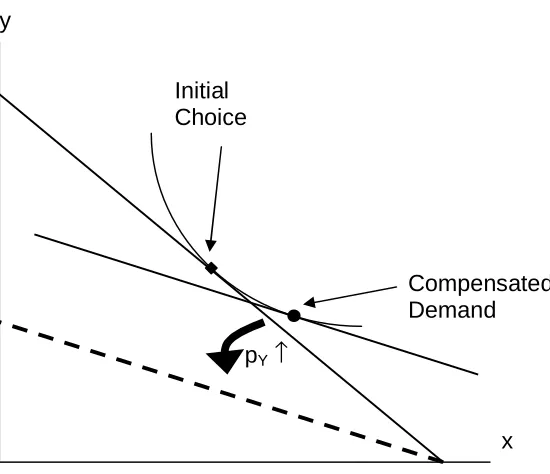
Initial Choice
pY↑
Compensated Choice
qA*
Tax p
q DBefore Tax SBefore Tax
qB*
Tax Revenue
Dead Weight Loss
Dedication to this edition:
For Sophie. Perhaps by the time she goes to university, we’ll have won the war against the publishers.
Author’s Disclaimer:
This is the third draft. Please point out typos, errors or poor exposition, preferably by email to [email protected]. Your assistance matters.
In preparing this manuscript, I have received assistance from many people, including Michael Bernstein, Steve Bisset, Grant Chang-Chien, Lauren Feiler, Alex Fogel, Ben Golub, George Hines, Richard Jones, Jorge Martínez, Joshua Moses, Christopher Robert, Dr. John Ryan, and Wei Eileen Xie. I am especially indebted to Anthony B. Williams for a careful, detailed reading of the manuscript yielding hundreds of improvements.
Dr. Celik’s Disclaimer on the version in use at ESSEC:
McAfee’s textbook is an excellent source for students who know their way around in calculus but who are – relatively speaking – newcomers to economics. Since this is an attempt to “customize” this text for a rather condensed course, the ESSEC version focuses only on the material which can be covered in a period of five – eight weeks, therefore it is much shorter than the 300 plus paged original. In contrast to McAfee’s version, the consumption side of the economy is covered before the production side here. The original text is supplemented with sections which closely follow the coverage in other standard textbooks by Walter Nicholson and Hal R. Varian. An attempt is made to use the terminology and notation that will sound more familiar in ESSEC.
Introduction to Economic Analysis
Customized for ESSEC – Version October 2013
by
R. Preston McAfee
J. Stanley Johnson Professor of
Business, Economics & Management
California Institute of Technology
First Version: June 24, 2004
This book presents introductory economics (“principles”) material using standard mathematical tools, including calculus. It is designed for a relatively sophisticated undergraduate who has not taken a basic university course in economics. It also contains the standard intermediate microeconomics material and some material that ought to be standard but is not. The book can easily serve as an intermediate microeconomics text. The focus of this book is on the conceptual tools and not on fluff. Most microeconomics texts are mostly fluff and the fluff market is exceedingly over-served by $100+ texts. In contrast, this book reflects the approach actually adopted by the majority of economists for understanding economic activity. There are lots of models and equations and no pictures of economists.
This work is licensed under the Creative Commons
Attribution-NonCommercial-ShareAlike License. To view a copy of this license, visit
http://creativecommons.org/licenses/by-nc-sa/2.0/
or send a letter to Creative Commons, 559 Nathan Abbott Way, Stanford, California 94305, USA.
TABLE OF CONTENTS
1 WHAT IS ECONOMICS?... 1-5
1.1.1 Normative and Positive Theories... 1-6 1.1.2 Economic Reasoning and Analysis... 1-7
2 SUPPLY AND DEMAND...2-10
2.1 Supply and Demand...2-10
2.1.1 Demand and Consumer Surplus...2-10 2.1.2 Supply and Profit... 2-15
2.2 The Market...2-20
2.2.1 Market Demand and Supply...2-20 2.2.2 Equilibrium...2-22
2.3 Changes in Supply and Demand... 2-24
2.3.1 Changes in Demand...2-24 2.3.2 Changes in Supply... 2-24
2.4 Elasticities...2-28
2.4.1 Elasticity of Demand...2-28 2.4.2 Elasticity of Supply...2-31 2.4.3 Cross-Price and Income Elasticities... 2-31
3 CONSUMER THEORY ...3-33
3.1 Choice, Preferences, and Utility... 3-33
3.1.1 Axioms of Rational Choice...3-33 3.1.2 Utility Maximization...3-34 3.1.3 Indifference Curves...3-36 3.1.4 Budget or Feasible Set... 3-38 3.1.5 Optimal Choice... 3-41 3.1.6 Examples...3-45 3.1.7 Substitution and Income Effects...3-48 3.1.8 Engel Curve...3-51
3.2 Additional Considerations...3-53
3.2.1 Dynamic Choice... 3-53 3.2.2 Risk...3-58
4 PRODUCER THEORY ...4-62
4.1 The Competitive Firm...4-62
4.1.1 Types of Firms... 4-62 4.1.2 Production Functions...4-64 4.1.3 Opportunity Cost... 4-69 4.1.4 Short Run Cost Minimization...4-70 4.1.5 Long Run Cost Minimization...4-73 4.1.6 Short Run Supply and Equilibrium... 4-77 4.1.7 Long Run Supply and Equilibrium... 4-79 4.1.8 Economies of Scale and Scope...4-80
4.2 Perfect Competition Dynamics... 4-82
4.2.1 Long-run Equilibrium... 4-82 4.2.2 Dynamics with Constant Costs...4-83
5 MARKET IMPERFECTIONS...5-88
5.1 Taxes...5-88
5.1.1 Effects of Taxes...5-88
5.2 Externalities...5-92
5.2.1 Private and Social Value, Cost...5-93 5.2.2 Example: A Production Externality...5-96 5.2.3 Pigouvian Taxes...5-98 5.2.4 Quotas or Permits...5-100 5.2.5 Tradable Permits and Auctions...5-101 5.2.6 Coasian Bargaining...5-102 5.2.7 Example: Tragedy of the Commons...5-105
5.3 Public Goods...5-107
5.3.1 Examples...5-107
5.4 Information...5-108
5.4.1 Market for Lemons...5-109 5.4.2 Signaling...5-110
6 STRATEGIC BEHAVIOR...6-112
6.1 Games...6-112
6.1.1 Matrix Games...6-112 6.1.2 Nash Equilibrium...6-117 6.1.3 Mixed Strategies...6-119 6.1.4 Examples...6-123 6.1.5 Two Period Games...6-126 6.1.6 Subgame Perfection...6-127 6.1.7 Supergames...6-129 6.1.8 The Folk Theorem...6-130
7 INDEX ...7-132
7.1 List of Figures...7-132
1
What is Economics?
Economics studies the allocation of scarce resources among people – examining what goods and services wind up in the hands of which people. Why scarce resources? Absent scarcity, there is no significant allocation issue. All practical, and many impractical, means of allocating scarce resources are studied by economists. Markets are an important means of allocating resources, so economists study markets. Markets include stock markets like the New York Stock Exchange, commodities markets like the Chicago Mercantile, but also farmer’s markets, auction markets like Christie’s or Sotheby’s (made famous in movies by people scratching their noses and inadvertently purchasing a Ming vase) or eBay, or more ephemeral markets, such as the market for music CDs in your neighborhood. In addition, goods and services (which are scarce resources) are allocated by governments, using taxation as a means of acquiring the items. Governments may be controlled by a political process, and the study of allocation by the politics, which is known as political economy, is a significant branch of economics. Goods are allocated by certain means, like theft, deemed illegal by the government, and such allocation methods nevertheless fall within the domain of economic analysis; the market for marijuana remains vibrant despite interdiction by the governments of most nations. Other allocation methods include gifts and charity, lotteries and gambling, and cooperative societies and clubs, all of which are studied by economists.
Some markets involve a physical marketplace. Traders on the New York Stock Exchange get together in a trading pit. Traders on eBay come together in an electronic marketplace. Other markets, which are more familiar to most of us, involve physical stores that may or may not be next door to each other, and customers who search among the stores, purchasing when the customer finds an appropriate item at an acceptable price. When we buy bananas, we don’t typically go to a banana market and purchase from one of a dozen or more banana sellers, but instead go to a grocery store. Nevertheless, in buying bananas, the grocery stores compete in a market for our banana patronage, attempting to attract customers to their stores and inducing them to purchase bananas.
Economic analysis is used in many situations. When British Petroleum sets the price for its Alaskan crude oil, it uses an estimated demand model, both for gasoline consumers and also for the refineries to which BP sells. The demand for oil by refineries is governed by a complex economic model used by the refineries and BP estimates the demand by refineries by estimating the economic model used by refineries. Economic analysis was used by experts in the antitrust suit brought by the U.S. Department of Justice both to understand Microsoft’s incentive to foreclose (eliminate from the market) rival Netscape and consumer behavior in the face of alleged foreclosure. Stock market analysts use economic models to forecast the profits of companies in order to predict the price of their stocks. When the government forecasts the budget deficit or considers a change in environmental regulations, it uses a variety of economic models. This book presents the building blocks of the models in common use by an army of economists thousands of times per day.
1.1.1 Normative and Positive Theories
Economic analysis is used for two main purposes. The first is a scientific understanding of how allocations of goods and services – scarce resources – are actually determined. This is a positive analysis, analogous to the study of electromagnetism or molecular biology, and involves only the attempt to understand the world around us. The development of this positive theory, however, suggests other uses for economics. Economic analysis suggests how distinct changes in laws, rules and other government interventions in markets will affect people, and in some cases, one can draw a conclusion that a rule change is, on balance, socially beneficial. Such analyses combine positive analysis – predicting the effects of changes in rules – with value judgments, and are known as normative analyses. For example, a gasoline tax used to build highways harms gasoline buyers (who pay higher prices), but helps drivers (who face fewer potholes and less congestion). Since drivers and gasoline buyers are generally the same people, a normative analysis may suggest that everyone will benefit. This type of outcome, where everyone is made better off by a change, is relatively uncontroversial.
In contrast, cost-benefit analysis weighs the gains and losses to different individuals and suggests carrying out changes that provide greater benefits than harm. For example, a property tax used to build a local park creates a benefit to those who use the park, but harms those who own property (although, by increasing property values, even non-users obtain some benefits). Since some of the taxpayers won’t use the park, it won’t be the case that everyone benefits on balance. Cost-benefit analysis weighs the costs against the benefits. In the case of the park, the costs are readily monetized (turned into dollars), because the costs to the tax-payers are just the amount of the tax. In contrast, the benefits are much more challenging to estimate. Conceptually, the benefits are the amount the park users would be willing to pay to use the park if the park charged admission. However, if the park doesn’t charge admission, we would have to estimate willingness-to-pay. In principle, the park provides greater benefits than costs if the benefits to the users exceed the losses to the taxpayers. However, the park also involves transfers from one group to another.
not just of the overall gains and losses, but also weighting those gains and losses by their effects on other social goals. For example, a property tax used to subsidize the opera might provide more value than costs, but the bulk of property taxes are paid by lower and middle income people, while the majority of opera-goers are rich. Thus, the opera subsidy represents a transfer from relatively low income people to richer people, which is not consistent with societal goals of equalization. In contrast, elimination of sales taxes on basic food items like milk and bread generally has a relatively greater benefit to the poor, who spend a much larger percentage of their income on food, than to the rich. Thus, such schemes may be considered desirable not so much for their overall effects but for their redistribution effects. Economics is helpful not just in providing methods for determining the overall effects of taxes and programs, but also the incidence of these taxes and programs, that is, who pays, and who benefits. What economics can’t do, however, is say who ought to benefit. That is a matter for society at large to decide.
1.1.2 Economic Reasoning and Analysis
Economic reasoning is rather easy to satirize. One might want to know, for instance, what the effect of a policy change – a government program to educate unemployed workers, an increase in military spending, or an enhanced environmental regulation – will be on people and their ability to purchase the goods and services they desire. Unfortunately, a single change may have multiple effects. As an absurd and tortured example, government production of helium for (allegedly) military purposes reduces the cost of children’s birthday balloons, causing substitution away from party hats and hired clowns. The reduction in demand for clowns reduces clowns’ wages and thus reduces the costs of running a circus. This cost reduction increases the number of circuses, thereby forcing zoos to lower admission fees to compete with circuses. Thus, were the government to stop subsidizing the manufacture of helium, the admission fee of zoos would likely rise, even though zoos use no helium. This example is superficially reasonable, although the effects are miniscule.
To make any sense at all of the effects of a change in economic conditions, it is helpful to divide up the effect into pieces. Thus, we will often look at the effects of a change “other things equal,” that is, assuming nothing else changed. This isolates the effect of the change. In some cases, however, a single change can lead to multiple effects; even so, we will still focus on each effect individually. A gobbledygook way of saying “other things equal” is to use Latin and say “ceteris paribus.” Part of your job as a student is to learn economic jargon, and that is an example. Fortunately, there isn’t too much jargon.
necessarily invalidate the conclusions drawn from the theory, however, for at least four reasons:
• People often make decisions as families or households rather than individuals, and it may be sensible to consider the household as the “consumer.” That households are fairly selfish is more plausible perhaps than individuals being selfish.
• Economics is pretty much silent on why consumers want things. You may want to make a lot of money so that you can build a hospital or endow a library, which would be altruistic things to do. Such motives are broadly consistent with self-interested behavior.
• Corporations are often required to serve their shareholders by maximizing the share value, inducing self-interested behavior on the part of the corporation. Even if corporations had no legal responsibility to act in the financial interest of their shareholders, capital markets may force them to act in the self-interest of the shareholders in order to raise capital. That is, people choosing investments that generate a high return will tend to force corporations to seek a high return. • There are many good, and some not-so-good, consequences of people acting in
their own self-interest, which may be another reason to focus on self-interested behavior.
Thus, while there are limits to the applicability of the theory of self-interested behavior, it is a reasonable methodology for attempting a science of human behavior.
Self-interested behavior will often be described as “maximizing behavior,” where consumers maximize the value they obtain from their purchases, and firms maximize their profits. One objection to the economic methodology is that people rarely carry out the calculations necessary to literally maximize anything. However, that is not a sensible objection to the methodology. People don’t carry out the physics calculations to throw a baseball or thread a needle, either, and yet they accomplish these tasks. Economists often consider that people act “as if” they maximize an objective, even though no calculations are carried out. Some corporations in fact use elaborate computer programs to minimize costs or maximize their profits, and the entire field of operations research is used to create and implement such maximization programs. Thus, while individuals don’t carry out the calculations, some companies do.
The fallacy of sunk costs is often thought to be an advantage of casinos. People who lose a bit of money gambling hope to recover their losses by gambling more, with the sunk “investment” in gambling inducing an attempt to make the investment pay off. The nature of most casino gambling is that the house wins on average, which means the average gambler (and even the most skilled slot machine or craps player) loses on average. Thus, for most, trying to win back losses is to lose more on average.
The way economics is performed is by a proliferation of mathematical models, and this proliferation is reflected in this book. Economists reason with models. Models help by removing extraneous details from a problem or issue, letting one analyze what remains more readily. In some cases the models are relatively simple, like supply and demand. In other cases, the models are relatively complex. In all cases, the models are the simplest model that lets us understand the question or phenomenon at hand. The purpose of the model is to illuminate connections between ideas. A typical implication of a model is “when A increases, B falls.” This “comparative static” prediction lets us see how A affects B, and why, at least in the context of the model. The real world is always much more complex than the models we use to understand the world. That doesn’t make the model useless, indeed, exactly the opposite. By stripping out extraneous detail, the model represents a lens to isolate and understand aspects of the real world.
2
Supply and Demand
Supply and demand are the most fundamental tools of economic analysis. Most applications of economic reasoning involve supply and demand in one form or another. When prices for home heating oil rise in the winter, usually the reason is that the weather is colder than normal and as a result, demand is higher than usual. Similarly, a break in an oil pipeline creates a short-lived gasoline shortage, as occurred in the Midwest region of the United States in the year 2000, which is a reduction in supply. The price of DRAM, or dynamic random access memory, used in personal computers falls when new manufacturing facilities begin production, increasing the supply of memory.
This chapter sets out the basics of supply and demand, introduces equilibrium analysis, and considers some of the factors that influence supply and demand and the effects of those factors. In addition, quantification is introduced in the form of elasticities. The chapters on consumer and producer theories (which will follow this one) will introduce a more fundamental analysis of supply and demand. In essence, the current chapter is the economics “quickstart” guide, and we will look more deeply in the subsequent chapters.
2.1
Supply and Demand
2.1.1 Demand and Consumer Surplus
Eating a French fry makes most people a little bit happier, and we are willing to give up something of value – a small amount of money, a little bit of time – to eat one. What we are willing to give up measures the value – our personal value – of the French fry. That value, expressed in dollars, is the willingness to pay for French fries. That is, if you are willing to give up three cents for a single French fry, your willingness to pay is three cents. If you actually pay a penny for the French fry, you’ve obtained a net of two cents in value. Those two cents – the difference between your willingness to pay and the amount you do pay – is known as consumer surplus. Consumer surplus is the value to a consumer of consumption of a good, minus the price paid.
The value of items – French fries, eyeglasses, violins – is not necessarily close to what one has to pay for them. For people with bad vision, eyeglasses might be worth ten thousand dollars or more, in the sense that if eyeglasses and contacts cost $10,000 at all stores, that is what one would be willing to pay for vision correction. That one doesn’t have to pay nearly that amount means that the consumer surplus associated with eyeglasses is enormous. Similarly, an order of French fries might be worth $3 to a consumer, but because French fries are available for around $1, the consumer obtains a surplus of $2 in the purchase.
or unwilling to eat any more fries even when they are free, which implies that at some point the value of additional French fries is zero.1
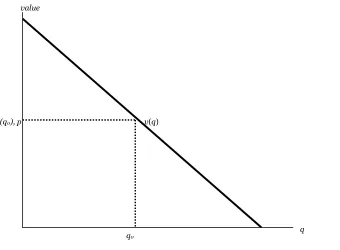
Many, but not all, goods have this feature of diminishing marginal value – the value of the last unit consumed declines as the number consumed rises. If we consume a quantity q, it implies the marginal value v(q) falls as the number of units rise.2 An example is illustrated in Figure 2-1. Here the value is a straight line, declining in the number of units.
Figure 2-1: The Demand Curve
Demand need not be a straight line, and indeed could be any downward-sloping curve. Contrary to the usual convention, demand gives the quantity chosen for any given price off the horizontal axis, that is, given the value p on the vertical axis, the corresponding value q0 on the horizontal axis is the quantity the consumer will purchase.
It is often important to distinguish the demand curve itself – the entire relationship between price and quantity demanded – from the quantity demanded. Typically, “demand” refers to the entire curve, while “quantity demanded” is a point on the curve.
Given a price p, a consumer will buy those units with v(q)>p, since those units are worth more than they cost. Similarly, a consumer should not buy units for which v(q)<p. Thus, the quantity q0 that solves the equation v(q0)=p gives the quantity of units the
1 Sometimes, we will measure consumption as units per period of time, e.g. French fries consumed per
month.
2 When diminishing marginal value fails, which sometimes is said to occur with beer consumption,
constructing demand takes some additional effort, which isn’t of a great deal of consequence. Buyers will still choose to buy a quantity where marginal value is decreasing.
q value
v(q)
q0
consumer will buy. This value is also illustrated in Figure 2-1.3 Another way of summarizing this insight is that the marginal value curve is the inverse of demand function, where the demand function gives the quantity demanded for any given price. Formally, if x(p) is the quantity a consumer buys given a price of p, then v(x(p))=p.
But what is the marginal value curve? Suppose the total value of consumption of the product, in dollar value, is given by u(q). That is, a consumer who pays u(q) for the quantity q is just indifferent to getting nothing and paying nothing. For each quantity, there should exist one and only one price that exactly makes the consumer indifferent between purchasing it and getting nothing at all, because if the consumer is just willing to pay u(q), any greater amount is more than the consumer should be willing to pay.
The consumer facing a price p gets a net value or consumer surplus of CS = u(q) – pq
from consuming q units. In order to obtain the maximal benefit, the consumer would then choose the level of q to maximize u(q) – pq. When the function CS is maximized, its derivative is zero, which implies that, at the quantity that maximizes the consumer’s net value
(
( ))
( ) .0 u q pq u q p
dq d
− ′ = − =
Thus we see that v(q)=u′(q), that is, the marginal value of the good is the derivative of the total value.
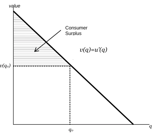
Consumer surplus is the value of the consumption minus the amount paid, and represents the net value of the purchase to the consumer. Formally, it is u(q)-pq. A graphical form of the consumer surplus is generated by the following identity.
(
( ))
( )(
( ))
(
( ))
. max0 0
0 0
0
0 − =
∫
′ − =∫
−= − =
q q
q u q pq u q pq u x pdx v x pdx
CS
This expression shows that consumer surplus can be represented as the area below the demand curve and above the price, as is illustrated in Figure 2-2. The consumer surplus represents the consumer’s gains from trade, the value of consumption to the consumer net of the price paid.
3 We will treat units as continuous, even though in reality they are discrete units. The reason for treating
Figure 2-2: Consumer Surplus
The consumer surplus can also be expressed using the demand curve, by integrating from the price up. In this case, if x(p) is the demand, we have
∫
∞ =p
dy y x
CS ( ) .
When you buy your first car, you experience an increase in demand for gasoline because gasoline is pretty useful for cars and not so much for other things. An imminent hurricane increases the demand for plywood (to protect windows), batteries, candles, and bottled water. An increase in demand is represented by a movement of the entire curve to the northeast (up and to the right), which represents an increase in the marginal value v (movement up) for any given unit, or an increase in the number of units demanded for any given price (movement to the right). Figure 2-3 illustrates a shift in demand.
Similarly, the reverse movement represents a decrease in demand. The beauty of the connection between demand and marginal value is that an increase in demand could in principle have meant either more units demanded at a given price, or a higher willingness to pay for each unit, but those are in fact the same concept – both create a movement up and to the right.
For many goods, an increase in income increases the demand for the good. Porsche automobiles, yachts, and Beverly Hills homes are mostly purchased by people with high incomes. Few billionaires ride the bus. Economists aptly named goods whose demand doesn’t increase with income inferior goods, with the idea that people substitute to better quality, more expensive goods as their incomes rise. When demand for a good
q
value
q0
v(q0)
)()(
quqv
′=
Consumer Surplus
increases with income, the good is called normal. It would have been better to call such goods superior, but it is too late to change such a widely accepted convention.
Figure 2-3: An Increase in Demand
Another factor that influences demand is the price of related goods. The dramatic fall in the price of computers over the past twenty years has significantly increased the demand for printers, monitors and internet access. Such goods are examples of complements. Formally, for a given good X, a complement is a good whose consumption increases the value of X. Thus, the use of computers increases the value of peripheral devices like printers and monitors. The consumption of coffee increases the demand for cream for many people. Spaghetti and tomato sauce, national parks and hiking boots, air travel and hotel rooms, tables and chairs, movies and popcorn, bathing suits and sun tan lotion, candy and dentistry are all examples of complements for most people – consumption of one increases the value of the other. The complementarity relationship is symmetric – if consumption of X increases the value of Y, then consumption of Y
must increase the value of X.4 There are many complementary goods and changes in the prices of complementary goods have predictable effects on the demand of their complements. Such predictable effects represent the heart of economic analysis.
The opposite case of a complement is a substitute. Colas and root beer are substitutes, and a fall in the price of root beer (resulting in an increase in the consumption of root beer) will tend to decrease the demand for colas. Pasta and ramen, computers and typewriters, movies (in theaters) and sporting events, restaurants and dining at home, spring break in Florida versus spring break in Mexico, marijuana and beer, economics
4 The basis for this insight can be seen by denoting the total value in dollars of consuming goods x and y as
u(x, y). Then the demand for x is given by the partial . x u
∂
∂ The statement that y is a complement is the statement that the demand for x rises as y increases, that is, 2 0.
> ∂ ∂ ∂
y x
u But then with a continuous second derivative, 2 0
> ∂ ∂ ∂
x y
u , which means the demand for y,
y u
∂
∂ , increases with x.
q
value
courses and psychology courses, driving and bicycling are all examples of substitutes for most people. An increase in the price of a substitute increases the demand for a good, and conversely, a decrease in the price of a substitute decreases demand for a good. Thus, increased enforcement of the drug laws, which tends to increase the price of marijuana, leads to an increase in the demand for beer.
Much of demand is merely idiosyncratic to the individual – some people like plaids, some like solid colors. People like what they like. Often people are influenced by others – tattoos are increasingly common not because the price has fallen but because of an increased acceptance of body art. Popular clothing styles change, not because of income and prices but for other reasons. While there has been a modest attempt to link clothing style popularity to economic factors,5 by and large there is no coherent theory determining fads and fashions beyond the observation that change is inevitable. As a result, this course, and economics more generally, will accept preferences for what they are without questioning why people like what they like. While it may be interesting to understand the increasing social acceptance of tattoos, it is beyond the scope of this text and indeed beyond most, but not all, economic analyses. We will, however, account for some of the effects of the increasing acceptance of tattoos through changes in the number of firms offering tattooing, changes in the variety of products offered, and so on.
2.1.1.1 (Exercise) A reservation price is the maximum willingness to pay for a good that most people buy one unit of, like cars or computers. Graph the demand curve for a consumer with a reservation price of $30 for a unit of a good.
2.1.1.2 (Exercise) Suppose the demand curve is given by x(p) = 1 – p. The consumer’s expenditure is px(p) = p(1 – p). Graph the expenditure. What price maximizes the consumer’s expenditure?
2.1.1.3 (Exercise) For demand x(p) = 1 – p, compute the consumer surplus function as a function of p.
2.1.1.4 (Exercise) For demand x(p) = pε, for ε <-1, find the consumer surplus as a function of p. (Hint: recall that the consumer surplus can be expressed as
∫
∞ =p
dy y x
CS ( ) .)
2.1.2 Supply and Profit
The supply curve gives the number of units, represented on the horizontal axis, as a function of the price on the vertical axis, which will be supplied for sale to the market. An example is illustrated in Figure 2-4. Generally supply is upward-sloping, because if it is a good deal for a seller to sell 50 units of a product at a price of $10, then it remains a good deal to supply those same 50 at a price of $11. The seller might choose to sell
more than 50, but if the first 50 weren’t worth keeping at a price of $10, that remains true at $11.6
Figure 2-4: The Supply Curve
Exactly in parallel to consumer surplus with demand, profit is given by the difference of the price and the supply curve. This area is shaded in Figure 2-5.
6 This is a good point to remind the reader that the economists’ familiar assumption of “other things
equal” is still in effect. If the increased price is an indication that prices might rise still further, or a consequence of some other change that affects the sellers’ value of items, then of course the higher price might not justify sale of the items. We hold other things equal to focus on the effects of price alone, and then will consider other changes separately. The pure effect of an increased price should be to increase the quantity offered, while the effect of increased expectations may be to decrease the quantity offered.
q p
q0
Figure 2-5: Supplier Profits
The relationship of demand and value exactly parallels the relationship of supply and cost, for a somewhat hidden reason. Supply is just negative demand, that is, a supplier is just the possessor of a good who doesn’t keep it but instead offers it to the market for sale. For example, when the price of housing goes up, one of the ways people demand less is by offering to rent a room in their house, that is, by supplying some of their housing to the market. Similarly, the cost of supplying a good already produced is the loss of not having the good, that is, the value of the good. Thus, with exchange, it is possible to provide the theory of supply and demand entirely as a theory of net demand, where sellers are negative demanders. There is some mathematical economy in this approach, and it fits certain circumstances better than separating supply and demand. For example, when the price of electricity rose very high in the western United States in 2003, several aluminum smelters resold electricity they had purchased in long-term contracts, that is, demanders became suppliers.
However, the “net demand” approach obscures the likely outcomes in instances where the sellers are mostly different people, or companies, than the buyers. Moreover, while there is a theory of complements and substitutes for supply that is exactly parallel to the equivalent theory for demand, the nature of these complements and substitutes tends to be different. For these reasons, and also for the purpose of being consistent with common economic usage, we will distinguish supply and demand.
An increase in supply refers to either more units available at a given price, or a lower price for the supply of the same number of units. Thus, an increase in supply is graphically represented by a curve that is lower or to the right, or both, that is, to the south-east. This is illustrated in Figure 2-6. A decrease in supply is the reverse case, a shift to the northwest.
q p
q0
p
Figure 2-6: An Increase in Supply
Anything that increases costs of production will decrease the supply. For example, as wages rise, the supply of goods and services is reduced, because wages are the input price of labor. Labor accounts for about two-thirds of all input costs, and thus wage increases create supply reductions (a higher price is necessary to provide the same quantity) for most goods and services. Costs of materials of course increase the price of goods using those materials. For example, the most important input into the manufacture of gasoline is crude oil, and an increase of $1 in the price of a 42 gallon barrel of oil increases the price of gasoline about two cents per gallon – almost one-for-one by volume. Another significant input in many industries is capital, and as we will see, interest is cost of capital. Thus, increases in interest rates increase the cost of production, and thus tend to decrease the supply of goods.
Parallel to complements in demand, a complement in supply to a good X is a good Y
such that an increase in the price of Y increases the supply of X. Complements in supply are usually goods that are jointly produced. In producing lumber (sawn boards), a large quantity of wood chips and sawdust are also produced as a by-product. These wood chips and saw dust are useful in the manufacture of paper. An increase in the price of lumber tends to increase the quantity of trees sawn into boards, thereby increasing the supply of wood chips. Thus, lumber and wood chips are complements in supply.
It turns out that copper and gold are often found in the same kinds of rock – the conditions that give rise to gold compounds also give rise to copper compounds. Thus, an increase in the price of gold tends to increase the number of people prospecting for gold, and in the process increases not just the quantity of gold supplied to the market, but also the quantity of copper. Thus, copper and gold are complements in supply.
The classic supply-complement is beef and leather – an increase in the price of beef increases the slaughter of cows, thereby increasing the supply of leather.
The opposite of a complement in supply is a substitute in supply. Military and civilian aircraft are substitutes in supply – an increase in the price of military aircraft will tend to divert resources used in the manufacture of aircraft toward military aircraft and away from civilian aircraft, thus reducing the supply of civilian aircraft. Wheat and corn are also substitutes in supply. An increase in the price of wheat will lead farmers whose land is reasonably well-suited to producing either wheat or corn to substitute wheat for corn, increasing the quantity of wheat and decreasing the quantity of corn. Agricultural goods grown on the same type of land usually are substitutes. Similarly, cars and trucks, tables and desks, sweaters and sweatshirts, horror movies and romantic comedies are examples of substitutes in supply.
Complements and substitutes are important because they are common and have predictable effects on demand and supply. Changes in one market spill over to the other market, through the mechanism of complements or substitutes.
2.1.2.1 (Exercise) A typist charges $30/hr and types 15 pages per hour. Graph the supply of typed pages.
2.1.2.2 (Exercise) An owner of an oil well has two technologies for extracting oil. With one technology, the oil can be pumped out and transported for $5,000 per day, and 1,000 barrels per day are produced. With the other technology, which involves injecting natural gas into the well, the owner spends $10,000 per day and $5 per barrel produced, but 2,000 barrels per day are produced. What is the supply? Graph it.
Hint: Compute the profits, as a function of the price, for each of the technologies. At what price would the producer switch from one technology to the other? At what price would the producer shut down and spend nothing?
2.1.2.3 (Exercise) An entrepreneur has a factory the produces Lα widgets, where α<1, when L hours of labor is used. The cost of labor (wage and benefits) is w per hour. If the entrepreneur maximizes profit, what is the supply curve for widgets?
Hint: The entrepreneur’s profit, as a function of the price, is pLα – wL. The entrepreneur chooses the amount of labor to maximize profit. Find the amount of labor that maximizes, which is a function of p, w and α. The supply is the amount of output produced, which is Lα.
2.1.2.4 (Exercise) In the above exercise, suppose now that more than 40 hours entails a higher cost of labor (overtime pay). Let w be $20/hr for under 40 hours, and $30/hr for each hour over 40 hours, and α = ½. Find the supply curve.
2.1.2.5 (Exercise) In the previous exercise, for what range of prices does employment equal 40 hours? Graph the labor demanded by the entrepreneur.
Hint: The answer involves 10 .
2.1.2.6 (Exercise) Suppose marginal cost, as a function of the quantity q produced, is
mq. Find the producer’s profit as a function of the price p.
2.2
The Market
Individuals with their own supply or demand trade in a market, which is where prices are determined. Markets can be specific or virtual locations – the farmer’s market, the New York Stock Exchange, eBay – or may be an informal or more amorphous market, such as the market for restaurant meals in Billings, Montana or the market for roof repair in Schenectady, New York.
2.2.1 Market Demand and Supply
Individual demand gives the quantity purchased for each price. Analogously, the
market demand gives the quantity purchased by all the market participants – the sum of the individual demands – for each price. This is sometimes called a “horizontal sum” because the summation is over the quantities for each price. An example is illustrated in Figure 2-7. For a given price p, the quantity q1 demanded by one consumer, and the quantity q2 demanded by a second consumer are illustrated. The sum of these quantities represents the market demand, if the market has just those two-participants. Since the consumer with subscript 2 has a positive quantity demanded for high prices, while the consumer with subscript 1 does not, the market demand coincides with consumer 2’s demand when the price is sufficiently high. As the price falls, consumer 1 begins purchasing, and the market quantity demanded is larger than either individual participant’s quantity, and is the sum of the two quantities.
Example: If the demand of buyer 1 is given by q = max {0, 10 – p}, and the demand of buyer 2 is given by q = max {0, 20 – 4p}, what is market demand for the two-participants?
Solution: First, note that buyer 1 buys zero at a price 10 or higher, while buyer 2 buys zero at a price of 5 or higher. For a price above 10, market demand is zero. For a price between 5 and 10, market demand is buyer 1’s demand, or 10 – p. Finally, for a price between zero and 5, the market quantity demanded is 10 – p + 20 – 4p = 30 – 5p.
Figure 2-7: Market Demand
Example: If the supply of firm 1 is given by q = 2p, and the supply of firm 2 is given by q
= max {0, 5p – 10}, what is market supply for the two-participants?
Solution: First, note that firm 1 is in the market at any price, but firm 2 is in the market only if price exceeds 2. Thus, for a price between zero and 2, market supply is firm 1’s supply, or 2p. For p>2, market supply is 5p – 10 + 2p = 7p – 10.
2.2.1.1 (Exercise) Is the consumer surplus for market demand the sum of the consumer surpluses for the individual demands? Why or why not? Illustrate your conclusion with a figure like Figure 2-7.
2.2.1.2 (Exercise) Suppose the supply of firm i is αi p, when the price is p, where i
takes on the values 1, 2, 3, … n. What is the market supply of these n firms?
2.2.1.3 (Exercise) Suppose consumers in a small town choose between two restaurants, A and B. Each consumer has a value vA for A and a value vB for B, each of which is a uniform random draw from the [0,1] interval. Consumers buy whichever product offers the higher consumer surplus. The price of B is 0.2. In the square associated with the possible value types, identify which consumers buy from firm A. Find the demand (which is the area of the set of consumers who buy from A in the picture below). Hint: Consumers have three choices: Buy nothing (value 0), buy from A (value vA – pA) and buy from B, (value vB – pB = vB – 0.2). Draw the lines illustrating which choice has the highest value for the consumer.
p
q1 q2 q1+ q2
2.2.2Equilibrium
Economists use the term equilibrium in the same way as the word is used in physics, to represent a steady state in which opposing forces are balanced, so that the current state of the system tends to persist. In the context of supply and demand, equilibrium refers to a condition where the pressure for higher prices is exactly balanced by a pressure for lower prices, and thus that the current state of exchange between buyers and sellers can be expected to persist.
When the price is such that the quantity supplied of a good or service exceeds the quantity demanded, some sellers are unable to sell because fewer units are purchased than are offered. This condition is called an excess supply, or surplus. The sellers who fail to sell have an incentive to offer their good at a slightly lower price – a penny less – in order to succeed in selling. Such price cuts put downward pressure on prices, and prices tend to fall. The fall in prices generally reduces the quantity supplied and increases the quantity demanded, eliminating the excess supply. That is, an excess supply encourages price cutting, which reduces the excess supply, a process that ends only when the quantity supplied equals the quantity demanded.
Similarly, when the price is low enough that the quantity demanded exceeds the quantity supplied, an excess demand, or shortage exists. In this case, some buyers fail to purchase, and these buyers have an incentive to accept a slightly higher price in order to be able to trade. Sellers are obviously happy to get the higher price as well, which tends to put upward pressure on prices, and prices rise. The increase in price tends to reduce the quantity demanded and increase the quantity supplied, thereby eliminating the e. Again, the process stops when the quantity supplied equals the quantity demanded.
Value of A Value
of B
Price of B
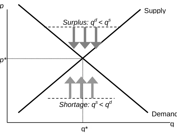
Figure 2-8: Equilibration
This logic, which is illustrated in Figure 2-8, justifies the conclusion that the only equilibrium price is the price in which the quantity supplied equals the quantity demanded. Any other price will tend to rise in an excess demand, or fall in an excess supply, until supply and demand are balanced. In Figure 2-8, an excess supply arises at any price above the equilibrium price p*, because the quantity supplied qs is larger than
the quantity demanded qd. The effect of the excess supply – leading to sellers with
excess inventory – induces price cutting which is illustrated with three arrows pointing down.
Similarly, when the price is below p*, the quantity supplied qs is less than the quantity
demanded qd. This causes some buyers to fail to find goods, leading to higher asking
prices and higher bid prices by buyers. The tendency for the price to rise is illustrated with the arrows pointing up. The only price which doesn’t lead to price changes is p*, the equilibrium price in which the quantity supplied equals the quantity demanded.
The logic of equilibrium in supply and demand is played out daily in markets all over the world, from stock, bond and commodity markets with traders yelling to buy or sell, to Barcelona fish markets where an auctioneer helps the market find a price, to Istanbul gold markets, to Los Angeles real estate markets.
2.2.2.1 (Exercise) If demand is given by qd(p) = a – bp, and supply is given by qs(p) =
cp, solve for the equilibrium price and quantity. Find the consumer surplus and producer profits.
p
q Demand Supply
q*
p*
Surplus: qd < qs
2.2.2.2 (Exercise) If demand is given by qd(p) = apε, and supply is given by qs(p) = bpη,
where ε is negative and η is positive, solve for the equilibrium price and quantity.
2.3
Changes in Supply and Demand
2.3.1 Changes in Demand
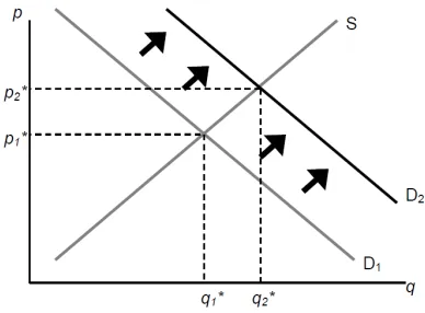
What are the effects of an increase in demand? As the population of California has grown, the demand for housing has risen. This has pushed the price of housing up, and also spurred additional development, increasing the quantity of housing supplied as well. We see such a demand increase illustrated in Figure 2-9, which represents an increase in the demand. In this figure, supply and demand have been abbreviated S and D. Demand starts at D1 and is increased to D2. Supply remains the same. The equilibrium price increases from p1* to p2*, and the quantity rises from q1* to q2*.
Figure 2-9: An Increase in Demand
A decrease in demand – such as occurred for typewriters with the advent of computers, or buggy whips as cars replaced horses as the major method of transportation – has the reverse effect of an increase, and implies a fall in both the price and the quantity traded. Examples of decreases in demand include products replaced by other products – VHS tapes were replaced by DVDs, vinyl records replaced by CDs, cassette tapes replaced by CDs, floppy disks (oddly named because the 1.44 MB “floppy,” a physically hard product, replaced the 720KB, 5 ¼ inch soft floppy disk) replaced by CDs and flash memory drives, and so on. Even personal computers experienced a fall in demand as the market was saturated in the year 2001.
2.3.2Changes in Supply
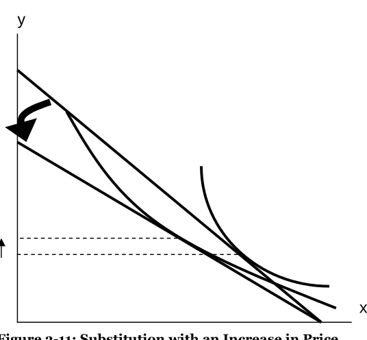
Computer equipment provides dramatic examples of increases in supply. Consider Dynamic Random Access Memory, or DRAM. DRAMs are the chips in computers and many other devices that store information on a temporary basis.7 Their cost has fallen dramatically, which is illustrated in Figure 2-11.8 Note that the prices in this figure reflect a logarithmic scale, so that a fixed percentage decrease is illustrated by a straight line. Prices of DRAMs fell to close to 1/1000th of their 1990 level by 2004. The means by which these prices have fallen are themselves quite interesting. The main reasons are shrinking the size of the chip (a “die shrink”), so that more chips fit on each silicon disk, and increasing the size of the disk itself, so that more chips fit on a disk. The combination of these two, each of which required the solutions to thousands of engineering and chemistry problems, has led to dramatic reductions in costs and consequent increases in supply. The effect has been that prices fell dramatically and quantities traded rose dramatically.
Figure 2-10: An Increase in Supply
An important source of supply and demand changes are changes in the markets of complements. A decrease in the price of a demand-complement increases the demand for a product, and similarly, an increase in the price of a demand-substitute increases demand for a product. This gives two mechanisms to trace through effects from external markets to a particular market via the linkage of demand substitutes or complements. For example, when the price of gasoline falls, the demand for automobiles (a complement) overall should increase. As the price of automobiles rises, the demand for bicycles (a substitute in some circumstances) should rise. When the price of computers falls, the demand for operating systems (a complement) should rise. This gives an operating system seller like Microsoft an incentive to encourage technical progress in the computer market, in order to make the operating system more valuable.
7 Information that will be stored on a longer term basis is generally embedded in flash memory or on a
hard disk. Neither of these products lose their information when power is turned off, unlike DRAM.
Figure 2-11: Price of Storage
An increase in the price of a supply-substitute reduces the supply of a good (by making the alternative good more attractive to suppliers), and similarly, a decrease in the price of a supply complement reduces the supply of a good. By making the by-product less valuable, the returns to investing in a good are reduced. Thus, an increase in the price of DVD-R discs (used for recording DVDs) discourages investment in the manufacture of CD-Rs, which are a substitute in supply, leading to a decrease in the supply of CD-Rs. This tends to increase the price of CD-Rs, other things equal. Similarly, an increase in the price of oil increases exploration for oil, tending to increase the supply of natural gas, which is a complement in supply. However, since natural gas is also a demand substitute for oil (both are used for heating homes), an increase in the price of oil also tends to increase the demand for natural gas. Thus, an increase in the price of oil increases both the demand and the supply of natural gas. Both changes increase the quantity traded, but the increase in demand tends to increase the price, while the increase in supply tends to decrease the price. Without knowing more, it is impossible to determine whether the net effect is an increase or decrease in the price.
2.3.2.1 (Exercise) Video games and music CDs are substitutes in demand. What is the effect of an increase in supply of video games on the price and quantity traded of music CDs? Illustrate your answer with diagrams for both markets.
2.3.2.3 (Exercise) Concerns about terrorism reduced demand for air travel, and induced consumers to travel by car more often. What should happen to the price of Hawaiian hotel rooms?
When the price of gasoline goes up, people curtail their driving to some extent, but don’t immediately scrap their SUVs and rush out and buy more fuel-efficient automobiles or electric cars. Similarly, when the price of electricity rises, people don’t replace their air conditioners and refrigerators with the most modern, energy-saving models right away. There are three significant issues raised by this kind of example. First, such changes may be transitory or permanent, and people reasonably react differently to temporary changes than to permanent changes. The effect of uncertainty is a very important topic and will be considered later, but only in a rudimentary way for this introductory text. Second, energy is a modest portion of the cost of owning and operating an automobile or refrigerator, so it doesn’t make sense to scrap a large capital investment over a small permanent increase in cost. Thus people rationally continue operating “obsolete” devices until their useful life is over, even when they wouldn’t buy an exact copy of that device, an effect with the gobbledygook name of hysteresis. Third, a permanent increase in energy prices leads people to buy more fuel efficient cars, and to replace the old gas guzzlers more quickly. That is, the effects of a change are larger over a larger time interval, which economists tend to call the long-run.
A striking example of such delay arose when oil quadrupled in price in 1973-4, caused by a reduction in sales by the cartel of oil-producing nations, OPEC, which stands for the Organization of Petroleum Exporting Countries. The increased price of oil (and consequent increase in gasoline prices) caused people to drive less and to lower their thermostats in the winter, thus reducing the quantity of oil demanded. Over time, however, they bought more fuel efficient cars and insulated their homes more effectively, significantly reducing the quantity demanded still further. At the same time, the increased prices for oil attracted new investment into oil production in Alaska, the North Sea between Britain and Norway, Mexico and other areas. Both of these effects (long-run substitution away from energy, and long-run supply expansion) caused the price to fall over the longer term, undoing the supply reduction created by OPEC. In 1981, OPEC further reduced output, sending prices still higher, but again, additional investment in production, combined with energy-saving investment, reduced prices until they fell back to 1973 levels (adjusted for inflation) in 1986. Prices continued to fall until 1990, when they were at all-time low levels and Iraq’s invasion of Kuwait and the resulting first Iraqi war sent them higher again.
Short-run and long-run effects represent a theme of economics, with the major conclusion of the theme that substitution doesn’t occur instantaneously, which leads to predictable patterns of prices and quantities over time.
2.4
Elasticities
2.4.1 Elasticity of Demand
Let x(p) represent the quantity purchased when the price is p, so that the function x
represents demand. How responsive is demand to price changes? One might be tempted to use the derivative x′ to measure the responsiveness of demand, since it measures directly how much the quantity demanded changes in response to a small change in price. However, this measure has two problems. First, it is sensitive to a change in units. If I measure the quantity of candy in kilograms rather than pounds, the derivative of demand for candy with respect to price changes even when demand itself has remained the same. Second, if I change price units, converting from one currency to another, again the derivative of demand will change. So the derivative is unsatisfactory as a measure of responsiveness because it depends on units of measure. A common way of establishing a unit-free measure is to use percentages, and that suggests considering the responsiveness of demand in percentage terms to a small percentage change in price. This is the notion of elasticity of demand.9 The elasticity of demand is the percentage decrease in quantity that results from a small percentage increase in price. Formally, the elasticity of demand, which is generally denoted with the Greek letter epsilon ε (chosen to mnemonically suggest elasticity) is
. ) ( ) ( p x p x p dp dx x p p dp x dx ′ = = = ε
Recall that the derivative of the demand function is negative (higher prices – lower quantity demanded). Therefore, when measured by the formula above, elasticity is a negative number.10 First, let’s verify that the elasticity is in fact unit free. A change in
the measurement of x cancels because the proportionality factor appears in both the numerator and denominator. Similarly, if we change the units of measurement of price to replace the price p with r=ap,x(p) is replaced with x(r/a). Thus, the elasticity is
, ) ( ) ( ) / ( 1 ) / ( ) / ( ) / ( p x p x p a r x a a r x r a r x a r x dr d r ′ = ′ = = ε
which is independent of a, and therefore not affected by the change in units. How does a consumer’s expenditure, also known as (individual) total revenue, react to a change in price? The consumer buys x(p) at a price of p, and thus expenditure is TR = px(p). Thus
(
1)
. ) ( ) ( ) ( 1 ) ( ) ( ) ( )( = +ε
′ + = ′ +
= x p
p x p x p p x p x p p x p px dp d
9 The concept of elasticity was invented by Alfred Marshall, 1842-1924, in 1881 while sitting on his roof.
10
Therefore,
. 1 1 = +
ε
TR p
TR dp
d
Table 2-1: Various Demand Elasticities11
Product ε
Salt - 0.1
Matches - 0.1
Toothpicks - 0.1
Airline travel, short-run - 0.1 Residential natural gas, short-run - 0.1 Gasoline, short-run - 0.2 Automobiles, long-run - 0.2
Coffee - 0.25
Legal services, short-run - 0.4 Tobacco products, short-run - 0.45 Residential natural gas, long-run - 0.5 Fish (cod) consumed at home - 0.5 Physician services - 0.6 Taxi, short-run - 0.6 Gasoline, long-run - 0.7
Movies - 0.9
Shellfish, consumed at home - 0.9 Tires, short-run - 0.9 Oysters, consumed at home - 1.1 Private education - 1.1 Housing, owner occupied, long-run - 1.2 Tires, long-run - 1.2 Radio and television receivers - 1.2 Restaurant meals - 2.3 Airline travel, long-run - 2.4 Fresh green peas - 2.8 Foreign travel, long-run - 4.0 Chevrolet automobiles - 4.0 Fresh tomatoes - 4.6
In words, the percentage change of total revenue resulting from a one percent change in price is 1 plus the elasticity of demand. Because it is often possible to estimate the elasticity of demand, the formulae can be readily used in practice. Thus, a one percent
11 From http://www.mackinac.org/archives/1997/s1997-04.pdf; cited sources: Economics: Private and
Public Choice, James D. Gwartney and Richard L. Stroup, eighth edition 1997, seventh edition 1995; Hendrick S. Houthakker and Lester D. Taylor, Consumer Demand in the United States, 1929-1970 (Cambridge: Harvard University Press, 1966,1970); Douglas R. Bohi, Analyzing Demand Behavior
increase in price will increase total revenue when the elasticity of demand is between 0 and -1, which is defined as an inelastic demand. A price increase will decrease total revenue when the elasticity of demand is on the interval (-1, -∞), which is defined as an
elastic demand. The case of elasticity exactly equal to -1 is called unit elasticity, and total revenue is unchanged by a small price change.
Table 2-1 provides estimates on demand elasticities for a variety of products.
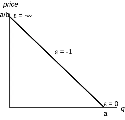
Figure 2-12: Elasticities for Linear Demand
When demand is linear, x(p)=a-bp, the elasticity of demand has the form
.
p b a
p bp
a bp
− − = − − =
ε
This case is illustrated in Figure 2-12.
If demand takes the form x(p)=apε, where ε < 0, then demand has constant elasticity, and the elasticity is equal to ε.
2.4.1.1 (Exercise) Suppose a consumer has a constant elasticity of demand ε, and demand is elastic (ε<-1). Show that expenditure increases as price decreases.
2.4.1.2 (Exercise) Suppose a consumer has a constant elasticity of demand ε, and demand is inelastic (ε>-1). What price makes expenditure the greatest?
2.4.1.3 (Exercise) For a consumer with constant elasticity of demand ε<-1, compute the consumer surplus.
q price
a a/b
ε = -1
ε = 0
2.4.2Elasticity of Supply
The elasticity of supply is analogous to the elasticity of demand, in that it is a unit-free measure of the responsiveness of supply to a price change, and is defined as the percentage increase in quantity supplied resulting from a small percentage increase in price. Formally, if s(p) gives the quantity supplied for each price p, the elasticity of supply, denoted η (the Greek letter “eta”, chosen because epsilon was already taken) is
. ) ( ) ( p s p s p dp ds s p p dp s ds ′ = = = η
Again similar to demand, if supply takes the form s(p)=apη, then supply has constant elasticity, and the elasticity is equal to η. A special case of this form is linear supply, which occurs when the elasticity equals one.
2.4.2.1 (Exercise) For a producer with constant elasticity of supply, compute the producer profits.
2.4.3Cross-Price and Income Elasticities
After defining the elasticity of supply, let us turn back to the demand side one more time. As we saw earlier, price of a good is not the only factor which determines the quantity demanded for that good. Income and prices of related goods affect the purchasing decisions as well. We can extend our discussion of elasticity to quantify these effects.
Suppose that xiis the quantity demanded of good i and pj is the price of the related good
j. Then the cross price elasticity of demand for good i with respect to price of good j is the percentage change in xiwith respect to a 1% increase in pj:
i x j p j dp i dx j p j dp i x i dx
ij = / = /
ε
Notice that this number is positive if goods i and j are substitutes and negative if they are complements.
Similarly, income elasticity of demand is defined as the percentage change in the quantity demanded x corresponding to a 1% increase in income M:
x
M
dM
dx
M
dM
x
dx
M
x
=
/
=
/
,
ε
3
Consumer Theory
Consumer theory is based on what people like. This is something that we can’t directly measure, but must infer. In other words, consumer theory is based on the premise that we can infer what people like from the choices they make.
Now, inferring what people like from choices they make does not rule out mistakes. But our starting point is to consider the implications of a theory in which consumers don’t make mistakes, but make choices that give them the most satisfaction.
Economists think of this approach as analogous to studying gravitation in a vacuum before thinking about the effects of air friction. There is a practical consideration that dictates ignoring mistakes. There are many kinds of mistakes, e.g. “I meant to buy toothpaste but forgot and bought a toothbrush,” a memory problem, “I thought this toothpaste was better but it is actually worse,” a learning issue, and “I meant to buy toothpaste but I bought crack cocaine instead,” a self-control issue. All of these kinds of mistakes lead to distinct theories. Moreover, we understand these alternative theories by understanding the basic theory first, and then seeing what changes these theories lead to.
3.1
Choice, Preferences, and Utility
3.1.1 Axioms of Rational Choice12
One way to begin an analysis of people’s choices is to start with an individual’s “preferences” over different “consumption bundles.” A consumption bundle is a collection of goods and services that the individual might consume. When an individual reports that she “prefers bundle A to bundle B,” she means that all things considered, she feels better off consuming bundle A rather than consuming bundle B. A rational preference relation is assumed to have three basic properties:
I. Completeness: If A and B are any two bundles, the individual can always specify exactly one of the following three possibilities:
1. “A is preferred to B,” 2. “B is preferred to A,” or 3. “A and B are equally go