Love for Quality, Comparative Advantage, and Trade
Esteban Jaimovich Collegio Carlo Alberto
Vincenzo Merella University of Cagliari
This Version: July 2012
First Version: March 2011
Abstract
We propose a Ricardian trade model with horizontal and vertical di¤erentiation, where indi-viduals’willingness to pay for quality rises with their income, and productivity di¤erentials across countries are stronger for high-quality goods. Our theory predicts that the scope for trade widens and international specialisation intensi…es as incomes grow and wealthier consumers raise the quality of their consumption baskets. This implies that comparative ad-vantages intensify gradually over the path of development as a by-product of the process of quality upgrading. The evolution of comparative advantages leads to speci…c trade patterns that change over the growth path, by linking richer importers to more specialised exporters. We provide empirical support for this prediction, showing that the share of imports origi-nating from exporters exhibiting a comparative advantage in a speci…c product correlates positively with the importer’s GDP per head.
Keywords: International Trade, Nonhomothetic Preferences, Quality Ladders.
JEL Classi…cations: F11, F43, O40
We would like to thank Arnaud Costinot, Pablo Fajgelbaum, Giovanni Mastrobuoni, Ignacio Monzon, Alessio
Moro and Ina Simonovska for comments and suggestions, as well as seminar participants at Bologna University,
Collegio Carlo Alberto, University of Surrey, University of Cagliari, Queen Mary, and the Royal Economic Society
1
Introduction
Income is a key determinant of consumer choice. A crucial dimension through which purchasing power in‡uences this choice is the quality of consumption. People with very di¤erent incomes tend to consume commodities within the same category of goods, such as clothes, cars, wines, etc. However, the actual quality of the consumed commodities di¤ers substantially when looking at poorer versus wealthier households. The same reasoning naturally extends to countries with di¤erent levels of income per capita. In this case, the quality dimension of consumption entails important implications on the evolution of trade ‡ows.
Several recent studies have investigated the links between quality of consumption and inter-national trade. One strand of literature has centred their attention on the demand side, …nding a strong positive correlation between quality of imports and the importer’s income per head [Hallak (2006), Fieler (2011a)].1 On the other hand, a set of papers have focused on whether exporters adjust the quality of their production to serve markets with di¤erent income levels. The evidence here also points towards the presence of nonhomothetic preferences along the quality dimension, showing that producers sell higher quality versions of their output to richer importers.2
These empirical …ndings have motivated a number of models that yield trade patterns where richer importers buy high-quality versions of goods, while exporters di¤erentiate the quality of their output by income at destination [Hallak (2010), Fajgelbaum, Grossman and Helpman (2011), Jaimovich and Merella (2012)]. Yet, this literature has approached the determinants of countries’sectoral specialisation as a phenomenon that is independent of the process of quality upgrading resulting from higher consumer incomes. This paper investigates whether exchanging higher or lower quality versions of output a¤ects the categories of goods that countries specialise in, and the intensity of trade links that they establish with di¤erent importers. We propose a theory where quality upgrading in consumption becomes the central driving force behind a general process of comparative advantage intensi…cation and varying bilateral links at di¤erent
1
See also related evidence in Choi, Hummels and Xiang (2009), Francois and Kaplan (1996) and Dalgin,
Trindade and Mitra (2008).
2For example, Verhoogen (2008) and Iacovone and Javorcik (2008) provide evidence of Mexican manufacturing
plants selling higher qualities in US than in their local markets. Brooks (2006) establishes the same results for
Colombian manufacturing plants, and Manova and Zhang (2011) show that Chinese …rms ship higher qualities
of their exports to richer importers. Analogous evidence is provided by Bastos and Silva (2010) for Portuguese
levels of income.
Our theory is grounded on the hypothesis that productivity di¤erentials are stronger for higher-quality goods, combined with the notion that willingness to pay for quality rises with in-come. Within this framework, we show that international specialisation and trade intensify over the growth path. The evolution of trade ‡ows featured by our model presents novel speci…cities that stem from the interaction between nonhomothetic preferences and sectoral productivity di¤erentials that become more pronounced at higher levels of quality. In particular, the process of quality upgrading with rising income sets in motion both demand-driven and supply-driven factors that leads to a simultaneous rise in specialisation by importers and exporters over the growth path. Import and export specialisation take place together precisely because, as coun-tries become richer, consumers shift their spending towards high-quality goods, which are exactly those that tend to display greater scope for export specialisation.
We model a world economy with a continuum of horizontally di¤erentiated goods, each of them available in a continuum of vertically ordered quality levels. Each country produces a particular variety of every good. The production technology di¤ers both across countries and sectors, with some countries being intrinsically better than others in producing certain types of goods. This represents the traditional source of trade in Ricardian models, and leads to specialisation along the horizontal dimension of the commodity space. Alongside this traditional feature, we assume that intrinsic productivity di¤erentials (on the horizontal dimension) tend to become increasingly pronounced as production moves up (vertically) on the quality ladders of each good. In other words, a country may have, for example, a cost advantage in producing wine, while another country may have it in whisky. This would naturally lead them to exchange these two goods. Yet, in our model, productivity di¤erences in the wine and whisky industries do not remain constant along the quality space, but become more intense as production moves up towards higher quality versions of those goods. As a result, the scope for international trade turns out to be wider for high-quality wines and whiskies than for low-quality ones.
leads to a gradual process of increasing international specialisation.
Our model thus suggests that the study of the evolution of trade links may require considering a more ‡exible concept of comparative advantage than the one traditionally used in the literature, so as to encompass quality upgrading as an inherent part of it. In the literature of Ricardian trade, the comparative advantage is solely determined by exporters’ technologies. This paper instead sustains that both the importers’ incomes and the exporters’ sectoral productivities must be taken into account in order to establish a rank of comparative advantage. This is because the degree of comparative advantage between any two countries is crucially a¤ected by the quality of consumption of their consumers. As a consequence, richer and poorer importers may end up establishing trade links with di¤erent partners, simply because the gaps between their willingness-to-pay for quality may translate into unequal degrees of comparative advantage with respect to the same set of exporters.
The conditionality of comparative advantage on importers incomes entails clear and testable predictions on the evolution of trade ‡ows in a growth context. In particular, the model yields predictions that link di¤erent importers to speci…c exporters. According to our model, the share of imports originating from exporters exhibiting an advantage in producing a given good must grow with the income per head of the importer. This would be the result of richer importers buy-ing high-quality versions of goods, which are the type of commodities for which cost di¤erentials across countries are relatively more pronounced. In that regard, we …rst test the notion that productivity di¤erentials become more intense at higher levels of quality of production. Next, we provide evidence consistent with the prediction that richer economies are more likely to buy their imports from producers who display a comparative advantage in the imported goods.
Related Literature
Nonhomothetic preferences are by now a common modelling choice in the trade literature. How-ever, most of the past trade literature with nonhomotheticities has focused either on vertical di¤erentiation [e.g., Flam and Helpman (1987), Stokey (1991) and Murphy and Shleifer (1997)] or horizontal di¤erentiation in consumption [e.g., Markusen (1986), Bergstrand (1990) and Mat-suyama (2000)].3 Two recent articles have combined vertical and horizontal di¤erentiation with
3
For some recent contributions with horizontal di¤erentiation and nonhomothetic preferences see, for example:
Foellmi, Hepenstrick and Zweimuller (2010) and Tarasov (2011), where consumers are subject to a discrete
consumption choice (they must consume either zero or one unit for each good), and Fieler (2011b) who, using a
CES utility function, ties the income elasticity of consumption goods across di¤erent industries to the degree of
preferences featuring income-dependent willingness to pay for quality: Fajgelbaum, Grossman and Helpman (2011) and Jaimovich and Merella (2012).
Fajgelbaum et al. (2011) analyse how di¤erences in income distributions between economies with access to thesame technologies determine trade ‡ows in the presence of increasing returns and trade cost. Like ours, their paper leads to an endogenous emergence of comparative ad-vantages, which may have remained latent for quite some time (either due to trade costs being too high or countries’income distributions being too similar). Our paper, instead, sticks to the Ricardian tradition where trade is the result of di¤ erences in technologies featuring constant returns to scale. In particular, in our model, comparative advantages and trade emerge gradu-ally, not because trade costs obstruct the course of increasing returns, but because the demand for commodities displaying wider heterogeneity in cost of production (i.e., high-quality goods) expands as incomes rise. In that respect, a fundamental di¤erence between the two papers is that in Fajgelbaum et al. (2011) there is no particular reason why high-quality versions of goods are inherently more tradable than low-quality ones (tradeability and specialisation there are essentially determined by di¤erences in the income distributions of countries).
Jaimovich and Merella (2012) also propose a nonhomothetic preference speci…cation where budget reallocations take place both within and across horizontally di¤erentiated goods. That paper, however, remained within a standard Ricardian framework where absolute and com-parative advantages are determined from the outset, and purely by technological conditions. Hence, nonhomothetic preferences play no essential role there in determining export and im-port specialisation at di¤erent levels of development. By contrast, it is the interaction between rising di¤erences in productivity at higher quality levels and nonhomotheticities in quality that generates our novel results in terms of co-evolution of export and import specialisation.
A key assumption in our theory is the widening in productivity di¤erentials at higher levels of quality. To the best of our knowledge, Alcala (2011) is the only other paper that has explicitly introduced a similar feature into a Ricardian model of trade. An important di¤erence between the two papers is that Alcala’s keeps the homothetic demand structure presented in Dornbusch, Fisher and Samuelson (1977) essentially intact. Nonhomotheticities in demand are actually crucial to our story and, in particular, to its main predictions regarding the evolution of trade ‡ows and specialisation at di¤erent levels of income.
and North-South trade. Our model di¤ers from hers in that the e¤ects of demand on trade stem from the allocation of spendingwithin categories of goods rather thanacrossthem.4 Our results therefore hinge on richer consumers switching their good-speci…c expenditure shares from lower-quality to higher-lower-quality versions of the goods. It is in fact thiswithin-good substitution process that leads to our predictions of income-dependent spending shares across di¤erent exporters.5
The rest of the paper is organised as follows. Section 2 studies a world economy with a continuum of countries where all economies have the same level of income per head in equilibrium. Section 3 generalises the main results to a world economy where some countries are richer than others. Section 4 presents some empirical results consistent with the main predictions of our model. Section 5 concludes. All relevant proofs can be found in the Appendices.
2
A world economy with equally rich countries
We study a world economy with a unit continuum of countries indexed by v 2 V. In each country there is a continuum of individuals with unit mass. Each individual is endowed with one unit of labour time. We assume labour is immobile across countries. In addition, we assume all countries are open to international trade, and there are no trading costs of any sort.
2.1 Commodity space and production technologies
All countries share a common commodity space de…ned along three distinct dimensions: a horizontal, avarietal, and avertical dimension.
Concerning the horizontal dimension, there exists a unit continuum of di¤erentiated goods, indexed by z, where z 2 Z = [0;1]. In terms of the varietal dimension, we assume that each countryv2Vproduces a particularvariety vof each di¤erentiated goodz. Finally, our vertical dimension refers to the intrinsic quality of the commodity: a continuum of di¤erent qualities q, where q 2 Q = [1;1), are potentially available for every variety v of each good z. As a result, in our setup, each commodity is designated by a speci…c good-variety-quality index,
(z; v; q)2Z V Q.6 4
This sort of adjustment is absent in her model, as goods there di¤er only on the horizontal dimension.
5In this respect, our paper relates also to Linder (1961) and Hallak (2010) views of quality as an important
dimension in explaining trade ‡ows between countries of similar income levels. We propose a new mechanism
that links together quality of production, income per capita and trade at di¤erent stages of development.
6
In each country v there exists a continuum of …rms that may transform local labour into commodities of variety v. Production technologies are idiosyncratic both to the sector z and to the country v. In particular, we assume that, in order to produce one unit of commodity
(z; v; q), a …rm from country v in sectorz needs to use z;v(q)units of labour, where:
z;v(q) =e z;v
q z;v
1 + , with >0:
Unit labour requirements contain two key technological parameters. The …rst is , which ap-plies identically to all sectors and countries, and we interpret it as the worldwide total factor productivity level.7 The second is z;v, which may di¤er both across z and v, and governs the elasticity of the labour requirements with respect to quality upgrading.8
In what follows, we assume that each parameter z;v is independently drawn from a proba-bility density function with uniform distribution over the interval ; . In addition, we assume that >1. Hence, the labour requirement functions z;v(q) are always strictly increasing and
convex in q.
Henceforth, we denote by wv the wage per unit of labour time in country v. Since in each
sector z of each country v there is a continuum of …rms that are able to produce commodity
(z; v; q)at identical unit cost, in equilibrium, all commodities in the world will be priced exactly at their unit cost. That is,
pz;v;q =e z;v
q z;v
1 + wv; for all (z; v; q)2Z V Q. (1)
2.2 Preferences and budget constraint
All individuals in the world share identical preferences de…ned over the good-variety-quality space described in the previous subsection.
We assume that individuals consume only one quality q 2 Q of each variety v of good z. Henceforth, to ease notation, we denote the consumed quality of variety v of good z simply
The varietal dimension refers to the di¤erent varieties of a given type of good, originating from di¤erent countries,
such as Spanish and French wines (di¤ering in speci…c traits like the types of grapes and regional vini…cation
techniques). The vertical dimension refers to the intrinsic quality of each speci…c commodity (e.g., the ageing and the grapes selection in the winemaking).
7
As such, in our model, increases in will capture the e¤ects of aggregate growth and rising real incomes.
8The multiplicative terme z;v is just included to help simplifying the algebra of the consumer’s optimisation
problem. All our results still hold true when the unit labour requirements are given by z;v(q) =q z;v=(1 + ),
by qz;v. Also, we denote by cz;v 2 R+ the consumed quantity of commodity qz;v. Individual’s
preferences are summarised by the following utility function:
U =
Z
Z
Z
V
lnCz;vdv dz; (2)
with Cz;v=
8 < :
cz;v if cz;v <1; (cz;v)qz;v if cz;v 1:
(3)
Utility U in (2) is de…ned as an additive-separable logarithmic function of the (variety-speci…c) quality-adjusted consumption indicesCz;v de…ned in (3).9 Notice from (3) that Cz;v is
non-decreasing in qz;v, hence quality is always a desirable feature. Moreover, (3) implies that
the quality dimension becomes increasingly desirable as physical consumption rises, since qz;v
only magni…es the utility derived from (physical) consumption when cz;v >1.
An individual with income wwill maximise (2) subject to the following budget constraint:
Z
Z
Z
V
e z;v(qz;v) z;v
1 + wv cz;vdv dz w, (4)
where we have already substituted the price pz;v of each consumed commodity qz;v by its
ex-pression as a function of technological parameters and wage according to (1).
2.3 Utility maximisation
When optimising (2) subject to (4) we must take into account the fact that the consumer’s income may well di¤er across countries. Hereafter, we use the letter i 2 V to refer to the country of origin of a speci…c consumer, and we use i as a superindex any time we refer to
choices made by consumers from countryi.
The consumer’s problem then requires choosing combinations of (non-negative) quantities on the good-variety-quality (three-dimensional) commodity space, subject to (4). However, it turns out that the optimisation problem may be greatly simpli…ed by making use of the following two intermediate results.
9
The additive-separable logarithmic functional form in (2) is posed to ease the exposition. The model delivers
qualitatively identical results under a more general utility function that allows for non-unit degrees of substitution
between the di¤erent commodities(z; v)2Z V. Furthermore, the assumption of a single consumed quality for
each good is also posed to ease exposition, and it corresponds to the solution that arises when assuming anin…nite
degree of substitution between qualities of thesame commodity(z; v)2Z V. More precisely, our results hold qualitatively intact, only at the cost of more tedious algebra, if we replace (2) with the following alternative
function:
U=
(Z
Z Z
V Z
Q
Cz;v(q)dq dv =
dz )1=
First, we may note that the functional form in (3) implies consumers would choose qiz;v >1
only ifciz;v >1 (otherwise the simply setqz;vi = 1).10 As a result, without any loss of generality, we may simply replace the quality-adjusted consumption indicesCz;vi in (2) byCz;vi = ciz;v qz;vi .
Second, by letting iz;v denote henceforth the demand intensity in country i 2 V for the varietyv 2V of goodz 2Z, we may note that ci
z;v = iz;vwi=pz;v (where recall thatpz;v is the
market price of commodityqz;v). Hence, using (1), we may write:
ciz;v =
i z;vwi
e z;v qi
z;v z;vwv=(1 + )
: (5)
The previous two results allow us to restate the original consumer’s optimisation problem into a much simpler one, de…ned only in terms ofoptimal consumed qualities andoptimal budget
allocations across varieties of goods. Below we state thereformulated consumer’s problem.
An individual from country i 2 V chooses the optimal quality qz;vi and optimal budget allocation iz;v for each commodity (z; v)2Z V, so as to solve:11
max
fqi
z;v; iz;vg(z;v)2Z V
U =
Z
Z
"Z
V
qz;vi "
ln (1 + )
i z;v qi z;v z;v wi wv ! + z;v # dv # dz subject to: Z Z Z V i
z;vdv dz= 1; and qz;vi 2Q, for all (z; v)2Z V:
(6)
We can observe that relative wages (wi=wv) may play a role in the optimisation problem (6).
For the time being, we will shut down this channel, and characterise the solution of (6) only for the case in which wages are the same in all countries. (In any case, as it will be shown next, in this speci…cation of the model all wages will turn out to be equal in equilibrium.)
Lemma 1 When wv =w for all v2V, problem (6) yields, for all (z0; v0)2Z V:
qzi0;v0 =
1 +
R
Z
R
Vqz;vi dv dz
!1=( z0;v0 1)
, (7)
i z0;v0 =
(1 + )1=( z0;v0 1)
R
Z
R
Vqz;vi dv dz z0;v0
=( z0;v0 1)
: (8)
In addition,@qzi0;v0=@ >0.
Proof. In Appendix A.
1 0This result follows immediately from (3), which implies thatq
z;vonly magni…es the e¤ect ofcz;vwhencz;v>1
while, according to (1), the pricepz;vis strictly increasing along the quality space.
1 1
Lemma 1 characterises the solution of the consumer’s optimisation problem in terms of two sets of variables: (i) the expressions in (7), which stipulate the quality level in which each variety of every horizontally di¤erentiated good is optimally consumed; (ii) the expressions in (8) describing the optimal expenditure shares allocated to those commodities. Furthermore, the result@qi
z;v=@ >0 summarises the key nonhomothetic behaviour present in our model: quality
upgrading of consumption. That is, the fact that consumers upgrade the quality of all goods they consume as their real incomes grow.
2.4 Equilibrium and specialisation
In equilibrium, total world spending on commodities produced in countryvmust equal the total labour income in country v (which is itself equal to the total value of goods produced in v). Bearing in mind (6), we may then write down the market clearing conditions as follows:
Z
Z
Z
V
i
z;vwidi dz =wv, for all v2V: (9)
More formally, an equilibrium in the world economy is given by a set of wagesfwvgv2Vsuch
that: i) prices of all traded commodities are determined by (1); ii) consumers from country i2 V choose their allocations qz;vi ; iz;v (z;v)
2Z V by solving (6); and iii) the market clearing conditions stipulated in (9) hold simultaneously for all countries.
Proposition 1 Suppose that, for each commodity (z; v) 2 Z V, z;v is independently drawn
from a uniform density function with support ; . Then, for any > 0, in equilibrium:
wv =w for allv 2V.
Proof. In Appendix A.
Proposition 1 shows that, in this (symmetric) world economy, the equilibrium relative wages remain unchanged and equal to unity all along the growth path. The reason for this result is the following: as rises, and real incomes accordingly increase, aggregate demands and supplies grow together at identical speed in all countries. As a consequence, markets clearing conditions in (9) will constantly hold true without the need of any adjustment in relative wages across economies.
country-speci…c processes of labour reallocation across sectors. Such sectoral reallocations of labour stem from the interplay of demand and supply side factors. On the demand side, as real incomes grow with a rising , individuals start consuming higher quality varieties of each commodity –as can be observed from (7). On the supply side, heterogeneities in sectoral labour productivities across countries become stronger as producers intend to raise the quality of their output. Hence, the interplay between income-dependent willingness to pay for quality and the intensi…cation of sectoral productivity di¤erences at higher levels of quality leads to a process of increasing sectoral specialisation as rises.
In what follows we study the e¤ects of the above-mentioned sectoral reallocations of labour on the trade ‡ows across economies. In particular, we focus on the evolution of the revealed comparative advantage (RCA) of every countryv 2Vin each di¤erentiated good z2Z, as we let the worldwide total factor productivity parameter rise.
For every commodity (z; v), we thus compute the ratios:
RCAz;v
Xz;v=Xv
Wz=W
; (10)
whereXz;v (resp. Wz) is the total value of exports of goodz by countryv(resp. by the world),
and Xv (resp. W) is the aggregate value of exports by countryv (resp. by the world).
Since in our model each country sells a negligible share of its own production domestically, we can safely disregard the e¤ect of sales to local consumers and simply write:
Xz;v =
Z
V
i
z;vdi and Xv =
Z
Z
Z
V
i
z;vdi dz:
In addition:
Wz
Z
V
Xz;vdv and W
Z
Z
Wzdz:
Consider …rst the variables relative to country v. We can observe that Proposition 1 implies that iz;v = z;v for all i 2V. Hence, since V has unit measure, Xz;v = z;v. Moreover, from
Proposition 1 and (9), it follows that RZ z;vdz = 1. Therefore, Xv = 1.
Let us look now at the world-level variables, Wz and W. Notice that, by the law of large
numbers, when considering country-speci…c draws, for every goodz2Z, the sequence of sectoral productivity draws z;v v
2V will turn out to be uniformly distributed over the interval ; along the countries space V. As a consequence, the world spending on good z will be equal for all goods, in turn implying that Wz =
R
V z;vdv = 1 for all z 2 Z.12 Furthermore, since
W RZWzdz, we also have thatW = 1.
1 2
Plugging all these results into (10) …nally implies that:
RCAz;v = z;v: (11)
In other words, the revealed comparative advantage of countryvin goodz, which represents our indicator for the degree of export specialisation, is given by the total value of exports of good z by country v. In our symmetric world economy, the total value of exports equals the demand intensity for commodity(z; v), which is identical to all countriesi2Vand may in turn be interpreted as a measure of the degree of import specialisation.
The following proposition characterises in further detail the main properties of each z;v 2
Z Vin this world economy with identical incomes for all countries. Subsequently, we provide some economic interpretation of the formal results in Proposition 2 in terms of both exports and imports specialisation.
Proposition 2 In a symmetric world economy, the value of z;v equals both: (a) the demand
intensity for commodity (z; v) by any country in V; and (b) the RCA of country v in good z.
For any pair of commodities(z0; v0);(z00; v00)2Z V, with z0;v0 < z00v00, the values of z0;v0 and
z00;v00 satisfy the following properties:
(i) z0;v0 > z00;v00.
(ii) @ z0;v0=@ > @ z00;v00=@ .
In addition, de…ning b RZRV z;v z;vdv dz=RZRV z;vdv dz, with z;v qz;v= z;v 1 ,
for z0;v0 <b< z00;v00:
(iii) @ z00;v00=@ <0 and @ z0;v0=@ >0.
Proof. In Appendix A.
The results collected in Proposition 2 characterise the link between sectoral productivities and labour allocations across sectors. Part (i) states that larger shares of resources are allocated to sectors that received better productivity draws (i.e., sectors carrying lower z;v). Next, part (ii) of the proposition establishes that the concentration of resources towards those sectors further intensi…es as world incomes rise. Finally, part (iii) shows that there exists a threshold
b, such that sectors whose z0;v0 <bexperience an increase in their shares when grows, while
the opposite occurs to sectors whose z00;v00>b.
proposition states that countries export more from those sectors where they enjoy higher labour productivity and a stronger RCA. Secondly, by …xing z00 =z0, we may compare a given sector across di¤erent exporters. In this case, recalling (11), we can observe the RCA of exporter v in sectorzturns out to be monotonically linked to the productivity draw z;v: that is, countries that receive better draws for sectorzenjoy a stronger revealed comparative advantage in that sector. In addition, notice that, according to part (ii) of the proposition, both sectoral specialisation and export specialisation intensify as increases over the growth path.
From a demand side perspective, part (ii) of Proposition 2 may be interpreted as a result on increasing import specialisation along the growth path. In particular, from the importer’s perspective (and …xingz00=z0), our model predicts that as economies get richer, for each good z2Z, we observe a process of growing expenditure shares allocated to the varieties ofzproduced by exporters who received better productivity draws in that sector.
The equilibrium characterised in this section has the particular feature that revealed com-parative advantages coincide with demand intensities. This is clearly a very speci…c result that hinges on the assumed symmetry in the distributions of sector-speci…c productivities across countries. The next section shows that this is no longer the case when we introduce some asym-metry across countries. As we will see, although the results discussed here hold qualitatively unchanged, an asymmetric world leads to a richer characterisation of the links between export specialisation, import specialisation and income per capita.
3
A world economy with cross-country inequality
The previous section has dealt with a world economy where, in equilibrium, all countries exhibit the same real income. In this section, we slightly modify the previous setup in order give room for cross-country inequality. On one side, this extension allows us to generalise the previous results concerning export specialisation to a case in which productivity di¤erentials and cost di¤erentials may not always coincide, as a result of equilibrium wages that are di¤erent between some countries. On the other side, introducing cross-country inequality allows us to generate more powerful predictions concerning import specialisation (in terms of export sources) at di¤erent income levels, which we will later on contrast with the data in Section 4.
In what follows we keep the same commodity space and preference structure as those previ-ously used in Section 2. However, we now assume that the world Vis composed by two subsets of countries, each with positive measure. We will refer to the two subsets asregion Handregion
respectively.
Countries in HandLdi¤er in that they face di¤erent random generating processes for their productivity parameters z;v z
2Z. In particular, we assume that, on the one hand, for any
h2 H and everyz2Z, each z;h is independently drawn from a uniform density function with support ; , where >1, just like in the previous section. On the other hand, for any l2 L and everyz2Z, we assume that each z;l= .
Notice that, for countries in region H, this setup keeps intact the fact that we let sectoral productivity di¤erentials become increasingly pronounced at higher levels of quality. However, the current setup also allows for the presence of absolute advantages (at the aggregate level) across subsets of countries, which were absent in the model discussed in Section 2. The next proposition characterises equilibrium wages.
Proposition 3 Suppose that the setVis composed by two disjoint subsets with positive measure:
H andL. Assume that: a) for any(z; h)2Z H, z;h is independently drawn uniform density
function with support ; ; b) for any(z; l)2Z L, z;l= . Then:
(i) for any h2 H, wh=wH;
(ii) for any l2 L, wl=wL;
(iii) wH > wL.
Proof. In Appendix A.
Proposition 3 states that equilibrium wages in region H will be higher than in region L. The intuition for this result is analogous to all Ricardian models of trade with absolute and comparative advantages. Essentially, regionH(which displays an absolute advantage over region
L) will enjoy higher wages than region L, since this is necessary to lower the monetary costs in L, and thus allow countries in L to export enough to countries in Hand keep the trade balance in equilibrium. Henceforth, without loss of generality, we take the wage in region L as
thenumeraire of the economy, and accordingly setwL= 1.
From the results in Proposition 3 it immediately follows that optimal choices will be identical for countries from the same region. That is, for any h0; h00 2 H, we have that hz;v0 = hz;v00 and qh0
z;v = qh
00
z;v, while for any l0; l00 2 L, we have that l
0
z;v = l
00
z;v and ql
0
z;v =ql
00
z;v, in both cases for
(i) Hz;v denotes the demand intensity for (z; v)2Z Vby a consumer from region H; (ii) Lz;v denotes the demand intensity for(z; v)2Z Vby a consumer from regionL.
Recall also that our nonhomothetic preferences imply that the willingness to pay for quality is increasing in the consumer’s income. As a consequence, in the presence of cross-country income inequality, consumers from H purchase higher quality versions than consumers from L. In addition, given the income level, consumers optimally tend to choose a relatively higher quality of consumption for those commodities carrying a relatively lower z;v. The next proposition formally states these results concerning the consumer choice.
Proposition 4 Let qz;vH andqz;vL denote the quality of consumption of commodity (z; v)2Z V
purchased by a consumer from region H and from region L, respectively. Then, in equilibrium:
(i) qH
z;v> qz;vL >1, for all (z; v)2Z V.
(ii) @qz;hH =@ z;h<0 and@qz;hL =@ z;h<0, for all(z; v)2Z H.
In addition, letting i=H; L, and denoting byqiz; (resp. qiz; ) the value of qiz;h corresponding to
the commodity (z; h)2Z H such that z;h = (resp. ):
(iii) qiz;l=qLi for all(z; l)2Z L, withqiz; < qLi < qiz; .
Proof. In Appendix A.
The …rst result in Proposition 4 is a straightforward implication of our nonhomothetic pref-erences: richer consumers choose higher quality versions of all consumed goods.
The second result states that, considering all commodities produced within region H, the quality of consumption within a given country is a monotonically decreasing function of the labour requirement elasticities of quality upgrading z;h. In that regard, notice that since all countries in H have the same wage, when considering only producers from this region, a larger
z;h will map monotonically into a higher market price.
Finally, the third result shows that, for any given level of consumer income, the quality of the goods produced within region L is neither the highest nor the lowest. In particular, the highest quality of each goodz purchased byany consumer is produced in the country of region
Hthat received the best draw, z;h= . Conversely, the lowest quality of each goodzpurchased byany consumer is produced in the country of regionHthat received the worst draw, z;h = . In this last case, despite the fact that all producers fromL received draws equal to , the lower labour cost in L allows them to sell higher qualities than the least e¢ cient producers from H. Nonetheless, in spite of wH > 1, the highest qualities are still provided by the countries with
3.1 Export specialisation
We proceed now to study the patterns of exporters’ specialisation in this world economy with cross-country inequality. Recall the de…nition of the RCA from (10). Notice …rst that the equality of total world demand across all di¤erentiated goods z 2 Z found in Section 2 still holds true when countries di¤er in income. As a consequence, in this version of the model, we have again that Wz =W for all z2Z.
We let 2(0;1) denote the Lebesgue measure of H. We can observe that total exports of goodz by country vare given by
Xz;v = Hz;vwH+ (1 ) Lz;v: (12)
Moreover, integrating over Z, we obtain the aggregate exports by countryv as
Xv = wH
Z
Z
H
z;vdz+ (1 )
Z
Z
L
z;vdz: (13)
Now, notice that since z;l = , we must have that Hz;l = HL and Lz;l = LL, for all
(z; l)2Z L. Hence, denoting byRCAz;lthe revealed comparative advantage of country l2 L
in goodz2Z, using (12) and (13) we obtain:
RCAz;L= 1; for all (z; l)2Z L: (14)
Consider now a country h 2 H. Since all h obtain their draws of z;h from independent U ; distributions, and since all Hz;h are well-de…ned functions of z;h, applying the law of large numbers it follows that the integralsRZ Hz;hdz andRZ Lz;hdz must both yield an identical value for every country h 2 H. Let thus denote HH RZ Hz;hdz and LH RZ Lz;hdz, which using (12) and (13) lead to:
RCAz;h= H
z;hwH+ (1 ) Lz;h
H
HwH+ (1 ) LH
; for any (z; h)2Z H: (15)
Note that the demand intensities iz;h are all strictly decreasing functions of the draws z;h.13
We can then state the following result, which links again the revealed comparative advantage of an exporter of good z to the productivity draw of the exporter in that sector.
Proposition 5 The revealed comparative advantage of country h 2 H in good z 2 Z may
be depicted by a strictly decreasing function of the sectoral productivity draw z;h. Formally,
1 3
RCAz;h = z;h , where z;h : ; ! R+, with 0( ) < 0, ( ) > 1, and ( ) < 1.
Moreover, 9e2 ; such that when z;hQe, then RCAz;h RRCAz;L.
Proof. In Appendix A.
As we did before, by looking at a particular z 2 Z, we may compare the RCA of di¤erent countries in a given sector. We can then observe that Proposition 5 yields an analogous result in terms of export specialisation as Proposition 2: economies with lower z;h draws tend to display stronger RCA in sectorz. Furthermore, producers from the country that received the best pos-sible draw, z;h = , always display the highest observed value ofRCAz;h. However, in contrast
with Proposition 2, in this version of the model the RCA will no longer map monotonically into sectoral absolute advantages. More precisely, since the wage di¤erential between regionsH and Lcreates a wedge between the absolute and the comparative advantage, it is no longer the case thatRCAz;v can be represented by a monotonically decreasing function of the productivity
draw z;v for all v 2 V. In fact, although a country h 2 H with draw e < z;h < displays higher labour productivity in sector z than any country l 2 L, the RCA in sector z of country h is smaller than the one of country l.
Finally notice that, according to Proposition 4, those producers fromHthat received draws
z;h= are also the ones to end up selling the highest qualities of good zin the world markets.
In fact, they sell the highest quality to both consumers fromHandL. As a consequence, merging the results in Proposition 4 and Proposition 5, our model yields an interesting prediction that we will bring to the data in Section 4. Namely, countries that display a stronger revealed comparative advantage in goodz are also those exporting varieties of goodz at higher levels of quality.
3.2 Import Specialisation
We turn now to study the implications of this version of the model in terms of import speciali-sation. For any countryi, the import shares of goodzoriginating from the countryv0 are given by iz;v0=
R
V
i
z;vdv. However, since the consumer’s optimisation problem yields
R
V
i
z;vdv = 1
for all z2Z, we can represent those import shares simply by the demand intensities iz;v0.
Proposition 6 Let Hz; and Lz; denote, respectively, the demand intensity by consumers from
regionHandLfor goods produced by exporters who received a draw z;h= . Then: Hz; > Lz; ,
for all z2Z.
Proposition 6 states that the import share of any particular good originating from exporters exhibiting the highest RCA in that sector are larger in countries from regionHthan in countries from region L. In other words, the share of imports originating from exporters exhibiting the strongest cost advantage in producing a given good should grow with the importer’sper capita income. This is because the nonhomothetic structure of preferences implies that richer importers tend to buy high-quality commodities, while such commodities are those exhibiting wider cost di¤erentials across countries. To the best of our knowledge, this is a novel prediction in the trade literature that has never been tested empirically. In Section 4.2, we provide evidence consistent with the prediction that richer economies are more likely to buy their imports from producers who display a stronger revealed comparative advantage in the imported goods.
3.3 Extension: Cross-country inequality in an N-region world
We consider now an extension to the previous setup where the world is composed by K > 2
regions, indexed by k = 1; :::; K. We let Vk Vdenote the subset of countries from region k,
whereVkhas Lebesgue measure k>0. In addition, we let each country in regionkbe denoted
by a particular vk2 Vk. (The results discussed in this section are formalised in Appendix B.)
Henceforth we assume that for any vk 2 Vk and every z 2 Z, each z;vk is independently
drawn from the following two-step distribution function:
1. with probability( k )=( ), the sectoral productivity is z;vk = k, where k2 ; , and is described in further detail below;
2. with probability ( k)=( ), the value of z;v
k is drawn from a uniform distribution
with support over [ k; ].
We assume that, for any two regions k0< k00, it holds that k0 < k00, while on the extremes:
k=
8 < :
; fork=K; ; fork= 1:
(Notice that if we letK= 2, then this setup would become exactly as the one presented above, withH= 1 and L= 2.)
In this extended setup, equilibrium wages will display an analogous structure as the one described in Proposition 3. Namely, in equilibrium, the wage for all vk 2 Vk will be wk. In
We now use the superindex j = 1;2; :::; K to denote the region of origin of the consumer. (Notice that, since all individuals from the same region earn the same wages, they must choose identical consumption pro…les.) We then let jz;vk denote the demand intensity by a consumer from region Vj for good(z; vk)2Z Vk. It follows then that, for a country vk
Xz;vk =
K
X
j=1
jwj jz;vk:
Moreover, in equilibrium, it must be the case that Xvk = wk for all vk 2 Vk. In addition,
Wz =W for all z2Zis still true in this extended setup. As a result, the RCA of country vk in
goodz is given by
RCAz;vk =
PK
j=1 jwj
j z;vk
wk
: (16)
Since wages di¤er across regions, once again, we cannot …nd a monotonic relationship between RCAz;vk in (16) and the productivity draws z;vk of all countries in the world pooled together.
However, we can still …nd a result analogous to Proposition 5. In particular, it is still true that the highest value ofRCAz;vk corresponds to the country in regionV1 receiving the best possible
draw in sectorz. That is, RCAz;vk is highest for countryv1 with z;v1 = .
Lastly, concerning imports specialisation, this extension also yields a result that is analogous to that in Proposition 6. For the same reasons as discusses in Section 3.2, the demand intensities
j
z;vk equal the import shares in countryjof goodzoriginating from exportervk. Now, following
an analogous notation as in Proposition 6, we can show that 1z; > ::: > kz;0 > ::: > Kz; , where
1 < k0 < K. Again, this result stems from the fact that our preferences are nonhomothetic in quality, hence richer consumers allocate a larger share of their spending in good z to the producers who can most e¢ ciently o¤er higher qualities versions of that good.
4
Empirical analysis
4.1 Exporters behaviour
Our theory is fundamentally based on the assumption that sectoral productivity di¤erentials across countries become wider along their respective quality ladders. In its purest sense, this assumption is really hard to test empirically. However, the intensi…cation of sectoral productivity di¤erentials at higher qualities implies that the degree of specialisation of countries in speci…c goods and the level of quality of their exports should display a positive correlation. In this subsection we aim to provide some evidence consistent with this prediction.
Objective data on products quality is hardly available for a large set of goods.14 For that
reason, we take unit values as a proxy for the quality of the commodity.15 Like in the previ-ous sections, in order to measure the degree of specialisation we use the revealed comparative advantage (RCA). That is, for each exporter x of goodz in year t, we compute the ratio:
RCAz;x;t
(Vz;x;t=Vx;t) (Wz;t=Wt)
;
whereVz;x;t (resp. Wz;t) is the total value of exports of goodzby countryx(resp. by the world)
in yeart, andVx;t (resp. Wt) is the aggregate value of exports by countryx(resp. by the world)
in year t.
We compute unit values of exports using the dataset compiled by Gaulier and Zignano (2010). This database reports monetary values and physical quantities of bilateral trade for years 1995 to 2009 for more than 5000 products categorised according to the 6-digit Harmonised System (HS-6). Monetary values are measured FOB (free on board) in US dollars. We use the same dataset to compute the RCA of each exporter in each particular HS-6 product.
In our model, comparative advantages become stronger at higher levels of quality of produc-tion. Taking unit values as proxy for quality, this implies that theaverage unit values of exports by each country in each of the traded goods should correlate positively with the RCA of the exporter in those goods.
1 4
The only article we are aware of assessing the e¤ects of product quality on export performance using objective
measures of quality is Crozet, Head and Mayer (2011) for the champagne industry in France.
1 5
There is a large literature in trade using unit values as proxy for quality: e.g., Schott (2004), Hallak (2006),
Fieler (2011a). We acknowledge the fact that unit values are not perfect proxies for quality, since other factors
may also a¤ect prices, such as: the degree of horizontal di¤erentiation across industries, heterogeneous transport
costs, trade tari¤s. In addition, as shown by Simonovska (2011), nonhomothetic preferences may induce …rms
to charge variable mark-ups on their products depending on the income level of the importer. See Khandelwal
(2010) and Hallak and Schott (2011) for some innovative methods to infer quality from prices taking into account
To assess this implication, we …rst run the following regression:
log (weighted_mean_Pz;x;t) = + log (RCAz;x;t) + z+ t+ z;x;t: (17)
The dependent variable in (17) is the logarithm of the average unit value of exports across importers, using export shares as weights for each importer’s unit value.16 The regression also includes product dummies z (to control for di¤erent average prices of goods across di¤erent
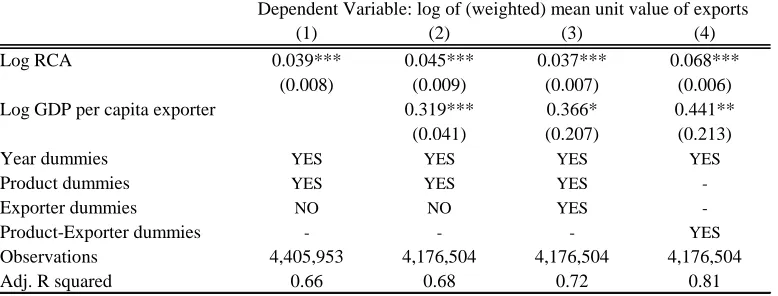
categories of the HS-6 system) and time dummies t(to control for aggregate price levels, which may well di¤er across years). The results of regression (17) are shown in column (1) of Table 1.A. Consistent with our model, the variables log (RCAz;x;t) and log (weighted_mean_Pz;x;t)
display a positive correlation, which is also highly signi…cant.17
It might be the case that the above correlation is simply re‡ecting the fact that more devel-oped economies tend to capture larger markets for their products and, at the same time, tend to produce higher quality versions of the traded products. To account for that possibility, in column (2) we include the logarithm of exporter’s income per capita. As we can observe, the coe¢ cient associated to this variable is indeed positive and highly signi…cant.18 Nevertheless, our estimate of remains essentially unaltered and highly signi…cant, suggesting that the corre-lation between RCA and export unit values is not solely driven by di¤erences in the exporters’ income per head.
In column (3) we add a set of exporter dummies to the regression. The rationale for this is to control for …xed (or slow-changing) exporters’ characteristics (such as, geographic location, institutions, openness to trade) which may somehow a¤ect average export prices, and may be at the same time correlated with export penetration. Our correlation of interest falls a bit in magnitude, but still remains positive and highly signi…cant. Finally, in column (4) we include a
1 6More precisely, the dependent variable is computed as follows:
log (weighted_mean_Pz;x;t) log
X
m2M
vz;x;m;t
vz;x;t
vz;x;m;t
ci;x;m;t
! ;
where: vz;x;m;t (resp. cz;x;m;t) denotes the monetary value (resp. the physical quantity) of exports of goodz,
by exporter x, to importer m, in year t. The summation is across the set of importers, M. To mitigate the
possible contaminating e¤ects of outliers, we have discarded unit values above the 95th percentile and below the
5th percentile for each exporter and product (our results remain essentially intact if we do not trim the price data
at the two extremes of the distribution).
1 7A similar regression is run by Alcala (2011), although for a smaller set of goods (he uses only the apparel
industry) and only using import prices by the US as the dependent variable. The results he obtains are very
similar to ours in Table 1.A.
1 8
(1) (2) (3) (4)
Log RCA 0.039*** 0.045*** 0.037*** 0.068***
(0.008) (0.009) (0.007) (0.006)
Log GDP per capita exporter 0.319*** 0.366* 0.441**
(0.041) (0.207) (0.213)
Year dummies YES YES YES YES
Product dummies YES YES YES
-Exporter dummies NO NO YES
-Product-Exporter dummies - - - YES
Observations 4,405,953 4,176,504 4,176,504 4,176,504
Adj. R squared 0.66 0.68 0.72 0.81
Robust absolute standard errors clustered at the exporter level reported in parentheses. All data is for years 1995-2009. The total number of different products is 5017. * significant at 10%; ** significant at 5%; *** significant at 1%.
TABLE 1.A
Dependent Variable: log of (weighted) mean unit value of exports
full set of product-exporter …xed e¤ects. These dummies would control for …xed characteristics of exporters in speci…c markets: for example, geographic distance from the exporter to the main importers of a given product, the intensity of competition in given industries across di¤erent ex-porters, etc. After including product-exporter dummies, our estimate of the correlation between log of RCA and log of export unit values remains positive and highly signi…cant, rising also in magnitude by a fair amount. In addition, the estimate associated to the exporter’s income per head also remains positive and signi…cant.
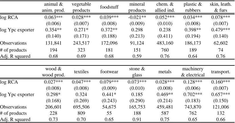
Table 1.A shows pooled regressions for all HS-6 products. However, the correlation of interest may well di¤er across industries. To get a feeling of whether the previous results are mainly driven by particular sectors, we next split the set of HS 6-digit products according to fourteen separate subgroups at the 2-digit level.19 In Table 1.B, we repeat the regression conducted in column (4), but running it separately for each of the 14 subgroups. Although the point estimates for tend to di¤er across subgroups, in all cases they come out positive and highly signi…cant (except for ‘Mineral Products’where it is actually negative and signi…cant). Interestingly (and quite expectably), the point estimates for and for the correlation with the exporter’s income per capita are largest for ‘Machinery/Electrical’and ‘Transportation’products, which comprise manufacturing industries producing highly di¤erentiated products in terms of intrinsic quality.
1 9The subgroups in Table 1.B are formed by merging together subgroups at 2-digit aggregation level, according
to http://www.foreign-trade.com/reference/hscode.htm. We excluded all products within the subgroups
animal & vegetable mineral chem. & plastic & skin, leath. anim. prod. products products allied ind. rubbers & furs log RCA 0.063*** 0.028*** 0.039*** -0.021** 0.052*** 0.034*** 0.078***
(0.006) (0.007) (0.008) (0.009) (0.010) (0.008) (0.007) log Ypc exporter 0.354** 0.271* 0.372** 0.298 0.238 0.398** 0.479***
(0.140) (0.171) (0.188) (0.213) (0.411) (0.194) (0.140) Observations 131,841 243,517 172,096 91,124 483,160 186,173 62,602
# of products 194 323 181 151 760 189 74
Adj. R squared 0.68 0.69 0.68 0.59 0.76 0.64 0.76
wood & stone & machinery
wood prod. glass & electrical
log RCA 0.027*** 0.047*** 0.079*** 0.073*** 0.028*** 0.128*** 0.160*** (0.008) (0.008) (0.009) (0.010) (0.008) (0.006) (0.007) log Ypc exporter 0.298* 0.324 0.441* 0.185 0.469** 0.702*** 0.657***
(0.168) (0.269) (0.243) (0.290) (0.214) (0.183) (0.150) Observations 206,601 695,506 54,675 165,753 459,481 743,870 121,006
# of products 228 809 55 188 587 762 132
Adj. R squared 0.73 0.70 0.65 0.91 0.75 0.65 0.66
Robust absolute standard errors clustered at the exporter level reported in parentheses. All data is for years 1995-2009. All regression include time dummies and product-exporter dummies. * significant 10%; ** significant 5%; *** significant 1%.
textiles footwear metals transport.
foodstuff
TABLE 1.B
4.2 Importers behaviour
Another key aspect of our theory is how imports respond to variations in incomes. The model predicts that changes in incomes will lead to: (i) changes in the quality of consumption, and (ii) changes in the distribution of total production across di¤erent economies. The former result stems from our nonhomothetic preferences, while the latter derives from the interaction between nonhomotheticity and the increasing heterogeneity of sectoral productivities at higher levels of quality.
richer countries should purchase a larger share of their imports of given goods from economies displaying a comparative advantage in those goods.
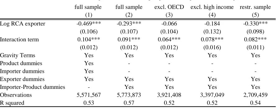
In what follows we aim at providing evidence of such relationship between importer’s income per head and origin of imports. (For computational purposes, given the large number of obser-vations in the panel, in Table 2.A, we use only data from 2009, which is the last year available in the dataset.)20
In Table 2.A, we regress the share of imports of good z by importer m originating from exporter x on the RCA of x in z interacted with the importer’s income per head (Ym). More
precisely, we conduct the following regression (whereimpoz;m;x denotes the value of imports of
good z by importer m originating from exporter x, and X denotes the set of exporters in the sample):
log P impoz;m;x
x2Ximpoz;m;x
= log (RCAz;x) + [log (Ym) log (RCAz;x)]
+Gm;x+ z+ m+"x+ z;x;m:
(18)
Our model predicts a positive value for . This would suggest that richer importers tend to buy a larger share of the imports of goodzfrom exporters exhibiting a comparative advantage in z. Regression (18) includes product dummies ( z), importer dummies ( m), exporter dummies
("x), and a set of bilateral gravity terms (Gm;x) taken from Mayer and Zignano (2006).
Before strictly running regression (18), in column (1) of Table 2.A, we …rst regress the dependent variable of (18) against only the log of the RCA of exporter x in good z (together with product, importer and exporter dummies), which shows as we would expect that those two variables are positively correlated. Secondly, in column (2), we report the results of the regression that includes the interaction term. We can see that the estimated is positive and highly signi…cant, consistent with our theory. Finally, in column (3), we add six traditional gravity terms, and we can observe the previous results remain essentially intact. We can also observe that the estimates for each of the gravity terms are signi…cant, and they all carry the expected sign.
One possible concern with regression (18) is the fact thatRCAz;xis computed with thesame
data that is used to construct the dependent variable. In terms of our estimation of , this could represent an issue if a very large economy turns out to be also a very rich economy (for example, 2 0As robustness checks, we have also run the regressions reported in Table 2.A separately for all the years in
the sample. All the results for years 1995-2008 are qualitatively identical, and very similar in magnitude, to those
the US). In that case, since the imports of goodzby such large and rich economy will be strongly in‡uencing the independent variable RCAz;x, we may be somehow generating by construction
a positive correlation between the dependent variable and [log (Ym) log (RCAz;x)].
In order to deal with this concern, in column (4) we split the set of 184 importers in two separate subsets of 92 importers each (subset A and subset B). When splitting the original set of 184 importers, we do so in such a way the two subsets display similar GDP per capita distributions. (See Appendix C for details and descriptive statistics of the two sub-samples.) We next use the subset A to compute the revealed comparative advantage of each exporter in each product (RCAz;x), while we use the subsetB for the dependent variable in the regression.
By construction, there is therefore no link between the dependent variable in (18) andRCAz;x,
since those two variable are computed with data from di¤erent sets of importers.
As we may readily observe, the results in column (4) of Table 2.A con…rm our previous results in column (3) – the estimate for is positive and highly signi…cant, and of very similar magnitude as in column (3). Lastly, in column (5) we use the RCA computed with the subset A of importers to instrument the RCA used in column (3); again the obtained results con…rm our previous …ndings.21
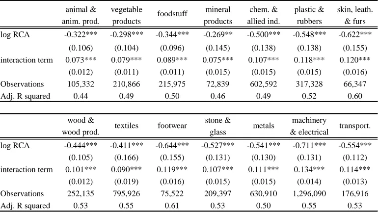
The regressions in Table 2.A pool together more than 5000 6-digit products, implicitly as-suming the same coe¢ cients for all of them. This might actually be a strong assumption to make. In Table 2.B we divide again the 6-digit products into 14 subgroups (the same subgroups we used before in Table 1.B). In the sake of brevity, we report only the estimates for and in (18). As we can observe, the estimates for each subgroup follow a similar pattern as those in Table 2.A; in particular, the estimate associated to the interaction term is always positive and highly signi…cant for each subgroup. As further robustness check, in Table 2.C, we report the percentage of positive and negative estimates for when we run a separate regression for each of the products in the HS 6-digit categorisation.
To conclude, taken jointly, Section 4 yields support to the following ideas: (i) as getting richer, countries tend to raise the quality of the goods they consume (positive correlation between import prices and income per head of importer previously found in the literature); (ii) this, in turn, leads them to raise their import shares originating from exporters displaying a comparative 2 1See Table 2.A (extended) in Appendix C, for some additional robustness checks. There, in column (2) and
(5), we control for product-importer …xed e¤ects (&z;m), instead of z and m separately as in (18). In addition,
in columns (3) and (4) we exclude high income countries from the OECD and high income countries as classi…ed
by the World Bank, to see whether the previous results are mainly driven by the behaviour of richer economies.
Table 2.A
(1) (2) (3) (4) (5) - 2SLS
Log RCA exporter 0.456*** -0.676*** -0.469*** -0.422*** -0.594***
-0.026 (0.138) (0.106) (0.092) (0.129)
Interaction term 0.119*** 0.104*** 0.088*** 0.125***
(0.015) (0.012) (0.010) (0.014)
Distance expo-impo (× 1000) -0.121*** -0.116*** -0.121***
(0.009) (0.010) (0.010)
Contiguity 1.098*** 1.116*** 1.162***
(0.101) (0.131) (0.132)
Common official language 0.362*** 0.413*** 0.436***
(0.099) (0.133) (0.133)
Common coloniser 0.255* 0.164 0.219
(0.152) (0.178) (0.179)
Common legal origin 0.204*** 0.204** 0.222**
(0.082) (0.096) (0.096)
Common currency 0.351** 0.415** 0.408**
(0.149) (0.174) (0.174)
Observations 5,773,873 5,773,873 5,571,567 2,709,459 2,709,459
Number of importers 184 184 184 92 92
R squared 0.47 0.47 0.53 0.51 0.51
Robust absolute standard errors clustered at the importer and exporter level reported in parentheses. All data corresponds to the year 2009.
All regressions include product dummies, importer dummies and exporter dummies. The total number of HS 6-digit products is 5017.
Column (4) uses importers insubset A to compute the exporters' RCA and importers in subset B to compute the dependent variable. Column (5)
uses the RCA computed with importers in subset A to instrument the exporters' RCA. * significant 10%; ** significant 5%; *** significant 1%.
Restricted Sample Dependent Variable: log impo shares of product i from exporterx
Full Sample
Table 2.B
animal & vegetable mineral chem. & plastic & skin, leath. anim. prod. products products allied ind. rubbers & furs log RCA -0.322*** -0.298*** -0.344*** -0.269** -0.500*** -0.548*** -0.622***
(0.106) (0.104) (0.096) (0.145) (0.138) (0.138) (0.155) interaction term 0.073*** 0.079*** 0.089*** 0.075*** 0.107*** 0.118*** 0.120***
(0.012) (0.011) (0.011) (0.015) (0.015) (0.015) (0.016) Observations 105,332 210,866 215,975 72,839 602,592 317,328 66,347 Adj. R squared 0.44 0.49 0.50 0.46 0.49 0.52 0.60
wood & stone & machinery wood prod. glass & electrical
log RCA -0.444*** -0.411*** -0.644*** -0.527*** -0.541*** -0.711*** -0.554*** (0.105) (0.166) (0.155) (0.131) (0.130) (0.131) (0.112) interaction term 0.101*** 0.090*** 0.119*** 0.107*** 0.111*** 0.134*** 0.114***
(0.012) (0.019) (0.016) (0.015) (0.015) (0.014) (0.013) Observations 252,135 795,926 75,522 209,397 630,910 1,296,090 176,916 Adj. R squared 0.53 0.55 0.61 0.53 0.50 0.55 0.53
Robust absolute standard errors clustered at the importer-exporter level in parentheses. All data corresponds to year 2009.
All regression include product, exporter and importer dummies, and the set of gravity terms used before in Table 2.A taken
from Mayer & Zignano (2006). * significant 10%; ** significant 5%; *** significant 1%.
foodstuff
Table 2.C
median
insignificant significant 10% significant 1% insignificant significant 10% significant 1% coefficient
Total number of different products was 4904 (98 products were lost due to insufficient observations). Data corresponds to year 2009 Regressions include importer dummies and the set of gravity terms used in Table 2.A taken from Mayer & Zignano (2006).
Coefficients of Log(Yn) x Log(RCA): independent regressions for each HS 6-digit product
0.076 1.6%
% positive coefficients % negative coefficients
83.5% 16.4%
29.8% 15.7% 38.0% 14.3% 0.5%
advantage in those goods; (iii) this alteration in the origin of imports would re‡ect the fact that these are the exporters relatively more productive at providing higher quality varieties of those goods.
5
Conclusion
We presented a Ricardian model of trade with the distinctive feature that comparative advan-tages reveal themselves gradually over the course of development. The key factors behind this process are the individuals’continuing upgrading in quality of consumption combined with pro-ductivity di¤erentials that widen up as countries seek to increase the quality of their production. As incomes grow and wealthier consumers raise the quality of their consumption baskets, cost di¤erentials between countries become more pronounced. The emergence of such heterogeneities, in turn, alters trade ‡ows, as each economy gradually specialises in producing the subset of goods for which they enjoy a rising comparative advantage.
Our model yielded a number of implications that …nd empirical support. In this respect, using bilateral trade data at the product level, we showed that the share of imports originating from exporters more intensely specialised in a given product correlates positively with GDP per head of the importer. This is consistent with the model’s prediction that richer consumers tend to buy a larger share of their consumption of speci…c goods from countries exhibiting a comparative advantage in those goods. We also provided some evidence supporting the central assumption of our model, namely the intensi…cation of comparative advantage at higher quality levels. In particular, we found that the degree of export specialisation of countries in speci…c goods and the level of quality of their exports display a positive correlation. This fact is consistent with the idea that Ricardian specialisation tends to become more intense at the upper levels of quality of production.
Appendix A: Omitted proofs
Solution of Problem (6). Let i denote the Lagrange multiplier associated to the budget
constraint, and by iz;v the Lagrange multipliers associated to each constraint qz;v 1. Then,
optimisation requires the following FOCs:
ln iz;v z;vlnqiz;v+ ln (1 + ) + ln wi
wv
+ iz;v = 0; for all (z; v)2Z V (19)
qz;vi
i z;v
i = 0; for all (z; v)
2Z V (20)
qiz;v 1 0, iz;v 0, and qz;vi 1 iz;v = 0, for all (z; v)2Z V (21)
Z
Z
Z
V
i
z;vdv dz= 1 (22)
Notice …rst that each (20) may be re-written as qz;vi = i iz;v. Hence, integrating both sides of the equation overZand V, and making use of (22), we may obtain:
Z
Z
Z
V
qz;vi dv dz = i; (23)
which in turn implies that
i
z;v =
qi z;v
i : (24)
Notice also that i 1, sinceqz;vi 1 and bothZand V have unit mass.
Lemma 2 If wv =w for all v2V, then iz;v = 0 for all(z; v)2Z V and all i2V.
Proof. Replacing (24) into (19), and noting thatwi =wwhenwv =wfor allv2V, we obtain:
ln (1 + ) + iz;v = z;v 1 lnqz;vi + ln i; for all (z; v)2Z V: (25)
Now, suppose that there exist(z0; v0) and(z00; v00)such that i
z0;v0 > iz00;v00 = 0. Then, from (21)
and (25) it follows that iz0;v0 = ln i ln (1 + )> z00;v00 1 lnqzi00;v00+ ln i ln (1 + ), but
this is impossible since z00;v00>1and qzi00;v00 1.
Alternatively, suppose that iz;v >0 for all(z; v)2Z V. Then, because of (21) we have that qz;vi = 1 for all(z; v)2Z V, which in turn leads to i= 1 owing to (23). However, this means thatln (1 + ) + iz;v= 0, which is impossible when iz;v >0 because >0. As a result, it must be the case that when wv =w for all v 2 V, then iz;v = 0 holds for all (z; v) 2Z V and all