Changes in between-group inequality:
computers, occupations, and international trade
∗
Ariel Burstein
UCLA
Eduardo Morales
Princeton University
Jonathan Vogel
Columbia University
September 13, 2016
Abstract
We quantify the impact of several determinants of changes in US between-group in-equality. We use an assignment framework with many labor groups, equipment types, and occupations in which changes in inequality are driven by changes in workforce composition, occupation demand, computerization, and labor productivity. We pa-rameterize the model using direct measures of computer usage within labor group-occupation pairs and quantify the impact of each shock for between-group inequality between 1984 and 2003. We find that the combination of computerization and shifts in occupation demand account for roughly 80% of the rise in the skill premium, with computerization alone accounting for roughly 60%. In an open economy extension of the model, we show how computerization and changes in occupation demand may be caused by changes in the extent of international trade and quantify its impact on US inequality. Moving to autarky in equipment goods and occupation services in 2003 reduces the skill premium by 2.2 and 6.5 percentage points, respectively.
1
Introduction
The last few decades have witnessed pronounced changes in relative average wages across groups of workers with different observable characteristics (between-group inequal-ity). Most notably, the wages of workers with more education relative to those with less and of women relative to men have increased substantially in the United States.
A large literature has emerged studying how changes in relative supply and demand for labor groups shape their relative wages. Changes in relative demand across labor groups have been linked prominently to computerization (or a reduction in the price of equipment more generally)—see e.g. Krusell et al. (2000), Autor and Dorn (2013), and
Beaudry and Lewis (2014)—and to changes in relative demand across occupations and
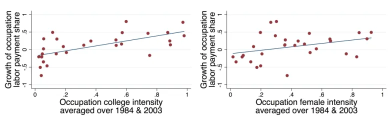
sectors, driven by structural transformation, offshoring, and international trade—see e.g. Autor et al. (2003), Buera et al. (2015), and Galle et al. (2015). Consistent with the first hypothesis, Table 1 shows that computer use rose dramatically between 1984 and 2003 and that computers are used more intensively by educated workers and women. Con-sistent with the second hypothesis, Figure1shows that education- and female-intensive occupations grew relatively quickly over the same time period.1
1984 1989 1993 1997 2003
All 27.4 40.1 49.8 53.3 57.8
Gender Female 32.8 47.6 57.3 61.3 65.1 Male 23.6 34.5 43.9 47.0 52.1 Education College degree 45.5 62.5 73.4 79.8 85.7 No college degree 22.1 32.7 41.0 43.7 45.3
Table 1: Share of hours worked with computers
We contribute to this literature by providing a unifying framework to simultaneously quantify these different determinants of between-group inequality. We use the model to-gether with detailed data on factor allocations to assess the impact of computerization and changes in occupation demand on between-group inequality in the United States. We additionally quantify the extent to which computerization and changes in occupation demand are driven by international trade in equipment goods and occupation output. We base our analysis on an assignment model with many groups of workers and many occupations—building onLagakos and Waugh (2013) andHsieh et al.(2016)—which we extend to incorporate many types of equipment (such as computers) and international trade in occupation services and equipment goods. This framework allows for potentially
Figure 1: Growth (1984-2003) of the occupation share of labor payments and the average (1984 & 2003) of the share of workers in the occupation who have a college degree (left) and are female (right)
rich patterns of complementarity between computers, labor groups and occupations and, in spite of its high dimensionality, remains tractable enough to perform aggregate coun-terfactuals in a parsimonious manner. The model’s aggregate implications for relative wages nest those of workhorse models of between-group inequality in a closed economy, e.g. Katz and Murphy (1992) and Krusell et al. (2000), and in an open economy, e.g. Heckscher-Ohlin.
In our model, the impact of changes in the economic environment on between-group inequality in a given country is shaped by comparative advantage between labor groups, equipment types, and occupations in that country, and comparative advantage across countries in different equipment types and occupations. Consider, for example, the po-tential impact of computerization, modeled as a reduction in the relative price of com-puters (driven by e.g. an increase in productivity of comcom-puters or a reduction in trade costs) on the relative wage of a labor group—such as educated workers or women—that uses computers intensively. A labor group may use computers intensively for two rea-sons. First, it may have a comparative advantage with computers, in which case this group would use computers relatively more within occupations, as is the case for more educated workers in the US. Our model predicts that a reduction in the price of comput-ers increases the relative wage of this labor group. Second, a labor group may have a comparative advantage in occupations in which computers have a comparative advan-tage, in which case this group would be allocated disproportionately to occupations in which all workers are relatively more likely to use computers, as is the case for women in the US. Our model predicts that a reduction in the price of computers may increase or decrease the relative wage of this group depending on the degree of substitutability between occupations.
econ-omy version of the model in which equipment prices and occupation demand shifters are taken as primitives, we conduct a decomposition of changes in relative wages between labor groups in the US between 1984 and 2003. Second, in an open economy extension of the model, we quantify the impact of international trade in equipment goods and oc-cupation services on US relative wages in this time period, as well as the counterfactual impact that moving to autarky would have on US relative wages.
For both of these exercises we must identify comparative advantage between US labor groups, equipment types, and occupations, estimate the elasticity of substitution between occupations, and estimate an elasticity shaping the within-worker dispersion of produc-tivity across occupation-equipment type pairs. Comparative advantage can be inferred directly from data on the allocation of workers to equipment type-occupation pairs. In or-der to estimate the two key elasticities, we or-derive moment conditions that are consistent with equilibrium relationships generated by our model.
To conduct the decomposition exercise, we also must measure computerization as well as changes in occupation demand, labor supply, and labor productivity in the US for the period 1984 to 2003. Changes in equipment productivity that result in comput-erization can be inferred from changes in the allocation of workers to computers within labor group-occupation pairs; focusing on changes within labor group-occupation pairs is important because aggregate computer usage will rise even in the absence of changes in equipment productivity if either labor groups that have a comparative advantage us-ing computers or occupations that have a comparative advantage with computers grow. Occupation demand shifters can be inferred from changes in the allocation of workers to occupations within labor group-equipment type pairs and in labor income shares across occupations. Changes in labor composition are directly observed in the data. Finally, we measure labor productivity as a residual to match changes in the average wage of each labor group.
each worker’s time at work spent using computers; and it only covers the period 1984-2003.2
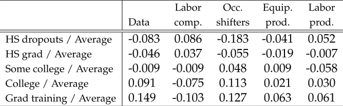
In our decomposition exercise, our model predicts that computerization alone ac-counts for roughly 60% of all shocks that have had a positive impact on the skill pre-mium (i.e. the relative wage of workers with a college degree to those without) between 1984 and 2003 and plays a similar role in explaining disaggregated measures of between-education-group inequality (e.g., the wage of workers with graduate training relative to the average wage). Our model’s prediction is driven by the following three facts observed in the data. First, there has been a large rise in the share of workers using computers within labor group-occupation pairs, which our model interprets as a large increase in computer productivity (i.e. computerization). Second, more educated workers use com-puters within occupations relatively more than less educated workers, which our model interprets as educated workers having a comparative advantage with computers. This pattern of comparative advantage, together with computerization, yields a rise in the rel-ative wages of educated workers according to our model. Third, more educated workers are also disproportionately employed in occupations in which all workers use computers relatively intensively. This pattern of sorting across occupations, together with computer-ization and an estimated elasticity of substitution between occupations greater than one, also yields a rise in the relative wages of educated workers according to our model.
The combination of computerization and occupation shifters accounts for roughly 80% of the rise in the skill premium, leaving only 20% to be explained by labor productivity. This is remarkable, given that we measure changes in labor productivity as a residual that allows our framework to exactly match observed changes in relative wages. We find that computerization, occupation shifters, and labor productivity all play important roles in accounting for the reduction in the gender gap (i.e. the relative wage of male to female workers). Computerization decreases the gender gap because women are disproportion-ately employed in occupations in which all workers use computers intensively and our estimate of the elasticity of substitution across occupations is larger than one.
Whereas in our closed economy model we treat computerization and changes in oc-cupation demand as primitives, in sections 5 and 6 we study the extent to which these changes are a consequence of international trade. Theoretically, we show that the pro-cedure to quantify the impact on relative wages of moving to autarky in equipment and
2The period 1984-2003, however, accounts for a substantial share of the increase in the skill premium
occupation trade is equivalent to the procedure we follow in our closed economy model to calculate the impact of domestic shocks on relative wages, with the only difference that the computerization and occupation demand shocks are now measured as functions of import shares of absorption and export shares of output of different equipment types and occupations. For example, if occupation ω has a high import share relative to
oc-cupation ω0, then moving to autarky has an equivalent impact on relative wages in a
closed economy as increasing domestic occupation demand for ω relative to ω0. Given
the lack of data on the occupation content of exports and imports, measuring occupa-tion trade shares is a challenge; for a full discussion of the difficulties, seeGrossman and Rossi-Hansberg(2007). Given these challenges, we consider alternative simple, albeit im-perfect, approaches to measure the occupation content of exports and imports. Using our preferred approach, we find that moving from 2003 trade shares to equipment (occupa-tion) autarky would generate a 2.2 (6.5) percentage point reduction in the skill premium. We also provide a simple procedure to quantify the differential effects on wages in a given country of changes in primitives (i.e. worldwide technologies, labor compositions, and trade costs) between two time periods relative to the effects of the same changes in primitives if that country were a closed economy. Using this latter result, we quantify the impact of trade in equipment goods and occupation services on between-group inequality in the US between 1984 and 2003. We find that equipment (occupation) trade accounts for roughly 13 percent (27 percent) of the rise in the skill premium between 1984 and 2003 accounted for by changes in equipment productivity (occupation demand) in our closed economy calculations.
Our paper is organized as follows. In Section 2, we discuss the related literature. We describe our closed economy framework, characterize its equilibrium, and discuss its mechanisms in Section 3. We parameterize the model and present our closed economy results in Section4. We extend our model to incorporate international trade in equipment goods and occupation services in Section5and quantify the impact of international trade in Section 6. We conclude in Section 7. Additional details and robustness exercises are relegated to appendices.
2
Literature
assignment of workers to occupations and equipment types. This crucially allows us to study within a unified framework the impact of occupation demand shifters, computer productivity, labor productivity, labor composition, and trade costs on relative average wages of multiple groups of workers, such as the decline in the gender gap and the rise in the skill premium.3
In trying to explain the evolution of between-group inequality as a function of changes in observables, our paper’s objective is most similar to Krusell et al.(2000) andLee and Wolpin(2010). Krusell et al. (2000) estimate an aggregate production function that per-mits capital-skill complementarity and show that changes in aggregate stocks of equip-ment, skilled labor, and unskilled labor can account for much of the variation in the US skill premium. Whereas Krusell et al.(2000) identify the degree of capital-skill comple-mentarity using aggregate time series data, our approach leverages information on the allocation of workers to computers and occupations and, consequently, yields parameter estimates shaping the degree of equipment-labor group complementarity that are robust to allowing for time trends in the relative productivity of each labor group; seeAcemoglu (2002) for a discussion of the relevance of allowing for these time trends in this context. Our decomposition corroborates the findings inKrusell et al.(2000) and extends them by additionally considering the impact of equipment productivity growth on the gender gap and other measures of between-group inequality.
Lee and Wolpin (2010) use a dynamic model of endogenous human capital
accumu-lation and find that labor group productivity (also treated as a residual in their analysis) plays the central role in explaining changes in the skill premium. By considering a greater degree of disaggregation in occupations and labor groups, our results reduce the role of changes in the residual in shaping changes in the skill premium. On the other hand, in contrast toLee and Wolpin(2010), we treat labor composition as exogenous.4
3The relative importance of between- and within-group inequality is an area of active research.Autor
(2014) concludes: “In the US, for example, about two-thirds of the overall rise of earnings dispersion be-tween 1980 and 2005 is proximately accounted for by the increased premium associated with schooling in general and postsecondary education in particular.” On the other hand,Helpman et al.(Forthcoming) con-clude: “Residual wage inequality is at least as important as worker observables in explaining the overall level and growth of wage inequality in Brazil from 1986-1995.”
4Extending our model to endogenize education and labor participation—maintaining a static
environ-ment—would give rise to the same equilibrium equations determining factor allocations and wages condi-tional on labor composition. Our measures of shocks—to occupation shifters, equipment productivity, and labor productivity—and our estimates of model parameters are therefore robust to extending our model to endogenize the supply of each labor group in a static environment. Through the lens of this model, our counterfactual results would be interpreted as the direct effect of shocks to occupation shifters, equipment productivity, and labor productivity on labor demand and wages, taking labor composition as given.. If we also wanted to take into consideration the accumulation of occupation-specific human capital as in, e.g.,
In modeling international trade, we operationalize in a quantitative setting the the-oretical insights of Costinot and Vogel (2010), Sampson (2014), and Costinot and Vogel (2015) regarding the impact of international trade on inequality in high-dimensional en-vironments. We show that one can use a similar approach to that introduced by Dekle et al.(2008) in a single-factor trade model—i.e. replacing a large number of unknown pa-rameters with observable allocations in an initial equilibrium—in a many-factor assign-ment model. In this respect, our paper is compleassign-mentary to concurrent work quantifying the impact of international trade on between-group inequality; see e.g. Adao(2015), Dix-Carneiro and Kovak(2015),Galle et al.(2015), andLee(2016). Relative to this concurrent work, we introduce equipment in the framework and quantify the impact of trade both in equipment and in occupations on inequality; however, relative to this work we only use data for one region: the US. Whereas a large literature has emerged to argue that trade in occupation (or even task) output is a potentially important force generating changes in inequality—see e.g. Grossman and Rossi-Hansberg (2008)—there has been much less work conducting model-based counterfactuals to quantify the importance of this phe-nomenon.5 Given the crudeness of our measures of occupation trade, our quantification of the impact of trade in occupations should be viewed as a first step rather than the final word. Our modeling of international trade in equipment extends the quantitative anal-yses of Burstein et al. (2013) and Parro (2013), who study the impact of trade in capital equipment on the skill premium using the model ofKrusell et al.(2000).
Two related papers use differences in regional exposure to computerization to study the differential effect across regions of technical change on the polarization of US em-ployment and wages,Autor and Dorn(2013), and on the gender gap and skill premium,
Beaudry and Lewis (2014). Our approach complements these papers, embedding
com-puterization into a general equilibrium model that allows us to quantify by means of counterfactual exercises the effect of computerization (as well as other shocks) on changes in between-group inequality.6
the October CPS does not contain this information) and model the corresponding dynamic optimization problem that workers would solve when deciding which occupation to sort into.
5Traiberman(2016) quantifies the impact of import competition on occupation demand and wages. He
constructs a measure of import exposure by occupation by allocating observed sectoral imports to occu-pations according to the share of labor payments going to each occupation in each industry. As we argue below, this measure is likely to be biased if, within industries, certain occupations are more traded than others. Instead of studying inequality,Goos et al.(2014) measure the impact of offshoring on the growth of occupations using data from sixteen European countries imposing a common effect of occupation offshora-bility on changes in occupation size independently of whether a country is a net exporter or a net importer in this occupation. Our model (analogous to the Heckscher-Ohlin model) emphasizes the importance of accounting for differences across countries in comparative advantage and, hence, distinguishing whether a country is a net exporter or importer of each occupation
The approach that we use to bring our model to the data does not require mapping occupations into observable characteristics such as those introduced inAutor et al.(2003). Instead, we estimate measures of comparative advantage and occupation-specific de-mand shocks that vary flexibly across occupations, independently of the similarity in the task composition of these occupations. Even though the information on the task composi-tion of occupacomposi-tions is never used in our analysis, we show in AppendixH.1that changes in the size of occupations are not driven only by occupation demand shifters. For ex-ample, computerization generates an expansion in those occupations that happen to be intensive in non-routine cognitive analytical and interpersonal tasks and a contraction in occupations that are intensive in non-routine manual physical tasks.
In exploiting data on workers’ computer usage, our paper is related to an earlier liter-ature studying the impact of computer use on wages; see e.g. Krueger(1993) andEntorf et al. (1999). This literature identifies the impact of computer usage on wages by re-gressing wages of different workers on a dummy for computer usage, an identification approach thatDiNardo and Pischke(1997) criticize. Our approach to estimate key model parameters does not rely on such a regression. We rely instead on an estimating equation first suggested by Acemoglu and Autor (2011) as an example of how their assignment model might be brought to the data.
3
Closed economy model
In this section we introduce the closed economy version of our model, characterize its equilibrium, and provide intuition for how different changes in the economic environ-ment affect relative wages.
3.1
Environment
At timetthere is a continuum of workers indexed byz ∈ Zt, each of whom inelastically supplies one unit of labor. We divide workers into a finite number of labor groups, in-dexed byλ. The set of workers in groupλis given byZt(λ) ⊆ Zt, which has massLt(λ).
There is a finite number of equipment types, indexed byκ. Workers and equipment are
employed by production units to produce a finite number of occupations, indexed byω.
A final good is produced combining the services of occupations according to a con-stant elasticity of substitution (CES) production function
Yt =
∑
ωµt(ω)1/ρYt(ω)(ρ−1)/ρ
!ρ/(ρ−1)
, (1)
whereρ >0 is the elasticity of substitution across occupations,Yt(ω) ≥0 is the
endoge-nous output of occupation ω, andµt(ω) ≥ 0 is an exogenous demand shifter for
occu-pation ω.7 The final good is used to produce consumption, Ct, and equipment, Yt(κ),
according to the resource constraint
Yt =Ct+
∑
κ˜
pt(κ)Yt(κ), (2)
where ˜pt(κ)denotes the cost of a unit of equipmentκin terms of units of the final good.8
Occupation services are produced by perfectly competitive production units. A unit hiring k units of equipment type κ and l efficiency units of labor group λ produces
kα[T
t(λ,κ,ω)l]1−α units of output, where α denotes the output elasticity of equipment
in each occupation andTt(λ,κ,ω)denotes the productivity of an efficiency unit of group λ’s labor in occupation ω when using equipment κ.9 Comparative advantage between
labor and equipment is defined as follows: λ0 has a comparative advantage (relative
to λ) using equipment κ0 (relative to κ) in occupation ω if Tt(λ0,κ0,ω)/Tt(λ0,κ,ω) ≥
Tt(λ,κ0,ω)/Tt(λ,κ,ω). Labor-occupation and equipment-occupation comparative
ad-vantage are defined symmetrically.
A workerz∈ Zt(λ)suppliese(z)×ε(z,κ,ω)efficiency units of labor if teamed with
equipment κ in occupation ω. Each worker is associated with a unique e(z), allowing
7We show in Sections5 and6that changes in the extent of international trade in occupation services
generate endogenous changes in occupation demand shifters,µt(ω).
8We show in sections5and6how changes in the extent of international trade in equipment generate
endogenous changes in equipment prices ˜pt(κ). Our assumption that equipment must be produced every
period (five-years in our quantitative analysis) is equivalent to assuming that equipment fully depreciates every period. Alternatively, we could have assumed thatYt(κ)denotes investment in capital equipmentκ,
which depreciates at a given finite rate. All our counterfactual exercises are consistent with this alternative model with capital accumulation: they would correspond to comparisons across balanced growth paths in which the real interest rate and the growth rate of relative productivity across equipment types are constant over time.
9We can extend the model to incorporate other inputs such as structure or intermediate inputss;
how-ever, they would not affect any of our results as long as they are produced linearly using the final good and enter the production function multiplicatively ass1−ηkα[T
t(λ,κ,ω)l]1−α
η
. Notice that, in either case,α
is the share of equipment relative to the combination of equipment and labor. We restrictαto be common
some workers withinZt(λ) to be more productive than others across all possible(κ,ω);
we normalize the average value ofe(z)across workers within eachλto be one and prove
this is without loss of generality in Appendix A. Each worker is also associated with a vector of ε(z,κ,ω), one for each (κ,ω) pair, allowing workers within Zt(λ) to vary in
their relative productivities across (κ,ω) pairs. We impose two restrictions. First, the
distribution ofe(z)has finite support and is independent of the distribution ofε(z,κ,ω)
for each (κ,ω). Second, eachε(z,κ,ω)is drawn independently from a Fréchet
distribu-tion with cumulative distribudistribu-tion funcdistribu-tion G(ε) = exp ε−θ, where a higher value of θ > 1 implies lower within-worker dispersion of efficiency units across (κ,ω) pairs.10
The assumption thatε(z,κ,ω) is distributed Fréchet is made for analytical tractability; it
implies that the average wage of a labor group is a CES function of occupation prices and equipment productivity.11
Total output of occupation ω, Yt(ω), is the sum of output across all units producing
occupation ω. All markets are perfectly competitive and all factors are freely mobile
across occupations and equipment types.
Relation to alternative frameworks. Whereas our framework imposes strong restrictions
on occupation production functions, its aggregate implications for wages nest those in Katz and Murphy(1992) andKrusell et al.(2000). Specifically, the aggregate implications of our model for relative wages are equivalent to those inKatz and Murphy(1992) if we assume no equipment (i.e. α = 0) and two labor groups, each of which has a positive
productivity in only one occupation. Similarly, the aggregate implications of our model for relative wages are equivalent to those inKrusell et al.(2000) if we allow for only two labor groups and one type of equipment, each labor group has positive productivity in only one occupation and the equipment share is positive in only one occupation.
3.2
Equilibrium
We characterize the competitive equilibrium, first taking occupation prices as given and then in general equilibrium. Additional derivations are provided in AppendixA.
Partial equilibrium. With perfect competition, equation (2) implies that the price of
equipment κ is simply pt(κ) = p˜t(κ)Pt, where Pt is the price of the final good, which 10SeeAdao(2015) for an approach that relaxes these two restrictions in an environment in which each
worker faces exactly two choices. In AppendixGwe show that our results are robust to allowing for specific forms of statistical dependence of ε(z,κ,ω)across(κ,ω)pairs. Moreover, we also conduct our analysis
allowing for variation across labor groups in the dispersion parameterθand show that our quantitative
results are robust.
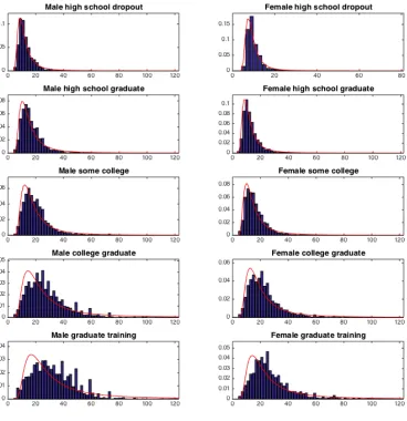
11The wage distribution implied by this assumption is a good approximation to the observed
we normalize to one so that pt(κ) = p˜t(κ). An occupation production unit hiringkunits
of equipmentκandl efficiency units of laborλearns revenues pt(ω)kα[Tt(λ,κ,ω)l]1−α
and incurs costs pt(κ)k+vt(λ,κ,ω)l, wherevt(λ,κ,ω)is the wage per efficiency unit of
laborλ when teamed with equipmentκ in occupationω and pt(ω) is the price of
occu-pationωoutput. The profit maximizing choice of equipment quantity and the zero profit
condition—due to costless entry of production units—yield
vt(λ,κ,ω) = α¯pt(κ)
−α
1−α pt(ω) 1
1−α Tt(λ,κ,ω)
if there is positive entry in (λ,κ,ω), where ¯α ≡ (1−α)αα/(1−α). Facing the wage
pro-file vt(λ,κ,ω), each worker z ∈ Zt(λ) chooses the equipment-occupation pair (κ,ω)
that maximizes her wage,e(z)ε(z,κ,ω)vt(λ,κ,ω). The assumption thatε(z,κ,ω)is
dis-tributed Fréchet and independent of e(z) implies that the probability that a randomly
sampled worker,z∈ Zt(λ), uses equipmentκin occupationωis
πt(λ,κ,ω) =
h
Tt(λ,κ,ω)pt(κ)
−α
1−α pt(ω) 1 1−α
iθ
∑κ0,ω0 h
Tt(λ,κ0,ω0)pt(κ0)
−α
1−α pt(ω0) 1 1−α
iθ. (3)
The higher isθ—i.e. the less dispersed are efficiency units across(κ,ω)pairs—the more
responsive are factor allocations to changes in prices or productivities. According to equa-tion (3), comparative advantage shapes factor allocations. As an example, the assignment of workers across equipment types within any given occupation satisfies
Tt(λ0,κ0,ω)
Tt(λ0,κ,ω)
Tt(λ,κ0,ω)
Tt(λ,κ,ω) =
πt(λ0,κ0,ω) πt(λ0,κ,ω)
πt(λ,κ0,ω) πt(λ,κ,ω)
1/θ ,
so that, ifλ0workers (relative toλ) have a comparative advantage usingκ0(relative toκ)
in occupationω, then they are relatively more likely to be allocated toκ0in occupationω.
The wage per efficiency unit of laborλwhen teamed with equipmentκin occupation ω,vt(λ,κ,ω), differs from theaverage wageof workers in groupλteamed with equipment κin occupationω, denoted bywt(λ,κ,ω), which is the integral ofe(z)ε(z,κ,ω)vt(λ,κ,ω)
across workers teamed with κ in occupation ω, divided by the mass of these workers.
Given our assumptions one(z)and ε(z,κ,ω), we obtain
wt(λ,κ,ω) = αγ¯ Tt(λ,κ,ω)pt(κ)
−α
1−α pt(ω) 1
1−α πt(λ,κ,ω)−1/θ,
or occupation price,Tt(λ,κ,ω) or pt(ω), or a decrease in equipment price, pt(κ), raises
the wages of infra-marginal λ workers allocated to (κ,ω). However, the average wage
across all λ workers in (κ,ω) increases less than that of infra-marginal workers due to
self-selection, i.e. πt(λ,κ,ω)increases, which lowers the average efficiency units of theλ
workers who choose to use equipmentκin occupationω.
Denoting by wt(λ) the average wage of workers in group λ(i.e. total income of the
workers in group λ divided by their mass), the previous expression and equation (3)
implywt(λ) =wt(λ,κ,ω)for all(κ,ω), where12
wt(λ) = αγ¯
∑
κ,ω
Tt(λ,κ,ω)pt(κ)
−α
1−α pt(ω) 1 1−α
θ!1/θ
. (4)
General equilibrium. In any period, occupation prices pt(ω) must be such that total
expenditure in occupationω is equal to total revenue earned by all factors employed in
occupationω,
µt(ω)pt(ω)1−ρEt = 1
1−αζt(ω), (5)
where Et ≡ (1−α)−1∑λwt(λ)Lt(λ)is total expenditure (which equals total income in a closed economy) andζt(ω) ≡ ∑λ,κwt(λ)Lt(λ)πt(λ,κ,ω)is total labor income in
oc-cupation ω. The left-hand side of equation (5) is expenditure on occupation ω and the
right-hand side is total income earned by factors employed in occupation ω. In
equilib-rium, the aggregate quantity of the final good is such thatYt =Et, the aggregate quantity of equipmentκis
Yt(κ) = 1
pt(κ) α
1−α λ
∑
,ωπt(λ,κ,ω)wt(λ)Lt(λ),and aggregate consumption is determined by equation (2).
3.3
System in changes
To solve for changes in wages in response to changes in the economic environment, we express the system of equilibrium equations described in Section3.2in changes, denoting
12The implication that average wagelevelsare common across occupations withinλ(which is
inconsis-tent with the data) obviously implies that the changes in wages will also be common across occupations withinλ. In AppendixIwe decompose the observedchangesin average wages for eachλinto a between
changes in any variablexbetween any two periodst0 andt1 by ˆx ≡ xt1/xt0. Changes in
average wages are given by
ˆ
w(λ) =
∑
κ,ω
ˆ
T(λ,κ,ω)pˆ(κ)
−α 1−αpˆ(ω)
1 1−α
θ
πto(λ,κ,ω)
!1/θ
(6)
and changes in occupation prices are determined by the following system of equations
ˆ
π(λ,κ,ω) =
h ˆ
T(λ,κ,ω)pˆ(κ)
−α 1−αpˆ(ω)
1 1−α
iθ
∑κ0,ω0 h
ˆ
T(λ,κ0,ω0)pˆ(κ0)
−α
1−αpˆ(ω0) 1 1−α
iθ
πt0(λ,κ0,ω0)
(7)
ˆ
µ(ω)pˆ(ω)1−ρEˆ = 1
ζt0(ω)
∑
λ,κwt0(λ)Lt0(λ)πt0(λ,κ,ω)wˆ(λ)Lˆ (λ)πˆ (λ,κ,ω), (8)
and where Eˆ = ∑λ wt0(λ)Lt0(λ)
(1−α)Et0 wˆ(λ)Lˆ (λ). In this system, the forcing variables are: L(ˆ λ),
ˆ
T(λ,κ,ω), µˆ(ω), and pˆ(κ). Given these variables, equations (6)-(8) yield the model’s implied values of changes in average wages, w(λ)ˆ , allocations, πˆ (λ,κ,ω), occupation
prices,pˆ(ω), and total expenditure,Eˆ.
3.4
Intuition
The impact of shocks on wages. According to equation equation (6), changes in
produc-tivities ˆT(λ,κ,ω) and in the price of equipment ˆp(κ) have a direct effect (i.e. holding
occupation prices constant) on wages. In addition, both these shocks as well as changes in occupation shifters and in labor composition affect wages indirectly through their im-pact on equilibrium occupation prices ˆp(ω). The importance of changes in productivities,
equipment prices, and occupation prices for changes in groupλ’s average wage depends
on factor allocations in the initial period,πt0(λ,κ,ω). For example, an increase in
occu-pation ω’s price or a reduction in the price of equipment κ between t0 and t1 raises the
relative average wage of labor groups that disproportionately work in occupation ω or
use equipmentκin periodt0.
We now discuss in more detail the intuition for the impact of each of the shocks (the forcing variables) we consider in our quantitative analysis below. Consider an increase in the occupation demand, i.e. ˆµ(ω) > 1. This shock raises the price of occupation ω
and, therefore, the relative wage of labor groups that are disproportionately employed in occupationω. Similarly, a decrease in labor supply, i.e. ˆL(λ)<1, raises the relative price
wage not only of groupλ, but also of other labor groups employed in similar occupations
as λ.13 A proportional increase across all (κ,ω) in labor productivity for group λ—i.e.
ˆ
T(λ,κ,ω) = Tˆ (λ) > 1—directly raises the relative wage of group λ and reduces the
relative price of occupations in which this group is disproportionately employed, thus reducing the relative wage of labor groups employed in similar occupations asλ.14
Consider the impact of a decrease in the price of equipment κ, i.e. ˆp(κ) < 1, or a
proportional increase in its productivity across all (λ,ω), i.e. ˆT(λ,κ,ω) = Tˆ(κ) > 1.
The impact of these two shocks being equivalent, we focus on a reduction in the price of equipmentκ for illustration purposes. The partial equilibrium impact of this shock is to
raise the relative wage of labor groups that useκ intensively. In general equilibrium this
shock also reduces the relative price of occupations in which κ is used intensively,
low-ering the relative wage of labor groups that are disproportionately employed in these oc-cupations. Overall, the impact on relative wages of changes in equipment price depends on the value ofρand on whether aggregate patterns of labor allocation across equipment
types are mostly a consequence of variation in labor-equipment comparative advantage or mainly determined by variation in labor-occupation and equipment-occupation com-parative advantage. Let us consider two extreme cases.
If the only form of comparative advantage is between workers and equipment, then a decrease in the price ofκ does not affect relative occupation prices (since all occupations
are equally intensive in κ) and, therefore, the effect conditional on maintaining fixed
oc-cupation prices is the same as the general equilibrium effect: a decrease in the price ofκ
will increase the relative wages of worker groups that use equipmentκmore intensively
in the initial period.
If there is no comparative advantage between workers and equipment but there is comparative advantage between workers and occupations and between equipment and occupations, then a decrease in the price of κ has two opposite effects on the relative
wages of worker groups that use equipment κ intensively; i.e. those disproportionately
employed inκ-intensive occupations. While it has a positive effect conditional on
occu-pation prices, it has a negative effect indirectly through its effect on occuoccu-pation prices. The relative strength of the direct and indirect channels depends on ρ. The direct effect
dominates if and only if ρ > 1. Intuitively, a decrease in the price of κ acts like a
pos-13In AppendixD.5we provide empirical evidence that supports our model’s implication that changes
in labor composition affect wages only indirectly through occupation prices.
14Costinot and Vogel(2010) provide analytic results on the implications for relative wages of changes
in labor composition,Lt(λ), and occupation demand,µt(ω), in a restricted version of our model in which
there are no differences in efficiency units across workers in the same labor group (i.e. θ = ∞), there is
no capital equipment (i.e. α = 0), and T(λ,ω)—i.e. ourT(λ,κ,ω)in the absence of equipment—is
itive productivity shock to the occupations in which κ has a comparative advantage. If ρ > 1, this increases employment and the relative wages of labor groups
disproportion-ately employed in the occupations in whichκhas a comparative advantage. The opposite
is true ifρ < 1. In our framework computerization can hence either contract or expand
employment in occupations that are computer intensive.
More generally—outside of these two extreme cases—a decrease in the price of com-puters can simultaneously raise the wage (relative to the average wage) of one labor group (λ1) that uses computers intensively while reducing the wage (relative to the
aver-age waver-age) of another labor group (λ2) that uses computers intensively. This would be the
case ifλ1has a comparative advantage using computers,λ2has a comparative advantage
in the occupations in which computers have a comparative advantage, andρ <1.
The role of θ and ρ. The parameter θ, which governs the degree of within-worker
dis-persion of productivity across occupation-equipment type pairs, determines the extent of worker reallocation in response to changes in occupation prices, equipment prices, and productivities: a higher dispersion of idiosyncratic draws, as given by a lower value ofθ,
results in less worker reallocation. In order to gain intuition on the role ofθfor changes in
labor group average wages, we take a first-order approximation of equation (6) at period
t0allocations:
log ˆw(λ) =
∑
κ,ω
πt0(λ,κ,ω)
log ˆT(λ,κ,ω) + 1
1−αlog ˆp(ω)− α
1−αlog ˆp(κ)
. (9)
This expression shows that, given changes in occupation and equipment prices as well as productivities, the change in average wages does not depend on θ up to a first-order
approximation.15 However, a lower value ofθ results in less worker reallocation across
occupations in response to a shock and, therefore, larger changes in occupation prices. Hence, to a first-order approximation, the value ofθaffects the response of average wages
to shocks by affecting occupation price changes.
The parameterρdetermines the elasticity of substitution between occupations, with a
higher value of ρreducing the responsiveness of occupation prices to shocks and hence,
reducing the impact through occupation price changes of shocks on relative wages. For example, because labor composition only affects relative wages through occupation prices, a higher value ofρreduces the impact of changes in labor composition on relative wages.
Similarly, as described above, a higher value ofρreduces the negative effects of
comput-15More generally, given changes in occupation prices, the shape of the distribution ofε(z,κ,ω)—which
we have assumed to be Fréchet—does not matter for the first-order effect of any shock on average wage changes. The reason is that, for any worker groupλ, the marginal worker’s wage is equal across
erization on wages of labor groups with a comparative advantage on occupations that use computers intensively.
4
Decomposition
In this section we use our closed economy model to quantify the impact of computer-ization, changes in labor composition, changes in occupation demand, and changes in a labor-group specific productivity on observed changes in relative wages in the US. Throughout this section we assume thatTt(λ,κ,ω)can be expressed as
Tt(λ,κ,ω) ≡Tt(λ)Tt(κ)Tt(ω)T(λ,κ,ω). (10)
Accordingly, whereas we allow labor group, Tt(λ), equipment type, Tt(κ), and
occu-pation, Tt(ω), productivity to vary over time, we impose that the interaction between
labor group, equipment type, and occupation productivity, T(λ,κ,ω), is constant over
time. We therefore assume that comparative advantage is fixed over time. This restric-tion allows us to separate cleanly the impact on relative wages ofλ-, κ-, and ω-specific
productivity shocks.16
Given restriction (10), the system in changes given in equations (6)-(8) simplifies to
ˆ
w(λ)=T(ˆ λ) "
∑
κ,ω(qˆ(ω)qˆ(κ))θπt0(λ,κ,ω)
#1/θ
(11)
ˆ
π(λ,κ,ω)= (qˆ(ω)qˆ(κ))
θ
∑κ0,ω0(qˆ(ω0)qˆ(κ0)) θ
πt0(λ,κ0,ω0)
(12)
ˆ
a(ω)qˆ(ω)(1−α)(1−ρ)Eˆ = ∑λ,κwt0(λ)Lt0(λ)πt0(λ,κ,ω)wˆ (λ) ˆ
L(λ)πˆ(λ,κ,ω)
ζt0(ω)
. (13)
In this simplified system, equipment productivity, Tt(κ), is combined with equipment
prices,pt(κ), to form a composite equipment productivity measure: qt(κ) ≡ pt(κ)
−α
1−α Tt(κ).
Similarly, occupation productivity, Tt(ω), is combined with occupation demand,µt(ω),
to form a composite occupation shifter: at(ω) ≡ µt(ω)Tt(ω)(1−α)(ρ−1). Finally,
occupa-tion productivity,Tt(ω), is combined with occupation prices, pt(ω), to form transformed
occupation prices: qt(ω) ≡ pt(ω)1/(1−α)Tt(ω). In this system, the forcing variables
(shocks) are: (i) L(ˆ λ), which we refer to as labor composition; (ii) qˆ(κ), which we refer
16Our results are robust when we perform a set of decompositions that relax this restriction in Appendix
to as equipment productivity; (iii) aˆ(ω), which we refer to as occupation shifters; and (iv) ˆ
T(λ), which we refer to aslabor productivity. Given these shocks, equations (11)-(13) yield the model’s implied values of changes in average wages, w(λ)ˆ , allocations, πˆ (λ,κ,ω),
transformed occupation prices,qˆ(ω), and total expenditure,Eˆ.17
According to equations (11)-(13), we need the following ingredients to perform our decomposition. First, we require measures of factor allocations, πt0(λ,κ,ω), average
wages, wt0(λ), labor composition, Lt0(λ), and labor payments by occupation, ζt0(ω).
We describe the data we employ to obtain each of these measures in Section 4.1. Sec-ond, we require measures of relative shocks to labor composition, ˆL(λ)/ ˆL(λ1),
occupa-tion shifters, ˆa(ω)/ ˆa(ω1), equipment productivity to the powerθ, ˆq(κ)θ/ ˆq(κ1)θ, and labor
productivity, ˆT(λ)/ ˆT(λ1).18 We describe our approach to measure these shocks in
Sec-tion4.2. Finally, we require estimates ofα, ρ, andθ. We describe our estimation strategy
to assign values to these parameters in Section4.3. Finally, we combine these ingredients and describe the results of our decomposition exercise in Section4.4.
4.1
Data
We use data from the Combined CPS May, Outgoing Rotation Group (MORG CPS) and the October CPS Supplement (October Supplement) for the years 1984, 1989, 1993, 1997, and 2003. We restrict our sample by dropping workers who are younger than 17 years old, do not report positive paid hours worked, or are self employed. After cleaning, the MORG CPS and October Supplement contain data for roughly 115,000 and 50,000 individuals, respectively, in each year.19
We divide workers into thirty labor groups by gender, education (high school dropouts, high school graduates, some college completed, college completed, and graduate train-ing), and age (17-30, 31-43, and 44 and older). We consider two types of equipment: computers and other equipment. We use thirty occupations, which we list, together with summary statistics, in Table9in AppendixB.
17The two components of equipment productivity,T
t(κ)and pt(κ), could be measured separately
us-ing information on equipment prices, which are subject to known quality-adjustment issues raised by, e.g.,
Gordon(1990). Similarly, the two components of the occupation shifter,Tt(ω)andµt(ω), could be
mea-sured separately using information on occupation prices, which are hard to measure in practice. If the aim of our exercise were not to determine the impact of observed changes in the economic environment on observed wages but rather to predict the impact of counterfactual or hypothetical changes in the economic environment, then it would not be necessary to combine changes in equipment productivity and equip-ment production costs into a single shock or to combine changes in occupation demand and occupation productivity into a single composite shock.
18In AppendixC we show formally that changes in relative wages can be expressed as functions of
relative shocks and that ˆEcancels from the resulting system of equations.
We use the MORG CPS to construct total hours worked and average hourly wages by labor group by year.20 We use the October Supplement to construct the share of total hours worked by labor groupλthat is spent using equipment type κin occupationω in
year t, πt(λ,κ,ω). In 1984, 1989, 1993, 1997, and 2003, the October Supplement asked
respondents whether they “have direct or hands on use of computers at work,” “directly use a computer at work,” or “use a computer at/for his/her/your main job.” The ques-tion defines a computer as a machine with typewriter like keyboards, whether a personal computer, laptop, mini computer, or mainframe. Identifying computers with the indexκ0
and the other equipment with the indexκ00, we constructπt(λ,κ0,ω)as the hours worked
in occupationωbyλworkers who report that they use a computer at work relative to the
total hours worked by labor group λ in year t, and construct πt(λ,κ00,ω) as the hours
worked in occupation ω by λ workers who report that they do not use a computer at
work relative to the total hours worked by labor groupλin yeart.21
When interpreting our measures of factor allocations, πt(λ,κ,ω), one should bear
in mind four limitations. First, our view of computerization is narrow. Second, at the individual level our computer-use variable takes only two values: zero or one. Third, we are not using any information on the allocation of non-computer equipment. Finally, the computer use question was discontinued after 2003.22
Factor allocation. Aggregating πt(λ,κ,ω) across ω and λ, Table 1 shows that women
and more educated workers use computers more intensively in the aggregate than men and less educated workers, respectively. The disaggregated πt(λ,κ,ω)data also allows
us also to identify sorting patterns across labor groups that condition on occupation or equipment types. Specifically, to determine the extent to which college educated workers (λ0) compared to workers with high school degrees in the same gender-age group (λ) use
20We measure wages using the MORG CPS rather than the March CPS. Both datasets imply similar
changes in average wages for each of our thirty labor groups. However, the March CPS does not directly measure hourly wages of workers paid by the hour and, therefore, introduces substantial measurement error in individual wages, seeLemieux(2006). For most of our analysis, we do not use individual wages; however, we do so in sensitivity analyses in AppendixD.4.
21On average across the five years considered in the analysis, we measure
πt(λ,κ,ω) = 0 for roughly
27% of the(λ,κ,ω)triplets. As a robustness check, in AppendixH.2we drop age as a characteristic defining
a labor group and redo our analysis with the resulting ten labor groups. With only ten labor groups, the share of measured allocationsπt(λ,κ,ω)that are equal to 0 is substantially smaller. Our results are largely
robust to decreasing the number of labor groups from 30 to 10.
22The GermanQualification and Working Conditionssurvey, used in e.g.DiNardo and Pischke(1997), helps
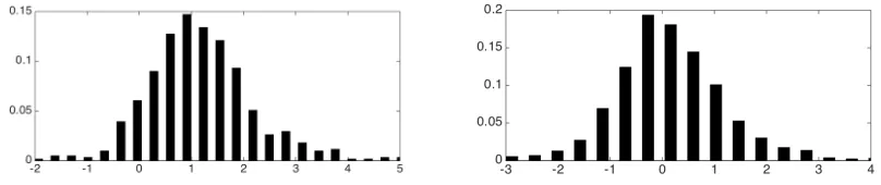
computers (κ0) relatively more than non-computer equipment (κ) within occupations (ω),
the left panel of Figure2plots the histogram of
logπt λ 0
,κ0,ω πt λ0,κ,ω
−logπt λ,κ 0
,ω πt λ,κ,ω
across all five years, thirty occupations, and six gender-age groups described above. Fig-ure 2 shows that college educated workers are relatively more likely to use computers within occupations compared to high school educated workers; hence, according to our model, college educated workers have a comparative advantage using computers within occupations relative to high school educated workers. A similar conclusion holds com-paring across other education groups: more educated workers always have a comparative advantage using computers.
Figure 2: Computer relative to non-computer usage for college degree relative to high school degree workers (female relative to male workers) in the left (right) panel
The right panel of Figure2plots a similar histogram, where λ0 and λnow denote
4.2
Measuring shocks
Here we describe our baseline procedure to measure the four shocks into which we de-compose changes in relative average wages: labor composition, ˆL(λ)/ ˆL(λ1), equipment
productivity (to the power θ), ˆq(κ)θ/ ˆq(κ1)θ, occupation shifters, ˆa(ω)/ ˆa(ω1), and labor
productivity, ˆT(λ)/ ˆT(λ1). We measure changes in labor composition directly from the
MORG CPS. We measure changes in equipment productivity using data only on changes in disaggregated factor allocations over time, ˆπ(λ,κ,ω). We measure changes in
occupa-tion shifters using data on changes in disaggregated factor allocaoccupa-tions and labor income shares across occupations as well as model parameters. Finally, we measure changes in labor productivity as a residual to match observed changes in relative wages. We pro-vide details on the baseline procedure described here in Appendix C.1 and alternative procedures in AppendicesC.2andC.3. All these procedures yield very similar results.
First, consider the measurement of changes in equipment productivity to the powerθ.
Equation (12) implies
ˆ
q(κ)θ
ˆ
q(κ1)θ
= πˆ(λ,κ,ω)
ˆ
π(λ,κ1,ω) (14)
for any(λ,ω)pair. Hence, if computer productivity rises relative to other equipment
be-tweent0andt1, then the share ofλhours spent working with computers relative to other
equipment in occupation ω will increase. It is important to condition on (λ,ω) pairs
when identifying changes in equipment productivity because unconditional growth over time in computer usage, shown in Table1, may also reflect growth in the supply of labor groups who have a comparative advantage using computers and/or changes in occupa-tion shifters that are biased towards occupaoccupa-tions in which computers have a comparative advantage. We combine these(λ,ω) pair-specific measures to obtain a unique measure
of changes in equipment productivity to the powerθ, ˆq(κ)θ/ ˆq(κ1)θ, as described in
Ap-pendixC.1.
Second, consider the measurement of changes in occupation shifters. Equation (13) implies
ˆ
a(ω)
ˆ
a(ω1)
= ζˆ(ω)
ˆ
ζ(ω1)
ˆ
q(ω)
ˆ
q(ω1)
(1−α)(ρ−1)
. (15)
We construct the right-hand side of equation (15) in two steps as follows. First, equation (12) implies
ˆ
q(ω)θ
ˆ
q(ω1)θ
= πˆ(λ,κ,ω)
ˆ
π(λ,κ,ω1)
(16)
measure of changes in transformed occupation prices to the powerθ, ˆq(ω)θ/ ˆq(ω1)θ, as
de-scribed in AppendixC.1.23 Given values ofα,ρ, andθ, we recover(qˆ(ω)/ ˆq(ω1))(1−α)(ρ−1).
We describe how we estimate these three parameters below. Second, given values of ˆ
q(κ)θ/ ˆq(κ1)θ and ˆq(ω)θ/ ˆq(ω1)θ, we construct ˆζ(ω)/ ˆζ(ω1) using the right-hand side of
equation (13). Note that if ρ= 1, changes in occupation shifters depend only on changes
in the share of labor payments across occupations.
Finally, we measure changes in labor productivity as a residual to match changes in relative wages. Specifically, we rewrite equation (11) as
ˆ
w(λ)
ˆ
w(λ1)
= Tˆ(λ)
ˆ
T(λ1)
ˆ
s(λ)
ˆ
s(λ1)
1/θ
, (17)
where ˆs(λ)is a labor-group-specific weighted average of changes in equipment
produc-tivity and transformed occupation prices, both raised to the powerθ,
ˆ
s(λ) =
∑
κ,ω ˆ
q(ω)θ
ˆ
q(ω1)θ
ˆ
q(κ)θ
ˆ
q(κ1)θ
πt0(λ,κ,ω), (18)
which we can construct using observed allocations, changes in observed allocations, and equations (14) and (16). Given wage data and a value of θ, we recover ˆT(λ)/ ˆT(λ1).
Note that only our measures of changes in labor productivities are directly a function of the observed changes in relative wages that we aim to decompose: given parameters
α, ρ, and θ, observed changes in wages do not affect our measures of changes in labor
composition or equipment productivity to the powerθ, and they only affect our measures
of occupation shifters indirectly through their impact on ˆζ(ω)/ ˆζ(ω1).
4.3
Parameter estimates
The Cobb-Douglas parameter α, which matters for our results only when ρ is different
from one, determines payments to all equipment (computers and non-computer equip-ment) relative to the sum of payments to equipment and labor. We set α = 0.24,
con-sistent with estimates in Burstein et al. (2013). Burstein et al. (2013) disaggregate total capital payments (i.e the product of the capital stock and the rental rate) into structures and equipment using US data on the value of capital stocks and—since rental rates are not directly observable—setting the average rate of return over the period 1963-2000 of
23We use data on observed allocations to measure these changes in transformed occupation prices. In
holding each type of capital (its rental rate plus price appreciation less the depreciation rate) equal to the real interest rate.
As a reminder, the parameter θ determines the within-worker dispersion of
produc-tivity across occupation-equipment type pairs and the parameterρis the elasticity of
sub-stitution across occupations in the production of the final good. We estimate these two parameters jointly using a method of moments approach. In order to derive the relevant moment conditions, we rewrite equation (17) as
log ˆw(λ,t) =ςθ(t) + (1/θ)log ˆs(λ,t) +ιθ(λ,t), (19) where ˆs(λ,t)is defined in equation (18), ςθ(t) ≡ log ˆq(ω1,t)qˆ(κ1,t)is a time effect that is common across λ, and ιθ(λ,t) ≡ log ˆT(λ,t) captures unobserved changes in labor productivity.24 Similarly, equation (13) can be expressed as
log ˆζ(ω,t) = ςρ(t) + ((1−α) (1−ρ)/θ)log ˆ
q(ω,t)θ
ˆ
q(ω1,t)θ
+ιρ(ω,t). (20)
where ˆq(ω,t)θ/ ˆq(ω1,t)θis defined in equation (16),ςρ(t)is a time effect that is common acrossω andιρ(ω,t)≡log ˆa(ω,t)captures unobserved changes in occupation shifters.
Equations (19) and (20) may be used to jointly identify θ and ρ. According to our
model, however, the observed covariate in equation (19), log ˆs(λ,t), is predicted to be
correlated with its error term, ιθ(λ,t), and the observed covariate in equation (20) is predicted to be correlated with its error term, ιρ(ω,t). To address the endogeneity of these covariates, we construct instruments using different averages of observed changes in equipment productivity to the powerθ, ˆq(κ,t)θ/ ˆq(κ1,t)θ. Specifically, we instrument
the covariate log ˆs(λ,t)using a labor-group-specific average,
log
∑
κˆ
q(κ,t)θ
ˆ
q(κ1,t)θ
∑
ωπ1984(λ,κ,ω),
and the covariate log ˆq(ω,t)θ/ ˆq(ω1,t)θusing an occupation-specific average
log
∑
κˆ
q(κ,t)θ
ˆ
q(κ1,t)θ
∑
λL1984(λ)π1984(λ,κ,ω)
∑λ0,κ0 L1984(λ 0)
π1984(λ0,κ0,ω)
.
We use these two instruments and equations (19) and (20) to build moment conditions that identify the parameter vector (θ,ρ).25
24For the purposes of this section, for any variablex, we use ˆx(t) to denote the relative change in a
variablexbetween any two periodstandt0 >t.
25Additional details on these moment conditions are provided in AppendixD. This appendix also
Our estimates exploit data on four time periods: 1984-1989, 1989-1993, 1993-1997, and 1997-2003. We report the point estimates and standard errors in the top row of Table 2. The resulting estimate of θ is 1.78 with a standard error of 0.29; the estimate of ρis also
1.78 but with a slightly larger standard error of 0.35.
In reviewing Krusell et al. (2000), Acemoglu (2002) raises a concern that may affect the estimates of θ and ρ computed using equations (19) and (20) as estimating
equa-tions. Specifically, they point out that the presence of common trends in unobserved labor-group-specific productivity, explanatory variables, and instruments may bias the estimates of wage elasticities. In order to address this concern, we followKatz and Mur-phy (1992) and Acemoglu (2002) and additionally control for a λ-specific time trend in
equation (19). In addition, we also control for an occupation-specific time trend in equa-tion (20). The MM estimates ofθandρthat result from adding as controls a
labor-group-specific time trend in equation (19) and an occupation-specific time trend in equation (20) are, respectively 1.13, with a standard error of 0.32, and 2, with a standard error of 0.71, as displayed in row 2 of Table2.26
Parameter Time Trend? Estimate (SE)
(θ,ρ) NO (1.78, 1.78) (0.29, 0.35)
(θ,ρ) YES (1.13, 2.00) (0.32, 0.71)
Table 2: Parameter estimates based on joint estimation
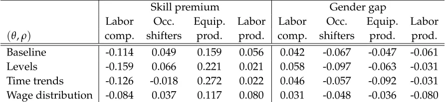
When computing the main results of our analysis, we verify in Appendix E.1the ro-bustness of our conclusions to the different estimates ofθ and ρ reported in this section
and in AppendixD.
4.4
Results
In this section we summarize the results of our decomposition of observed changes in relative wages in the US between 1984 and 2003 into the contributions of changes in la-bor composition, occupation shifters, equipment productivity, and lala-bor productivity. We construct various measures of changes in between-group inequality, each of them
aggre-and expected to be correlated with the corresponding endogenous variables.
26In AppendixDwe provide estimates ofθ andρ that rely on alternative identification assumptions.
First, we report MM estimates that use versions of both equation (19) and equation (20) in levels instead of time differences; the resulting estimates areθ=1.57, with a standard error of 0.14, andρ =3.27, with a
standard error of 1.34. Second, we followLagakos and Waugh(2013) andHsieh et al.(2016) and identifyθ
from moments of the unconditional distribution of observed wages within each labor groupλ; the resulting
estimate ofθis equal to 2.62. Finally, we also estimateθandρwithout instruments and show that the bias
gating wage changes across our thirty labor groups in different ways (e.g., the skill pre-mium). As is standard, when doing so, both in the model and in the data, we construct
composition-adjustedwage changes; that is, for each aggregated measure we report, we av-erage wage changes across the corresponding labor groups using constant weights over time, as described in detail in AppendixB. For each measure of inequality, we report its cumulative log change between 1984 and 2003, calculated as the sum of the log change over all sub-periods in our data.27 We also report the log change over each sub-period in our data.
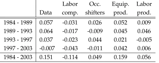
Skill premium. The first column in Table 3 reports the change observed in the data,
which is also the change predicted by our model when all shocks—in labor composition, occupation shifters, equipment productivity, and labor productivity—are simultaneously considered. The skill premium increased by 15.1 log points between 1984 and 2003, with the largest increases occurring between 1984 and 1993. The subsequent four columns summarize the counterfactual change in the skill premium predicted by the model if only one of the four shocks is considered (i.e. holding the other exogenous parameters at their
t0level).
Labor Occ. Equip. Labor Data comp. shifters prod. prod. 1984 - 1989 0.057 -0.031 0.026 0.052 0.009 1989 - 1993 0.064 -0.017 -0.009 0.045 0.046 1993 - 1997 0.037 -0.023 0.044 0.021 -0.005 1997 - 2003 -0.007 -0.043 -0.011 0.042 0.006 1984 - 2003 0.151 -0.114 0.049 0.159 0.056
Table 3: Decomposing changes in the log skill premium (the wage of workers with a college degree relative to those without)
Changes in labor composition decrease the skill premium in each sub-period. Specifi-cally, the increase in hours worked by those with college degrees relative to those without of 47.4 log points between 1984 and 2003 decreases the skill premium by 11.4 log points. Changes in relative demand across labor groups must, therefore, compensate for the im-pact of changes in labor composition in order to generate the observed rise of the skill premium in the data.
Changes in equipment productivity, i.e. computerization, account for roughly 60% of the sum of the demand-side forces pushing the skill premium upwards: 0.60 '0.159 / (0.049 + 0.159 + 0.056). Furthermore, changes in equipment productivity are particularly
27We obtain very similar results if we directly compute changes in wages between 1984 and 2003 instead
important in generating increases in the skill premium in those sub-periods in which the skill premium rose most dramatically: 1984-1989 and 1989-1993. These are also precisely the years in which the overall share of workers using computers rose most rapidly; see Table1. The intuition for why our model predicts that computerization had a large impact on the skill premium is the following. The procedure described in Section4.2to measure changes in computer productivity implies large growth in this variable.28 This growth raises the skill premium for two reasons, as described in detail in Section3.4. First, edu-cated workers have a direct comparative advantage using computers within occupations, as shown in Figure 2. Second, educated workers have a comparative advantage in oc-cupations in which computers have a comparative advantage and, given our estimate of
ρ, this implies that computerization raises the wages of labor groups disproportionately
employed in computer-intensive occupations.
Changes in occupation shifters account for roughly 19% of the sum of the forces push-ing the skill premium upwards. Skill-intensive occupations grew disproportionately in our sample period, as documented in Figure 1 and in Table9 in Appendix B. If ρ = 1,
then this growth would be attributed fully to occupation shifters and occupations shifters would have accounted for a larger share of the growth of the skill premium as shown in our sensitivity analysis in Appendix E.1. However, because ρ 6= 1, other shocks also
affect income shares across occupations. In AppendixH.1we document the importance of each shock for the growth of occupations with different characteristics (using O*NET constructed task measures).
Finally, labor productivity, which we estimate as a residual to match observed changes in relative wages, accounts for roughly 21% of the sum of the effects of all three demand-side mechanisms.
In AppendixE.2 we demonstrate the importance of accounting for all three forms of comparative advantage by performing similar exercises in versions of our model that omit some of them.
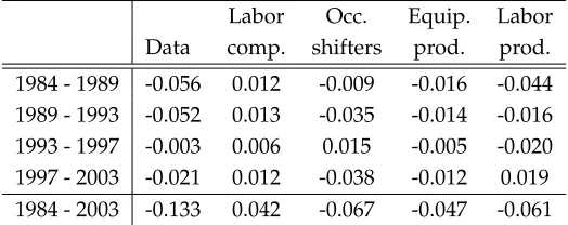
Gender gap. The average wage of men relative to women, the gender gap, declined
by 13.3 log points between 1984 and 2003. Table 4 decomposes changes in the gender
2